


Introduction
Floods are the most common natural disasters in the world. From 2000 to 2019, they accounted for 43% of 7,348 recorded disasters around the world affecting 4.3 billion people (CRED and UNDRR, 2020). In the U.S., floods were responsible for $200 billion in cumulative damages from 1988 to 2017 (Davenport et al., Reference Davenport, Burke and Diffenbaugh2021). Floods also represent a unique policy challenge. Private insurers are reluctant to write flood insurance policies due to information asymmetries, correlated risks, and large, lumpy losses. In addition, there exists no private industry aimed at post-disaster clean-up and remediation. Thus, it falls to governments to establish and regulate flood insurance markets and oversee post-disaster relief and recovery following flood events (Moss, Reference Moss1999; Kousky, Reference Kousky2018).
In the U.S., flood insurance policies are predominantly written and backed by the federal government via the National Flood Insurance Program (NFIP). Footnote 1 The NFIP, which was created in 1968 in response to a lack of private flood insurance, is housed in Federal Emergency Management Agency (FEMA). The program is responsible for mapping flood risk, establishing flood zone boundaries and nationwide flood insurance rates, collecting premiums, and paying claims. Footnote 2 The actual program works through a system of communities with each community voluntarily choosing to join in exchange for receiving access to the federal flood insurance market. Admission is based on, among other things, the adoption of baseline floodplain management designed to limit future damages from floods. The early years of the NFIP saw limited participation and insurance take-up. However, in 1973 Congress passed the Flood Disaster Protection Act, which tied flood insurance directly to homeownership. Footnote 3 While the act led to a steady increase in participation, it failed to address the remaining issues of solvency and affordability; it also provided limited incentives for communities to go beyond baseline floodplain management. Footnote 4
In 1990, FEMA introduced the Community Rating System (CRS) to increase support for the NFIP. CRS is an incentive program focused on reducing and avoiding flood damage to insurable properties, strengthening and supporting the insurance aspects of the NFIP, including the expansion of the policy base, and fostering comprehensive floodplain management (FEMA, 2017b). To achieve its goals, CRS provides premium discounts in exchange for flood management activities (investments) that go beyond baseline NFIP requirements. Communities earn points from their investments, which range from information campaigns and map updates to land preservation and home removals with additional points leading to additional discounts. Because the program is designed to be revenue neutral, non-CRS communities cross-subsidize CRS communities. Specifically, as CRS communities gain points and improve their ranking their discounts are offset by increased premiums in non-CRS communities (Kousky, Reference Kousky2018). Given this structure, it is important to understand the distributional impacts of any gains and losses from how the CRS changes NFIP premiums. Specifically, it is instructive to know: (1) what do the distribution of gains and losses look like and (2) how are the gains and losses correlated with community socioeconomic factors and measures of flood risk. Footnote 5
We first look at what factors explain premium differences induced by CRS. We define gains and losses at the policy level based on whether a household’s flood insurance premium is lower or higher than what it would be without CRS. We use NFIP policy data from 2009 through 2019 and create counterfactual policies representing a world without CRS. Footnote 6 Specifically, we use the CRS-adjusted insurance premiums from the raw FEMA data, information of the CRS classes of all NFIP communities and their discounts contained in that data, and information on how CRS cross-subsidies are structured to recover unadjusted premiums for each household, i.e., undiscounted premiums as they would be without the CRS program in place – our counterfactual premiums. Footnote 7 To understand who is impacted, we take the difference between the actual premiums in the data and our counterfactual premiums and regress the difference on variables representing the characteristics of the policyholders in each NFIP community. We are particularly interested in how income, education, race, population, and flood risk correlate with the transfers created by the CRS program.
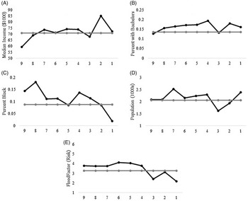
To establish a baseline set of hypotheses (expectations) related to CRS participation, cross-subsidization, and the socioeconomics of the underlying communities, we follow recent work examining the relationship between demographics and community rank within the program; we also look at the relationship between the underlying flood risk in a community and its CRS rank (Gourevitch and Pinter, Reference Gourevitch and Pinter2023). Figure 1, panels A.–D., shows the mean value for median income, the percent of the adult population with a four-year degree, percent black, and total population by CRS class across all communities and years in our data. In panel E., we show the mean value for flood risk, based on First Street Foundation’s risk designation, for each community and year. All values are based on census block group data merged with the NFIP community boundaries. The black line shows the mean values for each variable by CRS class, and the gray line is the mean value for non-CRS communities. Based on these figures and the fact that most CRS communities are concentrated in classes 5–8, we expect income and population to play a minimal role in explaining CRS cross-subsidization and communities with higher shares of people with bachelor’s degree and those with higher shares of black families to gain the most from the cross-subsidies. We also note that CRS communities with higher discounts have a higher level of flood risk compared to those with lower discounts and those outside the CRS program.
Mean demographics by CRS class. Note: The figure shows mean demographics (A.–D.) and mean flood risk (E.) across NFIP communities by CRS class. Demographics are based on census block group data spatially merged with the NFIP community boundaries. Flood risk is based on First Street Foundation’s Flood Risk Factor, a variable that ranges from low risk (1) to high risk (10), which is aggregated up to the census block group. The black line is the mean value for each CRS class. The gray line is the mean value for all non-CRS communities.

In addition to examining the impact of location characteristics on cross-subsidization, we also look at the interaction of the CRS program with FEMA’s Hazard Mitigation Assistance (HMA) grant program. NFIP communities enter CRS and gain points by making investments in floodplain management. There are costs associated with these activities, but the source of the funds used to cover these costs is not always clear. One source is local tax (income and property) revenue, and previous research has shown that local financial capacity is a factor impacting local flood hazard mitigation (Landry and Li, Reference Landry and Li2012). Another source is money from federal cost-share programs, such as the HMA program, which provide financial assistance to states and municipalities in reducing their risks from natural hazards and their reliance on federal disaster funds (FEMA, 2015). Here, we are interested in how HMA grants are correlated with CRS participation. If communities use HMA funds to cover investment costs that translate into CRS discounts, then it has clear implications for redistribution – the costs are being funded by the taxpayer, while the community gains the benefits from reduced insurance premiums.
Our results provide a number of important insights. We find that the CRS program does result in premium redistribution, but the most significant impact is only related to raw policy counts. We find that while 68% of NFIP policies are written in CRS communities, after accounting for the structure of CRS over 65% of policyholders cross-subsidize the remaining 35%, i.e., 65% of policyholders see their premiums increase, while the remaining minority see them decline. In terms of the actual monetary gains and losses, the numbers are modest for most policyholders. Looking at the distribution of annual gains and losses during our study period, we find that 90% of the gains/losses fall in the range of −$146 to $105 and 95% fall in the range of −$214 to $156. Using real median household income across all NFIP communities, these values imply that 90% of households gain or lose no more than 0.2% of their income and 95% gain or lose no more than 0.3%. The relatively small distributional effect is likely because of the small percentage of policies with high CRS discounts, i.e., less than 1% of policies have discounts greater 25%, since it is primarily the high discount policies that generate the largest premium transfers. Thus, the economic welfare implications of the program appear muted, at least based on the fundamentals in place during our study period.
Looking at correlations between premium changes and local characteristics, we find that communities with higher education and more people, those with older populations, and those in urban areas see premiums decline, while rural places and those with higher incomes see their premiums increase. More importantly, we find that places with more flood risk see their premiums decline and that flood risk is the single biggest predictor of premium changes. Specifically, the coefficient on our flood risk variable is twice as large, in standardized form, as any other variable in the model. While this suggests that CRS is making it cheaper to live in riskier locations, i.e., the CRS program provides a net incentive to reside in risky locations, we do not think it is likely to impact relative household sorting. Because the gains and losses in premium dollars represent such a small share of household income, they are unlikely to impact where households choose to live.
We also find a positive relationship between HMA grants and CRS points and discounts with the receipt of a HMA grant increasing CRS points by 68 and increasing discounts by 0.55%. We find a particularly strong result for points gained in investment activities related to property acquisition and relocation and drainage system management, all of which are expensive investments. This suggests that HMA grant dollars may have a particularly large impact in helping communities make up funding deficits in these areas; it also suggests another path for redistribution since most of these dollars come from federal tax revenue.
Our paper contributes to the growing literature evaluating the CRS program. A number of papers have looked at drivers of CRS participation and its impact on NFIP participation (Frimpong et al., Reference Frimpong, Petrolia, Harri and Cartwright2020; Li and Landry, Reference Li and Landry2018; Sadiq and Noonan, Reference Sadiq and Noonan2015; Landry and Li, Reference Landry and Li2012). Li and Landry (Reference Li and Landry2018) find a correlation between past and current CRS points, and they find that places with higher government revenues and income, higher population density, and older households all have greater amounts of mitigation. They, along with Sadiq and Noonan (Reference Sadiq and Noonan2015) and Landry and Li (Reference Landry and Li2012), also find that past flood experience and local flood risk factors drive CRS participation and CRS discounts. In our model, we find that flood risk is positively correlated with a decline in premiums, which follows from communities in riskier areas joining and improving their CRS ranking.
Other papers have examined the relationship between CRS participation and damages (Frimpong et al., Reference Frimpong, Petrolia, Harri and Cartwright2020; Highfield and Brody, Reference Highfield and Brody2017; Brody et al., Reference Brody, Zahran, Maghelal, Grover and Highfield2007). Brody et al. (Reference Brody, Zahran, Maghelal, Grover and Highfield2007) found that nonstructural methods, such as CRS, while providing low-cost means of reducing property damages, may indirectly encourage development in hazardous areas. Highfield and Brody (Reference Highfield and Brody2017) found that the CRS program has led to a reduction in insured flood losses and an overall reduction in claims. More recently, Frimpong et al. (Reference Frimpong, Petrolia, Harri and Cartwright2020) found that CRS participation is associated with lower flood damage claims, but only in communities that have achieved a CRS class 5 status or lower, a status level that represents only around 18% of all NFIP policies.
In research closest to ours, Noonan and Sadiq (Reference Noonan and Sadiq2018) look at the effect of CRS on poverty and income inequality, and Noonan and Liu (Reference Noonan and Liu2019) look at the effect of CRS participation and flood risk on local patterns of population change. Using panel data at the tract level from 1970 to 2010, Noonan and Sadiq (Reference Noonan and Sadiq2018) find that median incomes are lower and poverty rates are higher in CRS communities. We find similar results for income – higher-income communities cross-subsidize lower-income communities. However, we find that places with higher education are cross-subsidized by those with lower education, which works in the opposite direction to the extent that education is positively correlated with income. Noonan and Liu (Reference Noonan and Liu2019), again using tract-level data from 1970 to 2010, find that CRS, and flood risk more broadly, leads to population turnover. However, they do not find any evidence that CRS is pushing populations toward or away from low- or high-risk areas. Their hypothesis is that CRS-induced premium changes have not been large enough to affect household sorting. We find support for this claim given the relatively small size of gains and losses in our data. What distinguishes our research from the existing literature on the CRS is as follows: (1) we find a way to calculate counterfactual premium for each policy, which allows us to compare the premium change in a world with and without the CRS program and (2) we use policy-level data to understand the distributional impact at the household level. We also relate these policy-level changes to flood risk and connect it to other federal policies.
The remainder of the paper is structured as follows. Section “Data and policy background” introduces the data collected for the paper and the construction of the final data sets used in our models as well as an overview of the CRS program. Section “Empirical models” introduces our empirical models and provides a detailed discussion of how we created our counterfactual insurance premiums. Section “Results” presents our results, and Section “Conclusion” concludes.
Data and policy background
Data sets
The data in this paper come from several sources. First, we submitted a Freedom of Information Act (FOIA) request to FEMA to obtain historical data on flood insurance policies, policy claims, and the CRS program. The policy data included information on each policy’s census block group, CRS class and discount, flood zone, annual premium, house type, and effective policy date. The CRS data included information about all communities that participated in CRS dating back to 1998, their CRS class, total points earned, and details about their credited activities. The claims data recorded the time and amount of all claims of NFIP policyholders.
Second, we downloaded a geospatial database of all NFIP communities – the National Flood Hazard Layer (NFHL) – and spatially linked it to our policy, claims, and CRS data as well as to census block group data on the socioeconomic characteristics of the NFIP communities. These data showed the exact location and boundaries of each NFIP community and the SFHA region within each community.
Third, we downloaded HMA grant and historical disaster declaration data from the OpenFEMA website. The HMA data provided information about funded projects including each project’s location and type, total funding, and the federal cost-share amount. The disaster data gave the date and time for each presidential disaster declaration occurring during our study period.
Fourth, we downloaded demographic and economic data at the census block group level from IPUMS (Manson et al., Reference Manson, Schroeder, Riper, Tracy and Ruggles2021). The IPUMS data are based on the American Community Survey (ACS) and include information on population, race, median household income, education, age, household composition, median home value, urban status, employment, and health insurance.
And finally, we obtained a property-level measure of flood risk from the First Street Foundation (First Street Foundation, 2021). First Street uses a first-of-its-kind methodology to analyze past disaster outcomes, current flood hazards, future climate scenarios, and local adaptation efforts to provide individual properties across the U.S. with measures of flood risk. At a high level, their model incorporates the four major contributors to flooding: tidal, rainfall, riverine, and storm surge. By taking property-level data, overlaying building footprints, and applying the flood hazard layers they calculate the maximum flood depth for each building or lot. Footnote 8 Flood risk is defined as a combination of cumulative risk over 30 years and flood depth. Their measure provides an integer value to each property ranging from 1 (lowest risk) to 10 (highest risk).
Our decision to use First Street data as our measure of flood risk stems from the fact that it is the most up-to-date (accurate) and publicly available housing-level measure of flood risk. This does not imply, however, that First Street’s measure is the most salient to the average household. In most cases, the most salient flood risk information for households likely comes from the NFIP’s Digital Flood Elevation Insurance Maps (DFIRMs). These maps, however, do not accurately reflect all flood risk as there are often long lags between map updates and changes in risk; also, FEMA maps have not historically reflected future climate change projections. In this paper, we are most interested in how the distribution of CRS discounts correlates with true measures of flood risk regardless of whether households perceive those actual risks or not. Thus, we choose to use the First Street data as it comes closest to achieving this goal. In the results section we provide results from a robustness model where we swap out the First Street risk measure for a measure based on flood risk defined by the NFIP’s DFIRMs.
We combine all of our data sets to answer our research questions related to the distributional impact of the CRS program. Section “Community rating system” provides a brief overview of the CRS program and our CRS data. Then, in Section “Cross-subsidization and insurance premiums” we describe the construction of the data used in analyzing the impact of cross-subsidization on flood insurance premiums, and in Section “CRS participation and HMA grants,” we describe the construction of the data used our analysis of the impact of HMA grants on CRS participation.
Community rating system
The community rating system (CRS) was introduced by FEMA in 1990 as a supplement to the NFIP program. CRS is a voluntary incentive program that allows NFIP communities Footnote 9 who adopt floodplain management activities that exceed the minimum requirements needed for NFIP membership to receive points that translate into discounts on flood insurance premiums as they improve their CRS class. There are 19 different types of activities in the CRS program categorized into four groups: Public Information Activities, Mapping and Regulations, Flood Damage Reduction Activities, and Warning and Response. Each activity has a specific point total associated with it, and communities accumulate points by partial or fully executing the activities in each category. As communities accumulate points, they move up in their class rank with 10 being the lowest and 1 being the highest. With each improvement in class, the reduction in flood insurance premiums goes up with discounts varying between SFHA and non-SFHA policies.
Table 1 provides a full list of CRS activities, their categories, the maximum number of points a community can earn for each activity, and the average number earned across the entire CRS program. Table 2 shows the CRS points needed for each CRS class and the associated discounts by flood zone type. The values in the first four columns are taken directly from FEMA’s website. Footnote 10 The last two columns are created from our NFIP policy data. In column 5 (Share of CRS Policies), we show the share of policies from CRS communities that fall within each community class. Most of the policies are written in communities with a class rank of 5-8. In column 6 (Share of All Policies), we show policies from each community class as a share of all policies in the NFIP program. Summing these up shows that approximately 66.7% of all NFIP policies are written in CRS communities.
Maximum and average CRS points earned by activity

Note: This table reports data from FEMA on the maximum number of points available for each activity in the CRS program and the average number of points earned by participating communities within the program as of 2017 (FEMA, 2017b).
Overview of the CRS program

Note: This table presents an overiew of FEMA’s CRS program. Columns 1-4 are taken directly from FEMA’s website for the program and show the program classes (column 1), the point ranges that can be earned (column 2), and the discounts for those classes and ranges for properties inside (column 3) and outside (column 4) of the SFHA. Data from these columns come from (FEMA, 2017b). Columns 5 and 6 show the distribution of policies written in CRS communities from the policy data used in this paper. Column (5) shows the distribution shares across communities just for policies written in CRS communities, and column (6) shows it as a share of all policies in the NFIP program.
Generally, as one moves from 300-level activities to 600-level activities the costs associated with the activity rise as well. For example, acquiring and/or relocating buildings (520) is a much bigger task than simply providing flood risk information (320–340). This would suggest that most communities who join CRS remain in higher classes with smaller discounts, which is exactly what we find. Based on our data, the average class rank across the CRS program is 7.4, which translates to a roughly 12.5% discount on insurance premiums; it also indicates that most communities do not invest a lot of resources in CRS activities. Footnote 11
Data construction
Cross-subsidization and insurance premiums
Our model on cross-subsidization is estimated at the policy and year level from 2009 through 2019. While our FOIA request resulted in policy data as far back as 1978, FEMA’s website states that policy data prior to 2009 is unreliable as FEMA did not retain complete policy records prior to that year. So, we limit our policy sample to the years 2009–2019 since our FOIA request resulted in only partial coverage for 2020.
Since all models are estimated based on calendar years, we use each policy’s effective date, which is the date the policy went into force, to assign a policy to a calendar year. We also limit our analysis to single-family houses and those with a single policy on the property. This is not particularly restrictive since the majority of policies – 84.8% in the full data – were written for single-family residences. It also limits the inclusion of commercial policies, which we want to exclude. And finally, we drop all observations with negative premiums and those with premiums above and below the top and bottom 1% in the data (Bradt et al., Reference Bradt, Kousky and Wing2021). Our final data set contains roughly 38.25 million policy-by-year observations.
Using our cleaned policy data, we merge in socioeconomic and flood risk data at the block group level. The socioeconomic data are based on five-year ACS data samples. For each year in the policy data, we use the five-year ACS data estimates that straddle that year. Thus, we have updated estimates of all sociodemographic variables for each year in the policy data.
To obtain our community-level measure of flood risk, we calculate the average of First Street’s house-level Flood Factor for houses in each census block group and attach the value to policies based on their block group. We also calculate a similar measure of flood risk at the block group level using the FEMA’s maps for the SFHA boundaries for A and V zones.
Table 3 reports summary statistics for the policy data used in our premium difference model (Section “The distributional effect of CRS”). The first variable in the table, DisPolicyPremium, provides summary statistics for the premiums paid by policyholders as they show up in the raw FEMA data. The values reflect the premiums paid by all households across the NFIP program after CRS discounts and cross-subsidies have been included. Thus, while the values for the raw premium values are all positive, they are higher or lower than they would be without the CRS program depending on whether a household is outside or inside a CRS community.
Summary statistics for data used in the CRS model

Note: The sample comprises 38,054,192 policy records from 2009 through 2019. DisPolicyPremium is the household insurance premium observed in the raw FEMA data, which includes the CRS discount as part of the premium paid. PremDiff, the outcome variable in our CRS model (equation 1), is constructed by taking the difference between the DisPolicyPremium variable and a counterfactual premium value for each household constructed by removing all CRS discounts. InCRS is a binary variable for whether a policy was in a CRS community. AZone, VZone, and SFHA are the % of land area in each census block group classified as A zone, V zone, or SFHA, respectively. FloodFactor is an indicator of comprehensive flood risk taken from First Street’s house-level flood risk data indicator, FloodFactor. All of the remaining variables are based on block group-level averages for socioeconomic variables using American Community Survey data attached to individual policies based on their census block group.
The second variable in the table, PremDiff, is the outcome variable in our CRS model (equation 1). This variable takes on positive and negative values because we take, for each policyholder, the value for the DisPolicyPremium in the raw data and subtract from it a counterfactual value produced by “undoing” CRS discounting built into each household’s insurance premium. Thus, some households, in a world without CRS, see their premiums rise and others see them fall. We provide a full explanation for the construction of this variable in Section “The distributional effect of CRS”; a full distribution of this variable is shown in Figure 2.
Statistics for distribution of premium differences. Note: The figure shows statistics describing the distribution of PremDiff outcome variable in our CRS model (equation 1). The premium differences are produced by subtracting counterfactual premiums, i.e., those produced after removing CRS discounts, from the CRS-adjusted premiums that show up in the raw FEMA data. The values take on positive and negative values because, after removing CRS subsidies, some households would see their premiums increase and others see them decrease.

The third variable in the table, InCRS, is an indicator of the policy’s CRS status. It is an indicator of whether the policy was written in a CRS community. Once again, the mean value of 67.5% reflects the fact that a relatively large number of policies are written in CRS communities. While only 10% of NFIP communities are in CRS, around 70% of NFIP policies are written in CRS communities (FEMA, 2017a).
The remaining variables in Table 3 are summary statistics for the flood risk variables – the second group of variables – and the sociodemographic variables – the third group of variables – that are used in our CRS empirical model presented in the next section.
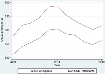
Figures A3 and A4 in the appendix provide more context to our policy data. Figure A3 shows the average of the DisPolicyPremium over time. As expected, the average premium in CRS communities is $52–$83 lower than in non-CRS communities. The figure also shows a general increase in premiums over time, which is likely driven by premium increases in response to FEMA’s mounting debt within the NFIP program. Figure A4 shows the number of policies in force by CRS status over time. This figure shows a clear downward trend for both types of communities with a steeper decline in non-CRS communities.
CRS participation and HMA GRANTS
Our model of the relationship between HMA grants and CRS status is estimated at the community and year level. We estimate the model at this level for two reasons: (1) it is the community that joins NFIP and CRS and makes decisions on flood risk investments and (2) this is the smallest spatial scale at which we can attach HMA grant and project information. To produce our baseline CRS-HMA panel data set, we use the population of NFIP communities from the NFHL geodatabase and merge in CRS status and rank by year for each community from 2009 through 2019 using the CRS data from FEMA. Our final data set consists of 6,325 CRS Community-Year observations. Note that our panel data set includes only CRS communities, so it is unbalanced as not all communities are in CRS in all years.
Using these baseline data, we merge in the HMA grant data using NFIP ID numbers for each project in each year. Footnote 12 It is not exactly clear from the HMA data set when a community receives their funding after their application is approved as there are three variables related to approval: initial approval, approval, and close date. So, we use approval date to determine the year when a community receives their funds.
Finally, we merge in data on demographics and other control variables. While our CRS-HMA data are at the community level, our other data are at the block group or county level. To identify the overlap between these spatial units and the CRS communities, we intersect their shapefiles and the shapefile from the NFHL geodatabase using ArcGIS software and calculate geographic weights indicating the percentage of each spatial united located in a CRS community. Figure A5 in the appendix provides an example of how we calculate the spatial weights and aggregate to them to the community level for block groups. After creating the spatial weights, we merge in data on demographics, policy claims, and presidential disasters. We document disaster declarations at the county-year level and merge by county code. For claims, we generate total claims paid in each block group in each year by adding the amount paid on building and contents. For demographics, we use IPUMS-ACS data and merge by block group and year.
Summary statistics for the final HMA-CRS data set are shown in Table 4. The first two variables are points earned and discounts obtained for each CRS community and year. These represent the outcome variables in our empirical model. The next set are HMA variables, which are our variables of interest. The first two are indicators for whether a community received an HMA grant, and the next three represent dollar amounts received for HMA projects. HMAAmountFed is the amount received in federal cost-share, and HMAProjectTotal is the total amount of the project. The remaining variable represents community-level sociodemographic variables – group three – and variables in flood risk, flood claims, and whether the community had a presidential disaster – the fourth group.
Summary statistics for data used in the HMA model

Note: This table describes the sample for the analysis of the impact of HMA grants on CRS participation. It comprises 6,325 CRS community-years observations from 2009-2019. HasHMA is a dummy variable for whether a community receives HMA grant in a given year; HMAAmountFed is the total amount of federal cost-share dollars received in millions of dollars; and HMAProjectTotal is the total cost of the project in millions of dollars. SFHA is % of land area in community classified as SFHA.
Empirical models
The distributional effect of CRS
The CRS program covers the costs, in terms of lost revenue, from the discounts on flood insurance premiums in CRS communities by increasing premiums on policyholders in non-CRS communities. These lower rates introduce explicit cross-subsidies into the program. While this process was intended to promote better flood risk management, it raises important questions about who wins and losses and the size of the gains and losses. Note that we are not trying to assess how commensurate the CRS discounts received by CRS participants are with their investments on CRS activities. We treat the costs of these investments as “sunk costs” and focus on how the subsidies are distributed across communities and how correlated they are with local community characteristics.
To analyze the distributional impacts of the CRS program’s cross-subsidization, we estimate the following empirical model:
 $$PremDif{f_{it}} = {\beta _i}{X_{it}} + {\varepsilon _{it}}.$$
The outcome variable, $PremDif{f_{it}}$
, is the difference between the premium paid by policyholder
$PremDif{f_{it}}$
, is the difference between the premium paid by policyholder $i$
in year
$i$
in year $t$
in a state of the world with the CRS in place versus the premium paid in a world without it. The value will be positive for households in non-CRS communities or for those in higher-class communities since their premiums would be lower without CRS, and it will be negative for households in lower-class CRS communities. Thus, we define negative premium differences as “gains” and nonnegative differences as “losses.” We provide an explicit explanation of this process and our counterfactual policy premiums below.
$t$
in a state of the world with the CRS in place versus the premium paid in a world without it. The value will be positive for households in non-CRS communities or for those in higher-class communities since their premiums would be lower without CRS, and it will be negative for households in lower-class CRS communities. Thus, we define negative premium differences as “gains” and nonnegative differences as “losses.” We provide an explicit explanation of this process and our counterfactual policy premiums below.
The purpose of the model in equation 1 is to explore which factors drive premium differences, i.e., which socioeconomic factors are associated with gains and losses within the CRS program. To test this, we regress our outcome variable on various socioeconomic variables including household income and education, race, home values, and urban status as well as on variables describing community flood risk. Note that we don’t have data on household-level socioeconomic characteristics, so all the covariates in equation 1 are at census block group level and we assume that households within the same block group have similar characteristics. We estimate all models in standardized form, so the coefficients represent the average increase or decrease in yearly premiums for a standard deviation change in each explanatory variable.
The positive and negative values for the outcome variable in our CRS model are the result of losses and gains resulting from cross-subsidies in the CRS program. Thus, construction of the variable requires knowing premiums with and without CRS. Premiums inclusive of CRS discounts are observed in the actual policy data. We have to construct the counterfactual premiums by reversing the premium adjustment process developed by FEMA for CRS.
Undoing the FEMA adjustment process recovers the “actuarially fair” premiums determined by FEMA for the NFIP in a world without CRS. Footnote 13 The intuition for this process is as follows. First, FEMA calculates the premium for each policyholder with and without CRS and sums them up to determine the total revenue collected with and without CRS. Then, the discounts for policyholders in CRS communities are accounted for by adjusting the baseline premiums of all policyholders in the NFIP upwards so that total revenue in the program is enough to cover expected losses that will occur at properties that have a CRS discount (Horn and Webel, Reference Horn and Webel2021). These adjustments vary over time, but not across policies in a given year. Footnote 14 To provide intuition for this process, we develop a simple example. The results are shown in Table 5.
Example of counterfactual CRS policies

Note: This table presents a numerical example demonstrating how we construct our counterfactual premiums – those that would exist without CRS. The table shows hypothetical results for two flood insurance policies for two communities, one CRS and one Non-CRS. Column (1) shows the premiums we observe in the data, which include the CRS adjustments based on the CRS discounts in column (2). The discounts – 0.25 and 0.15 – are based on communities with ranks of Class 5 and Class 7, respectively.
The table shows four hypothetical flood insurance policies, two in CRS communities (lines 1 and 2) and two in non-CRS communities (lines 3 and 4). Column (1), Observed Premiums, shows the values we observe in the policy data received from FEMA – the premiums with the CRS adjustments built in. We have set all premiums to $500 for simplicity. Column (2) shows the CRS discounts associated with each policy. As expected, discounts are only positive for the two CRS communities. The discounts in this example are associated with a Class 5 ranking (0.25 discount) for the first policy and a Class 7 ranking (0.15 discount) for the second policy. In column (3), Premiums w/o CRS, we use the CRS discounts and the observed premiums to undo the discounting associated with CRS. We then sum up the total premium revenue in column (1) in the CRS world ($2,000) and the total in column (3) in the non-CRS world ($2,255) and take the ratio to produce the FEMA Adjustment Factor in column (4). Finally, we multiple this adjustment factor by the premiums in column (3) to recover what we call the Counterfactual Premiums in column (5). In actuality, these values represent baseline NFIP flood insurance premiums or those that would be paid if the CRS program did not exist. Taking the difference between columns (1) and (5) produces the Gain or Loss in column (6), which is the outcome variable in our CRS model in equation 1. As expected, the two CRS communities see a decrease, and the non-CRS communities see an increase. Column (7) shows the gains and losses in percentage terms.
Our premium prediction method is based on several assumptions: (1) the total revenue collected from premiums remains neutral, i.e., total revenue needed with and without CRS is the same; (2) after removing the CRS discount there is a uniform discount applied to all policies to keep revenue neutral; (3) the removal of CRS will not lead to a change in the total number of policies in place; and (4) the removal of CRS will not impact total damages. The first two assumptions are likely to have limited impact as our method of reverse engineering the CRS adjustments follows the FEMA method very closely. The last two assumptions are more consequential.
Previous research has shown a positive relationship between CRS participation and the number of policies in force (Frimpong et al., Reference Frimpong, Petrolia, Harri and Cartwright2020) as well as a negative relationship between CRS participation and flood damage claims, at least for communities with CRS Class 5 and above (Brody et al., Reference Brody, Zahran, Maghelal, Grover and Highfield2007; Highfield and Brody, Reference Highfield and Brody2017). To examine how our results are impacted by relaxing assumptions (3), we develop a simulation that assumes removing CRS will change the demand for flood insurance. We use the simulation to generate counterfactual data and use the simulated data to re-estimate equation 1
We begin by borrowing values for the price elasticity of demand for flood insurance from previous research. Landry and Jahan-Parvar (Reference Landry and Jahan-Parvar2011) provide price elasticity estimates for flood insurance in coastal regions that range from −1.55 for subsidized policies to −0.13 for unsubsidized policies. More recently, Bradt et al. (Reference Bradt, Kousky and Wing2021) estimated the price elasticity of demand to be −0.29 for policies outside of the SFHA and −0.33 for houses within the SFHA. Since our data includes houses in coastal areas as well as inland regions, we use the values from Bradt et al. (Reference Bradt, Kousky and Wing2021) for SFHA and non-SFHA houses to predict the changes in insurance purchases following CRS-induced price changes.
For our simulation, we first bin all policy holders into groups each year based on their CRS discounts. Then, within each group we use the average premium difference, constructed using the method described above, and the elasticity values from the literature to predict the flood insurance demand responses for policies inside and outside of the SFHA. Finally, we randomly sample, with replacement, policyholders within each CRS group based on the predictions of demand for SFHA and non-SFHA households. This quasi-bootstrap simulation allows us to randomize the demand response to CRS-induced price changes based on empirical elasticity values.
Another potential concern related to assumption (3) is that participation in the CRS may impact the composition of policies and thus the future premium that’s based on local flood risk. We argue that this may not be the case for the following reasons. The discount the CRS program provides is a percentage reduction of the base premium which is determined mainly by flood zone type and adjusted by other factors (Kousky, Reference Kousky2018). The base premium for each flood zone is set nationally by FEMA. In other words, two properties with similar structural features located in an A zone in Texas or Georgia, in or out of the CRS program, have similar base premiums. In addition, although FEMA has been working on updating the Flood Insurance Rate Maps within the new FEMA Risk Rating 2.0 program, the insurance rates in our data do not vary by house based on local flood risk factors and are not actuarially fair (National Research Council, 2015).
To relax assumption (4), we borrow results from Frimpong et al. (Reference Frimpong, Petrolia, Harri and Cartwright2020) showing that damages fall by 5.8% in CRS communities of class 5 or lower relative non-CRS communities. For example, a CRS community with class 5 has a claim of $94.2, which is 5.8% reduction from $100. To reverse the damage reduction effect, we could get the claim without the CRS as $100 = 94.2/(1–0.58%). We calculate the increased claims for all CRS communities with CRS class 5 or better and then aggregate to annual flood damage increase. We then compare the increased annual claims to total revenue required for NFIP program after removing the CRS. The results show that after removing the CRS, the annual revenue required for the NFIP increases by 1% to 36% from 2009 to 2019 due to flood damage increase (2017 is an outlier because of several very costly hurricanes happened in that year).
The impact of HMA grants on CRS outcomes
In the previous section, we analyzed which factors explain gains and losses, in terms of insurance premium changes, that result from CRS. However, the decision to join CRS and allocate resources to CRS activities is made at the community level. In this section, we explore which factors drive communities to earn more CRS points and obtain better CRS discounts. We are particularly interested in the impact of HMA grants, which use a federal cost-share to help state and local communities make investments that reduce or eliminate risks from natural disasters. If some of the HMA funding goes to fund projects, which communities use to earn CRS credits, then the HMA program could accelerate the distributional impacts of CRS on NFIP policyholders. In other words, if receiving HMA grants increases CRS discounts, then the costs born by non-CRS communities may increase.
To explore this question, we estimate the following model:
 $${Y_{it}} = {\alpha _i} + {\beta _1}{\rm{HM}}{{\rm{A}}_{it}} + {\gamma _i}{X_{it}} + {\delta _t} + {\varepsilon _{it}}.$$
The outcome variable, ${Y_{it}}$
, is either total CRS points earned or the CRS discount for community
${Y_{it}}$
, is either total CRS points earned or the CRS discount for community $i$
in each year
$i$
in each year $t$
. Since premium discount across flood zones within a community could be different, here we calculate the community-level CRS discount as the ratio of aggregated discounted premium over aggregated total premium for a community. Our coefficient of interest,
$t$
. Since premium discount across flood zones within a community could be different, here we calculate the community-level CRS discount as the ratio of aggregated discounted premium over aggregated total premium for a community. Our coefficient of interest, ${\beta _1}$
, measures the marginal effect of receiving HMA grants. We use two measures of HMA grants in our models: an HMA grant indicator and a dollar value for the amount the federal government provided as part of the grant.
${\beta _1}$
, measures the marginal effect of receiving HMA grants. We use two measures of HMA grants in our models: an HMA grant indicator and a dollar value for the amount the federal government provided as part of the grant. ${X_{it}}$
includes all other independent variables including demographic characteristics, previous flood damage, and disaster declarations. We include state (
${X_{it}}$
includes all other independent variables including demographic characteristics, previous flood damage, and disaster declarations. We include state ( ${\alpha _i}$
) and year (
${\alpha _i}$
) and year ( ${\delta _t}$
) fixed effects in all models.
${\delta _t}$
) fixed effects in all models.
Results
The distributional effects of CRS
We begin by examining the outcome variable from our CRS model. Figure 2 plots summary statistics for this variable. We first note that the median ($12) in the data is positive and larger than the mean ($0). The zero mean condition is a mechanical result stemming from revenue neutrality and cross-subsidization within CRS; the fact that the median in positive implies that more than half of policyholders experience premium increases. Using an inverse quantile method, we find that 65% of policyholders within the NFIP experienced a premium increase as a result of CRS cross-subsidizing premium reductions for the remaining 35%. While this result suggests that CRS resulted in considerable redistribution, the results are only based on policy counts, i.e., the share of policies with gains and losses. What we really want to know from a policy perspective is: (1) what do the distribution of gains and losses look like and (2) how are they related to household income? Providing a relationship between gains and losses as a share of income will provide the reader with a sense of how much the median household losses or gains as a result of CRS redistribution.
To answer these questions, we examine the distribution of gains and losses and compare them to average household income ($71,300) in Table 3. From Figure 2, we see that 90% of gains and losses fall between −$146 and $105 and 95% (not shown) fall between −$214 and $156. Dividing these values by household income, we find that 90% of households experience a gain or loss of no more than 0.2% of their yearly income and 95% experience a gain or loss of no more than 0.3%. In addition to comparing the distribution of gains and losses with average household income, we also examine whether there is heterogeneity at a finer spatial scale. Specifically, we calculate the ratio of average gains and losses to household income at the community level. The results for these ratios, shown in Figure A6 in the appendix, are similar to the results in Figure 2 with that 95% of households realizing gains or losses of less than 0.21% of their annual income. Thus, while the CRS program produces a large number of gains and losses the monetary value of those gains and losses is small as a share of yearly household income.
To provide additional context for these results, and to understand more precisely how gains and losses are distributed within the NFIP and CRS programs, Table 6 provides information on policy counts and premiums broken out by CRS discount. Column (1) shows the premium discount received by the policyholder; column (2) gives the count and share (in parentheses) of policies in each class; column (3) gives the average counterfactual premium; and columns (4) and (5) present average gains or losses (dollars and percentages) for policies in each category.
Summary statistics for premium changes by CRS discount

Note: This table shows summary statistics for flood insurance premiums by CRS discount class. Column (1) defines the CRS discount, and column (2) shows the count of policies in each category in 1,000s of policies; shares are shown in parentheses. The values are for all policies from 2009 through 2019. Column (3) shows the average base premium – the mean from each category after removing the CRS adjustment; column (4) shows the average of the difference in premiums with and without the CRS adjustment; and column (5) shows the average percentage increase or decrease with and without CRS.
In column (4), we see that the premium differences are positive for policies without a CRS discount and for those with a 5% discount and negative for policies with discounts of 10% or more. Taking into account the policy shares in column (2), we find results are consistent with those in Figure 2. Specifically, we find that roughly 65% of policies experience a premium increase and cross-subsidize the remaining minority. These results also demonstrate that just because a policyholder is in a CRS community does not mean they receive a discount. A policyholder in our data would need to be in a community or flood zone with at least a 10% discount to see their insurance premium fall. We also find, once again, that most policyholders do not experience a large increase or decrease in premium as a result of CRS. From column (2), roughly 99% of all policies are located in places with a 25% discount or less. This implies that only 1% of policyholders have a premium decrease of more than $149, on average.
Our results so far suggest that the distributional impact of CRS is not large for most policyholders. However, our results are based on fundamentals − average CRS discounts, numbers of policies written in CRS communities, and/or flood insurance premiums and underlying risk − that may change in the future, which could increase the impact of existing inequalities. Table 7 presents results from the regression model in equation 1 to help understand how the gains and losses that do exist are correlated with community characteristics. Column (1) presents results from a model using the standard premium difference outcome variable, i.e., data where we do not account for any demand responses induced by the CRS-driven changes in prices. In column (2), we present results using simulated data that accounts for demand responses due to CRS-driven premium changes. Both models define flood risk at the block group level based on the definition provided by First Street Foundation.
Results from CRS premium difference model

Note: This table reports results from equation 1. Column (1) reports our main results using data unadjusted for demand responses due to changes in prices resulting from CRS and a flood risk variable based the First Street Foundation’s data on flood risk. Column (2) is the same model as column (2), but estimated using simulated data where we relax the assumption of no demand response resulting from CRS-induced price changes. Columns (3)–(5) use the same model and data as column (1), but replace the First Street definition of flood risk with various flood risk measures based FEMA definitions (Digital Flood Insurance Rate Maps) of flood risk. All variables are standardized and represent the dollar change in premium for a standard deviation change in the variables. Robust standard errors, clustered at census block group level, are in parentheses. Asterisks indicate the following: ***p < 0.001, **p < 0.01, *p < 0.05.
We begin by noting that the results in columns (1) and (2) are very similar. Thus, it appears that demand responses created by CRS-induced changes to flood insurance premiums are not impacting our results. This is not unexpected given the small price elasticity values taken from the literature and the small changes in premiums documented above. We also find that the effects are small overall; the largest coefficient shows a roughly $20 change for a one standard deviation change in the independent variable. The fact that the values are small is also not surprising given the limited size of the redistribution within the program.
In terms of trends, we find that communities with higher incomes, those with more children and higher shares of households with health insurance, and those in rural areas are more likely to subsidize places with more education, large populations, more black households, those with an older population, and those that have more flood risk.
While the values in Table 7 are small, it is important to highlight several results that could have implications going forward. First, education appears to play an outsized role relative to income and house value. The coefficient on house value is small and insignificant and the coefficient on income is positive and half the size of the coefficient on education in absolute value. While not causal, this result reveals that the community-level educational capacity plays a role in a community’s ability to invest and take advantage of the CRS discounts, a gap that could become larger if the education gap increases over time because of population turnover (Fan and Davlasheridze, Reference Fan and Davlasheridze2016; Noonan and Liu, Reference Noonan and Liu2019). This gap could also expand if more educated areas take advantage of outside grant programs, such as the HMA program discussed in the next section, to improve their CRS rank and discount. Footnote 15
We also find that our indicator variable for rural communities (Rural) is positive and has the second largest coefficient, in absolute value, in the table. Thus, all else equal, rural areas are making a relatively large transfer to urban communities. This could have implications in the future if urban areas grow and raise their tax base relative to rural areas, which would make it easier for them to invest in CRS activities thus gaining benefits through cross-subsidization.
And finally, our measure of flood risk (FloodFactor), as defined by First Street Foundation’s measure of flood risk, has the largest coefficient; it is also close to two times the size of the next largest coefficient. The fact that block group flood risk is negative and the most highly correlated with our CRS variable is important. The intuition for this result is that riskier locations are also those that are being subsidized the most, i.e., those receiving the biggest transfers. To provide additional insight for this result, Table 8 shows policy shares and premium discounts broken out by First Street’s Flood Factor. The results in this table make it even clearer that the riskiest locations are receiving the greatest gains: (1) locations with risk ratings of 1–3 are making transfers to locations with risk ratings of 4 or higher and (2) the riskiest locations are getting net premium discounts of $87 relative to locations with the lowest levels of risk. The CRS program may produce two effects: (1) a positive effect that helps reduce flood risk and damage and (2) a negative effect that it may induce growth in flood-prone areas by lowering insurance premiums. Our results would be problematic if the latter effect, of inducing growth to riskier communities, is stronger than the former effect. To the extent these price changes induce development in riskier areas, our results suggest that CRS could actually increase overall risk exposure (Noonan and Liu, Reference Noonan and Liu2019).
Average CRS discount by community flood risk rating

Note: This table shows average premium gains and losses based on the average level of flood risk in each NFIP community. Column (1) shows the community flood risk categories ranging from low risk (1) to high risk (10). These values are based on the First Street Foundation’s FloodFactor index (First Street Foundation, 2021). Column (2) shows the share of NFIP policies in each risk group. Column (3) shows the average gain or loss in premium resulting from the CRS cross-subsidization process.
To test the robustness of the results in columns (1) and (2) to our definition of flood risk, in columns (3)–(5) in Table 7 we report results where we define risk based on land-use shares in different SFHA risk zones. Column (3) reports results for the total share of land in the SFHA, and columns (4) and (5) report results for shares in A zones and V zones, respectively. The results are generally the same as those using the First Street data. However, the results for the V-zone shares are generally smaller, which we attribute to the fact that the land area in V zones – those subject to wave action – as being very small relative to total land area in high-risk areas.
The impact of HMA grants on CRS outcomes
NFIP communities join CRS, earn points, and achieve premium discounts by making investments that go beyond the NFIP minimum. While a substantial portion of the funding for CRS investments comes from local sources such as property and income taxes, it is possible that some communities leverage federal disaster dollars to make investments which then translate into CRS points and discounts. If true, this suggests another potential inequality within the program as general taxpayer funds would be used to amplify the redistributional impacts of CRS. In this section, we present results looking at correlations between the receipt of FEMA HMA grant dollars and total CRS points earned and CRS discounts achieved.
Table 9 presents results from our HMA model in equation 2. The first two columns use total CRS points accumulated by a community as an outcome and the last two columns use CRS discounts. For each outcome, we examine the impact of the HMA grant program in one of two ways: an indicator variable, HasHMA, that captures whether a community received any HMA funding in a given year and a continuous variable, HMAAmountFed, for the total amount of federal dollars provided by the grant. All models include state and year-fixed effects and controls for community demographics and past flood exposure.
Impact of HMA grants on CRS outcomes

Note: This table reports results from equation 2. The outcome in columns (1) and (2) is total CRS points earned, and the outcome in columns (3) and (4) is the CRS discount earned. CRS points are measured in 100s. Models (1) and (3) look at the impact of HMA participation using a binary variable, and columns (2) and (4) use a continuous measure of total HMA funding received. HMAAmountFed is in $mm. Population is in 1000s; SFHA is % of land area in community classified as SFHA < Black and CollegeGrads are shares based on population within each community; and HouseholdIncome is in $1000s. TotalClaims and the lag are in $mm. All models include state and year-fixed effects. Robust standard errors are in parentheses. ${{\rm{\;}}^{{\rm{***}}}}p $
< 0.001,
${{\rm{\;}}^{{\rm{***}}}}p $
< 0.001, ${{\rm{\;}}^{{\rm{**}}}}p$
< 0.01,
${{\rm{\;}}^{{\rm{**}}}}p$
< 0.01, ${{\rm{\;}}^{\rm{*}}}p$
< 0.05.
${{\rm{\;}}^{\rm{*}}}p$
< 0.05.
We find many of the same demographic correlations and trends in our HMA model as we did in the CRS model in the previous section. Specifically, we find that communities with higher education, higher average age, and large populations achieve more points and have higher discounts. This is equivalent to finding premium gains for the same variables in Table 7. Also, like the previous section we find that household income reduces both points earned and discounts received which translate into premium losses as a result of cross-subsidization.
Turning to the HMA variables, we find that HMA participation matters for points earned and discounts. Columns (1) and (3) show that receiving an HMA grant increases total CRS points earned by 68 and raises a community’s discount by 0.55%. However, we find no evidence that the dollar amount received from the grant matters with the coefficients for the HMA variables in columns (2) and (4) all insignificant.
One issue that may arise with our results relates to how we specify the timing of receipt of the HMA grant. The results in Table 9 use the final approval date to attach funds to a given year. However, it is possible that points and discounts change at the point when the community receives initial approval. Table A1 shows results for a model where we use the initial approval date. The results for these models look very similar to those in Table 9.
We also look at how the receipt of HMA dollars correlates with points earned within each CRS activity level. Table 1 provides a summary of CRS levels and average points earned. As we discussed previously, some activities, such as those in the Flood Damage Reduction (500-level activities), can be quite expensive to implement. Thus, we expect that getting federal aid could help in this area more than in other areas that may not require the same level of investment, such as Public Information (300-level activities).
Table A2 presents results from regression models where we regress points earned within each CRS activity level on an indicator variable for HMA participation (Part A.) and on a variable for federal dollars received (Part B.). The first thing to note is that the coefficients in column (3), for Flood Damage Reduction, are all significant. Receiving an HMA grant increases the points earned in this category by 34.6; receiving an additional million dollars in grant money increases points by 15.2. We also find that receiving an HMA grant increases points earned in Public Information and Warning and Response activities, but we do not find any other significant results in Part B. for grant dollars received. These results suggest that HMA grants may be helping communities increase CRS discounts by covering part of the costs of more expensive 500-level investments.
Finally, we estimate a series of models using restricted samples to examine whether the impact is heterogeneous across different CRS classes. Table A3 presents results using samples with classes 8 and below (Panel A.), classes 7 and below (Panel B.), and classes 6 and below (Panel C.). The results in Panels A. and B. are similar to the full results in Table 9, but the results in Panel C., for communities with CRS class 6 or below, are not significant. While it is hard to say for sure what is driving this result, one explanation is that most policies ( $\sim 85{\rm{\% }}$
) are written in communities with discounts of 15% or less (see Table 6), which is the cutoff between classes 6 and 7. So, it may be that the effect does not exist for communities with higher discounts or we do not have enough power in the data to identify it. In any case, these results are broadly consistent with those on the previous section where we found that the distributional impacts of CRS are likely contained to communities with discounts of 15% or less (Class 7 or below).
$\sim 85{\rm{\% }}$
) are written in communities with discounts of 15% or less (see Table 6), which is the cutoff between classes 6 and 7. So, it may be that the effect does not exist for communities with higher discounts or we do not have enough power in the data to identify it. In any case, these results are broadly consistent with those on the previous section where we found that the distributional impacts of CRS are likely contained to communities with discounts of 15% or less (Class 7 or below).
Conclusion
As a program aimed at encouraging better flood plain management, providing support for the NFIP, and reducing flood damage CRS has done a reasonable job (Frimpong et al., Reference Frimpong, Petrolia, Harri and Cartwright2020; Highfield and Brody, Reference Highfield and Brody2017; Michel-Kerjan and Kousky, Reference Michel-Kerjan and Kousky2010; Brody et al., Reference Brody, Zahran, Maghelal, Grover and Highfield2007). However, there are equity and sustainability issues related to the program given that reduced premiums associated with CRS discounts are recouped through premium increases in non-CRS communities. In this paper, we use historical from FEMA on actual premiums paid, information on the CRS status of all NFIP communities, and information on the process of premium cross-subsidization within the CRS program to create counterfactual premiums for each household as they would have existed in a world without CRS. Taking the difference between the actual and counterfactual premiums for each household allows us to examine the gains and losses in premium payments by households across the NFIP program resulting from CRS.
Although the distributional effects we find are not large, at least as a share of annual household income, it is possible this could change as the CRS program expands in the future. First, as number of communities participating in CRS increases as does the number of policyholders in CRS communities, it may lead to higher cross-subsidization and larger financial burdens for non-CRS participants and CRS participants in communities with a higher CRS rank (Frimpong et al., Reference Frimpong, Petrolia, Harri and Cartwright2020). Second, the fact that CRS communities may be able to utilize federal funding, through FEMA HMA grants, to reach higher ranks could accelerate the process; as climate change causes more frequent flooding, communities with more educated population may better understand the benefits of CRS and be more willing to take advantage of it to mitigate flood risk and damage. Previous research has shown that CRS communities tend to earn CRS points through “low-hanging fruit” strategies (Brody et al., Reference Brody, Highfield, Bernhardt and Vedlitz2009). The availability of external funding may allow communities to invest in more costly CRS activities to accumulate more CRS points and higher discounts. Finally, the CRS program may provide incentives for households to reside in flood-prone areas (Brody et al., Reference Brody, Zahran, Maghelal, Grover and Highfield2007; Noonan and Sadiq, Reference Noonan and Sadiq2018). This relocation process, while unlikely at the present given how small the cross-subsidized premium differences are relative to household income, could become more important in the future. Specifically, as insurance premiums increase in the future, to better reflect actual flood risk realities on the ground, the discounts associated CRS could represent a larger share of household income, which, in turn, could lead to larger relative changes in price impacting household location choices across CRS versus non-CRS communities. To the extent the CRS communities are more risky, this could lead to higher relative population growth in the most risky communities.
Acknowledgements
This work was supported by the U.S. Department of Energy, Office of Science, Biological and Environmental Research Program, Earth and Environmental Systems Modeling, Multisector Dynamics, Contract No. DE-SC0016162.
Appendix A
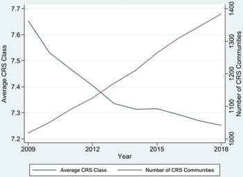
Count of CRS communities and average CRS class over time. Note: This figure shows the number of CRS communities and their average class rank over time.

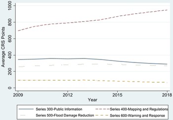
Average CRS points earned by category over time. Note: This figure shows the average annual CRS points earned from different category of CRS activities over time.

Annual premium by CRS status. Note: This figure shows the average annual premium by CRS participants and non-CRS participants over time.

Policies in force by CRS status. Note: This figure shows the number of policies in force in CRS and non-CRS communities over time.

Geographical weight. Note: This figure shows the intersection result example of census block group map and CRS community map. Autauga County (CID:010314) and City of Prattville (CID:010002) are two CRS communities with black border line. Census block groups are polygons with yellow border line. The highlighted area with blue border line is the intersected area between census block group: 010010201001 with two CRS communities mentioned above. The area of the intersected region is 4.276222, and the areas of the intersected regions with Autauga County and City of Prattville are 0.917327 and 3.256695, respectively. Then census block group: 010010201001 contributes 21.5% to Autauga County and 78.5% to City of Prattville when calculating total population or number of policy of that community.

Distribution of premium differences over household income. Note: The figure shows statistics describing the distribution of the ratio of premium differences over household income. The premium differences are produced by subtracting baseline premiums, those without CRS adjustments, from those that include the CRS adjustments. The ratios are calculated at community level.

Impact of HMA grants on CRS outcomes using initial approval date

Note: This table reports results based on the same specifications as those in Table 9, but here we use Initial Approval Date as to specify the year in which the community received the funds. All models include state and year-fixed effects. Robust standard errors are in parentheses. ${{\rm{\;}}^{{\rm{***}}}}p$
< 0.001,
${{\rm{\;}}^{{\rm{***}}}}p$
< 0.001, ${{\rm{\;}}^{{\rm{**}}}}p $
< 0.01,
${{\rm{\;}}^{{\rm{**}}}}p $
< 0.01, ${{\rm{\;}}^{\rm{*}}}p$
< 0.05.
${{\rm{\;}}^{\rm{*}}}p$
< 0.05.
Impact of HMA grant on CRS points by activity level

Note: This table shows results for the impact of HMA grants on CRS points earned by activity level. CRS points are measured in 100s. The levels are shown above the columns; the definitions are shown in Table 1. Part A. shows results for the HMA indicator variable, and Part B. shows results for HMA defined based on dollars received. All models include state and year-fixed effects as well as a full set of demographic variables. Robust standard errors are in parentheses. ${{\rm{\;}}^{{\rm{***}}}}p $
< 0.001,
${{\rm{\;}}^{{\rm{***}}}}p $
< 0.001, ${{\rm{\;}}^{{\rm{**}}}}p$
< 0.01,
${{\rm{\;}}^{{\rm{**}}}}p$
< 0.01, ${{\rm{\;}}^{\rm{*}}}p$
< 0.05.
${{\rm{\;}}^{\rm{*}}}p$
< 0.05.
Impact of HMA grants on CRS outcomes using restricted samples

Note: All models include state and year-fixed effects as well as a full set of demographic variables. Robust standard errors are in parentheses. ${{\rm{\;}}^{{\rm{***}}}}p$
< 0.001,
${{\rm{\;}}^{{\rm{***}}}}p$
< 0.001, ${{\rm{\;}}^{{\rm{**}}}}p$
< 0.01,
${{\rm{\;}}^{{\rm{**}}}}p$
< 0.01, ${{\rm{\;}}^{\rm{*}}}p $
< 0.05.
${{\rm{\;}}^{\rm{*}}}p $
< 0.05.


 Open access