


1. INTRODUCTION
Establishing records of glacier change is important for understanding how the cryosphere responds to natural and anthropogenic climate change. Glaciers respond to multiple climatic conditions on intraannual to decadal timescales. Therefore, chronologies of past glacier volume, length, equilibrium line altitude (ELA), and mass balance provide a valuable means for developing and testing predictive models, as well as environmental evidence that help us understand how past climate variability and change impacted glacial systems. From this understanding, we can better evaluate how glaciers will change in the future.
The Randolph Glacier Inventory (RGI Consortium, 2017) includes the location and elevation of most of the worlds glaciers, as well as mass balance, ELA, and length changes for glaciers that have been more thoroughly studied. Included in that database are the >3100 glaciers in Southern Alps of New Zealand. These New Zealand glaciers were inventoried in 1978, at which time they had an area of ~1160 km2 (Chinn, Reference Chinn2001; Radić and Hock, Reference Radić and Hock2010). New Zealand glaciers are characterized by high precipitation, over 10 m water equivalent (w.e.) per year in some locations, due to prevailing westerly winds and orographically enhanced precipitation (Henderson and Thompson, Reference Henderson and Thompson1999). The high precipitation and low elevation of Southern Alps termini results in glaciers with a high-mass turnover and a high sensitivity to climatic perturbations (Oerlemans and Fortuin, Reference Oerlemans and Fortuin1992; Anderson and Mackintosh, Reference Anderson and Mackintosh2012). New Zealand glaciers make up a small percentage Earth's glaciers and contain only 0.21 mm of global sea level equivalent (Radić and Hock, Reference Radić and Hock2010). However, their response to South Pacific climate variations is important for understanding the relationship between glaciers and regional climate variability (Mackintosh and others, Reference Mackintosh2017). Additionally, their high sensitivity to climate makes them excellent indicators of climatic changes (Oerlemans, Reference Oerlemans1994), and their location provides one of the few Southern Hemisphere records of maritime glacier variability (e.g. Oerlemans, Reference Oerlemans2005; Schaefer and others, Reference Schaefer2009).
A subset of 50 New Zealand glaciers have been monitored since 1977 as a part of the end-of-summer-snowline (EoSS) survey (Fig. 1a). The EoSS can be visually identified as the highest elevation of bare or exposed glacier ice or firn and, assuming that all meltwater refrozen during the previous winter has melted during the ablation season, the EoSS can be used as a proxy for the annual ELA (LaChapelle, Reference LaChapelle1962; Oerlemans, Reference Oerlemans2010; Chinn and others, Reference Chinn, Fitzharris, Willsman and Salinger2012). This assumption has been made for New Zealand glaciers before (Chinn and others, Reference Chinn, Winkler, Salinger and Haakensen2005, Reference Chinn, Fitzharris, Willsman and Salinger2012), and is again made in this study. EoSS surveys involve taking hand-held oblique photographs of Southern Alps glaciers from a light aircraft to capture the snowline at the end of the glacier mass-balance year (March–April). Until now, ELAs were calculated by either: (1) manually transcribing the snowline from oblique photographs onto a base map, digitizing the maps, and using the total ablation area and the glacier's area–altitude curve to calculate the mean ELA; (2) visually arranging images for all years by decreasing snow cover, allowing a visual comparison and ELA estimate to be made based on the entire historic sequence; or (3) when the snowline is not visible or clear in the image, following the same steps as in (2), but comparing the size of annual snow patches surrounding each glacier (Willsman and others, Reference Willsman, Chinn and Macara2015). All of these approaches are qualitative, and therefore have a relatively low repeatability and provide little transparency about how past ELAs were initially determined. Additionally, these approaches do not contain clear estimates of error for how each photograph and snowline was evaluated.

Fig. 1. (a) Glaciers located on the South Island of New Zealand (blue) (WGMS, 2017), the 50 New Zealand index glaciers included in the EoSS survey (white), Brewster Glacier (red), Fox Glacier/Te Moeka o Tuawe (green), and Franz Josef Glacier/Kā Roimata o Hine Hukatere (orange). (b) Orthophoto with GCPs (yellow) and (c) DEM of Brewster Glacier from 11 March 2016 produced using structure from motion photogrammetry. Both have a resolution of 0.26 m.
We have established a technique whereby we use structure from motion photogrammetry (SfMP) to revisit the historical EoSS photographs and quantitatively measure past glacier fluctuations. Previous works have successfully used SfMP in Earth science research, including to quantify changes in snow depth, and glacier volume and mass balance (Westoby and others, Reference Westoby, Brasington, Glasser, Hambrey and Reynolds2012; Nolan and others, Reference Nolan, Larsen and Sturm2015; Piermattei and others, Reference Piermattei, Carturan and Guarnieri2015). SfMP uses multiple overlapping images, georeferenced either with ground control points (GCPs) or camera coordinates for each image, and feature-matching algorithms to generate a three-dimensional (3-D) point cloud of the glacier. The point cloud is a set of (X,Y,Z) points defining the glacier surface, which are then interpolated to produce DEMs and orthophoto mosaics of the glacier. In addition to the geometry of the glacier, SfMP solves for the interior (principal point and focal length) and exterior (position and orientation) camera parameters, making it possible to use a set of modern georeferenced images to determine the locations from which the historic EoSS images were taken.
Here we use the SfMP method to quantitatively measure terminus positions and annual ELAs from historic images of one EoSS glacier, Brewster Glacier (Fig. 1), for which a set of historic images has been captured. Application of this method will enable others to revisit historic photographs of glaciers and use the images to quantitatively measure glacier change. Our three main objectives are to: (1) investigate the accuracy of georeferencing image locations, using Global Navigation Satellite System (GNSS) and a precise equipment timer (PET), for SfMP models; (2) identify the ELA and terminus position in georeferenced historic images and assess the uncertainty of this methodology. These uncertainties are mainly due to (i) the interior and exterior camera parameters of the historic images calculated using the SfMP algorithms, (ii) the back-projection of the ELA image coordinates into real world coordinates using digital elevation models (DEMs), and (iii) the auto-identification of the terminus position in historic images; (3) compare the SfMP-derived ELA and length records for Brewster Glacier with previous measurements of mass balance and terminus positions.
2. STUDY SITE
Brewster Glacier is located to the west of the Southern Alps main drainage divide at 44.08°S, 169.43°E. The glacier has a surface area of ~2 km2 and spans an elevation of 1670–2400 m a.s.l. An automatic weather station installed in front of the glacier at 1650 m a.s.l. from 2004 through 2008 measured mean annual near-surface air temperature of 2.5°C and annual precipitation of 5.3 m (Anderson and others, Reference Anderson2010). Brewster Glacier snowlines have been photographed during 36 of the past 40 years (1978–2017), and have been used as a mass-balance proxy. ELAs estimated from images of snowlines suggest that the glacier has been in a positive balance for 21 of the 38 years (1978–2015), but has been in mostly negative mass balance since 2008 (Willsman and others, Reference Willsman, Chinn and Macara2015). Brewster Glacier ELAs are shown to have a correlation of 0.83 with mean ELAs for all 50 EoSS glaciers, indicating that Brewster ELA fluctuations are representative of ELA fluctuations in the Southern Alps (Willsman and others, Reference Willsman, Chinn and Macara2015).
Brewster Glacier has been extensively monitored and studied in addition to the EoSS survey. Mass balance has been monitored since 2004, with measurements showing years with high positive net balances and years with high negative net balances (Stumm, Reference Stumm2011; Cullen and others, Reference Cullen2017). Modeling results indicate that Brewster mass balance is extremely sensitive to changes in temperature and that even moderate temperature increases could lead to significant ice loss (Anderson and others, Reference Anderson2010). Additional unpublished data from Brewster includes terminus positions recorded by GNSS foot surveys between 12 March and 20 April every year since 2005, with an exception in 2006 when the survey was taken on 20 January. GNSS foot surveys of the glacier surface elevation have also been collected in 1997, 2005, and 2008–16.
3. METHODOLOGY
To develop Brewster length and ELA records, we use historic annual images, a large dataset of georeferenced images taken in 2017, and modern and historic DEMs of the glacier. Following data acquisition, the snow and ice in all images are masked out and, using the SfMP software AgiSoft PhotoScan, the images are oriented to generate a base map of the bedrock surrounding the glacier. Having the georeferenced 2017 images makes it possible to calculate interior and exterior parameters for the historic images, which are then used to calculate ELAs and terminus positions. Figure 2 shows an overview of the data acquisition and processing methodology, which is detailed below.
Fig. 2. An overview of the workflow used to calculate glacier length and ELA from historic images, with the inputs for the transformations and back-projection shown in italics.
3.1. Data acquisition
3.1.1. EoSS images
While the first EoSS images of Brewster Glacier were taken in 1978, we use images starting in 1981. This is because the images from 1978 were taken far from the glacier, resulting in high errors in the SfMP-calculated camera parameters, no images were taken in 1979, and clouds obscured the glacier in 1980. This results in 200 images of Brewster Glacier from 1981 to 2014 (Table 1), which we refer to as historic images. There is year-to-year variability in the types of cameras used to obtain historic glacier imagery. Single-lens reflex (SLR) film cameras were used prior to 2009, and digital cameras (Sony DSC-W50, Pentax K100D, Nikon D200) were used from 2005 to 2014 (Table 1). For historical imagery in analog format, all EoSS slides and film strips were digitally scanned and archived in 2015–17 using a Hasselblad X5 high-resolution drum scanner. The only metadata available for these images is the date they were taken.
Table 1. Details of historic (1981–2014) and modern (2015–17) images taken of Brewster Glacier annually, including the number of film images, number of digital images, and type of digital SLR used
a No images taken in 1990 or 1991.
b 118 images taken 11 March 2016 and 195 images taken 30 March 2016.
3.1.2. Modern georeferenced image acquisition
Starting with the 2015 EoSS flight, a larger number of digital images (>60, referred to as modern images) were taken by hand and georeferenced (Table 1) specifically for (1) generating high-resolution modern DEMs and orthophotos, and (2) determining the interior and exterior camera parameters of historic images using SfMP. Oblique photographs were taken manually using a Nikon D800E camera while the aircraft circled the glacier. The camera is a 36.3 megapixel professional-grade full-frame digital SLR camera. A Nikon 50 mm lens was used in 2015, and a Nikon 85 mm lens in 2016 and 2017. This focal length, which may not be optimal for Brewster Glacier, was selected to best photograph all EoSS glaciers, and is within the range suggested in Mosbrucker and others (Reference Mosbrucker, Major, Spicer and Pitlick2017). The focus was fixed at infinity while taking photos.
To determine positions of images taken during the flights, a dual frequency GNSS receiver was mounted in the aircraft. On the 2015 and 2016 flights, we used a Trimble GeoXH GNSS receiver with positions logged at 1 s intervals. The data were post-processed using Trimble Pathfinder Office against a network of base stations located near the study site that also logged data at 1 s intervals, the closest sites being Makarora (24 km) and Haast (52 km). On 30 March 2016, we also used a Trimble R8 GNSS receiver with positions logged at 1 s intervals. The data were post-processed using Canadian Spatial Reference System Precise Point Positioning (Natural Resources Canada, 2016). On the 2017 flight, we used a Septentrio PolaRx5, sampling at 1 and 0.1 s intervals, and post-processed using Canadian Spatial Reference System Precise Point Positioning (Natural Resources Canada, 2016).
One of the uncertainties in image positions is associated with timing. The Nikon D800E records the time of digitization at 0.1 s resolution, but as the aircraft's average speed over Brewster Glacier is c. 70 m s−1, we can only estimate image position within 7 m. Camera-GNSS synchronization was done in 2016 and 2017 using a PET to capture the image timing at the millisecond level. The PET is a GNSS-synchronized timer connected to the flash synchronization connector on the camera that records the time of image acquisition at better than 1 × 10⁻³ s resolution. This enhanced temporal resolution makes it possible to reduce the timing component of the image position error to c. 0.07 m.
3.1.3. Field data
Field data were acquired in March 2016 in order to georeference and validate our SfMP models. We collected 10 GCPs from bedrock around Brewster Glacier. The GCPs, easily visible in the modern and historic aerial images, are used to georeference the models and are used as check points in order to assess the accuracy of the models. GCPs were collected using the Trimble R8 receiver, logging at 1 s intervals, and post-processed using Canadian Spatial Reference System Precise Point Positioning (Natural Resources Canada, 2016). A surface elevation survey of the glacier was conducted on 25–27 March 2016 using the Trimble R8 receiver, and the data were also post-processed also using Canadian Spatial Reference System Precise Point Positioning (Natural Resources Canada, 2016).
3.1.4. Historic DEMs
The calculation of ELAs from historic photographs uses the surface elevation of the glacier. As the glacier surface elevation is not constant over the 40-year period, we use DEMs spanning the period of the chronology (Table 2) that were developed by Thornton (Reference Thornton2017), instead of exclusively using the 2017 DEM generated from SfMP. The 1967 and 1986 DEMs are derived from New Zealand topographic maps, the 2000 DEM is from the Satellite Radar Topography Mission (SRTM; Reuter and others, Reference Reuter, Nelson and Jarvis2007), and the other DEMs were generated from annual GNSS foot surveys of the glacier surface and then interpolated using the co-kriging approach (Goovaerts, Reference Goovaerts1998; Thornton, Reference Thornton2017). The vertical errors for the 1967, 1986, and 1997 DEMs are calculated as one standard deviation (std dev.) of the difference between the ice-free parts of each of these DEMs and the 2017 SfMP DEM, which is assumed to have a 0 m error. The vertical errors for DEMs generated from the foot surveys are calculated as the mean standard error from the co-kriging approach. The error is inversely proportional to the number of GNSS points and the coverage of points, with the low error in 1997 due to almost full coverage of the glacier surface (Thornton, Reference Thornton2017).
Table 2. Brewster Glacier DEMs used to calculate ELAs, including the vertical error and source for each
3.2. SfMP processing
3.2.1. Modern DEMs and orthophotos
We use SfMP and the large dataset of georeferenced images taken between 2015 and 2017 to generate high-resolution DEMs and orthophotos for each of these years. The SfMP models are georeferenced with camera locations and five of the GCPs, with the other five used as check points. Each of the GCPs are manually identified when visible in an image. The workflow that results in the lowest model RMSE when building the point cloud is: (1) set the camera location accuracy to 0.1 m, GCP accuracy to 0.005 m, and define the coordinate system; (2) match and align cameras; (3) import camera locations and GCPs; (4) repeat alignment. After building the point cloud, the workflow includes generating a dense cloud and model, all with the following settings. The point cloud alignment settings include ‘high’ accuracy, pair preselection disabled, key point limit of 100 000 and tie point limit of 6000, and adaptive camera model fitting enabled. The dense cloud settings include ‘high’ accuracy and ‘moderate’ depth filtering. The model settings include height field surface type, dense cloud source data, interpolation disabled, ‘high’ face count, generic mapping mode, mosaic blending mode, texture size of 4096 × 4096, color correction disabled, and hole filling enabled. For each year, the same set of interior camera parameters, determined by the SfMP software, are used for all images.
3.2.2. Determining historic camera parameters
Interior and exterior camera parameters, including image position, are determined using AgiSoft PhotoScan software, which includes a SfMP algorithm (Koenderink and van Doorn, Reference Koenderink and van Doorn1991; Westoby and others, Reference Westoby, Brasington, Glasser, Hambrey and Reynolds2012). We tested three different methods to identify the best for processing of the historic images, with the following method resulting in the most historic images oriented with the point cloud, and the most accurate camera parameters (determined using GCPs). We generate one SfMP point cloud of only the bedrock surrounding Brewster Glacier. This is generated using the 192 images taken in March 2017 and all 200 historic Brewster EoSS images. The model is georeferenced with the 2017 camera positions and five of the GCPs, with the other five used as check points. The same set of interior camera parameters, determined by the SfMP software, are used for all 2017 images. Snow and ice are masked out of all images, historic and modern, using a modified form of the Otsu (Reference Otsu1975) thresholding method to distinguish snow and ice from the bedrock. This is done because snow and ice vary annually, while we assume that the bedrock is stable and can therefore be used to orient all images over the 40-year period. The SfMP algorithm matches points in the bedrock of the historic images with the 2017 images in order to orient the historic images and calculate the camera parameters, including the position from which the images were taken. The point cloud alignment settings include ‘high’ accuracy, pair preselection disabled, key point limit of 200 000 and tie point limit of 15 000, and adaptive camera model fitting enabled. Historic images without enough common features to be identified by the SfMP software, due to the presence of cloud cover or little bedrock in the images, do not orient in the model and therefore the camera parameters cannot be calculated.
We note that this workflow, of using SfMP to calculate camera parameters for historic images and then using that information in the transformations and back-projection, is necessary for working with these EoSS image datasets. This is because there are multiple years for which only one image of the terminus or ELA exists for Brewster Glacier (Table 1). However, for years with multiple images of each part of the glacier, the following SfMP workflow is also possible: (1) orient all masked images (historic and modern), (2) disable all photos except those from a single year, (3) build a dense cloud, DEM, and orthophoto for that year. Here, we exclusively use the back-projection method to keep the ELA and length calculations consistent.
3.3. Snowline and terminus position selection
To identify snowlines and terminus positions in photographs, all images are enhanced using the contrast limited adaptive histogram equalization (Pizer and others, Reference Pizer1987). This increases the contrast within subregions of the images and enhances the difference between ice and snow on the glacier, especially helping with identification of the snowline (Fig. 3). The snowline is identified as the highest elevation of exposed glacier ice or firn (LaChapelle, Reference LaChapelle1962; Oerlemans, Reference Oerlemans2010), and is manually digitized for each image. Identification of terminus positions is automated by thresholding pixel values. Grayscale pixel intensity values for each EoSS image are used to identify the minimum and maximum pixel value thresholds, resulting in discrimination of the glacier from bedrock (Fig. 3b).

Fig. 3. Example scanned EoSS image from 1995, (a) original and (b) enhanced by contrast limited adaptive histogram equalization, with the terminus position (gray) identified using pixel thresholding, and the snowline (blue) manually digitized.
3.4. Transformations
In order to determine the real world positions in the New Zealand Transverse Mercator (NZTM) projection from image (x, y) coordinates of snowlines and terminus positions, transformations of image geometry and conversions of (x, y) image coordinates to real-world (NZTM) coordinates are performed. These steps are fully described in the Appendix. Using a standard ideal camera model that considers interior camera parameters (Ma and others, Reference Ma, Soatto, Kosecka and Sastry2012), we calculate the relationship between glacier features in the real world and pixels in an image. Lens distortion is corrected for, with total distortion calculated as the combination of radial distortion and tangential (decentering) distortion. We then complete a back-projection, calculating the position of snowline and terminus (x, y) image coordinates in real-world (NZTM) coordinates. The back-projection uses the interior and exterior camera parameters, a DEM of the glacier surface, and (x, y) image coordinates of snowlines and termini. The real-world (NZTM) coordinates of an image pixel are calculated by intersecting a ray from the camera location with a DEM, and using a stepping scheme to calculate the intersection point.
3.5. Calculating uncertainties and compiling chronologies
3.5.1. ELA uncertainties
Uncertainty in the ELA comes from (1) errors in the DEMs used in the back-projection and (2) errors in the SfMP-calculated camera interior and exterior parameters. We use DEMs spanning the period of the chronology (Table 2) to calculate ELAs. For years with no DEM, we use the closest previous year and later year with DEMs to interpolate annual glacier surfaces. This method of using distinct DEMs in the snowline back-projection for each year (1981–2014) accounts for changes in the glacier surface over time.
We calculate the uncertainties in ELAs due to the DEMs used in the back-projection (E D). For each DEM in Table 2, we add the vertical error to the glacier surface to represent the maximum possible surface elevation. Again, for years with no DEMs, we interpolate the glacier surface for each year. We repeat the back-projection and calculate ELAs using these maximum surface elevations (S Dh). These steps are then repeated for the minimum surface elevations by subtracting the vertical error from each DEM surface and calculating ELAs using these minimum surface elevations (S Dl). We calculate the differences between the ELAs calculated using the non-adjusted surface elevations (S D) and ELAs calculated using the minimum and maximum surface elevations, and use the largest absolute difference to represent the uncertainties in each ELA from DEMs, so that E D is equal to the the largest error between |S D − S Dh| and |S D − S Dl|. For each image, the calculated E D is between 0 and 30 m, with a mean value of 5 m. E D is larger for images towards the beginning of the chronology, when the vertical DEM errors are largest. ELAs with E D over 10 m correspond to ELAs higher than 2150 m a.s.l. This is due to the slope of the glacier being steepest above 2100 m a.s.l., leading to larger differences in ELAs back-projected onto the non-adjusted, minimum, and maximum surface elevations.
In order to assess the accuracy of the camera positions, we use the previously described GCPs. Two GCPs, selected as the easiest to accurately identify in images, were located in each historic image in which they were present. The GCP (x, y) points selected in each image were back-projected following the same steps as the snowlines and terminus positions. For each image with a GCP, the horizontal distance between the back-projected point and the coordinates of the GCP was calculated and considered to be representative of the back-projection and camera parameter uncertainty for that image. The distances are averaged for images with the two GCPs, and considered to be the horizontal error for each image (E hG). Images with no visible GCP (36 of the 200 historic images), due to image coverage, cloud cover, or image resolution, were not used in the chronologies.
As the DEM uncertainty is represented by vertical error, we use this horizontal GCP error and the glacier slope to calculate the associated vertical GCP error. Using the 2017 SfMP DEM, we calculate the mean slope of the entire glacier (21.2°) and the mean slope of the accumulation area (34.6°), where the glacier is the steepest. We use the slope of the accumulation area to provide an upper estimate, and calculate the vertical GCP error (E
vG) following E
vG = E
hG · tan(34.6°). The total uncertainty of each ELA (E
S) includes errors from the DEM used (E
D) and the vertical error from the camera parameters, calculated using GCPs (E
vG), and is calculated following $E_{{\rm S}} =\sqrt {(E_{{\rm D}})^{2}+(E_{{\rm vG}})^{2}}$
. To compile the chronology, we calculate each ELA as the mean elevation of the digitized points. For years with only one image of the snowline, the calculated ELA and corresponding error (E
S) are used in the chronology. For a year with multiple images, we first select all individual ELAs with a vertical GCP error (E
vG) under 24 m. If the year had no ELA with E
vG under 24 m, the threshold is increased to 69 m and all ELAs with E
vG below that value were selected. The thresholds are determined by visually analyzing the data to exclude images with high errors while still including most images. We set thresholds using E
vG instead of E
D or E
S because E
D are relatively consistent for all ELAs, while E
vG can vary between 0 and 100 m depending on the accuracy of the calculated camera parameters. We use this thresholding step to eliminate ELAs calculated from images with high errors in the calculated camera parameters. When this thresholding of uncertainties results in years with multiple ELAs (due to multiple images), we calculate the weighted mean and resulting uncertainties to determine the mean annual ELA.
$E_{{\rm S}} =\sqrt {(E_{{\rm D}})^{2}+(E_{{\rm vG}})^{2}}$
. To compile the chronology, we calculate each ELA as the mean elevation of the digitized points. For years with only one image of the snowline, the calculated ELA and corresponding error (E
S) are used in the chronology. For a year with multiple images, we first select all individual ELAs with a vertical GCP error (E
vG) under 24 m. If the year had no ELA with E
vG under 24 m, the threshold is increased to 69 m and all ELAs with E
vG below that value were selected. The thresholds are determined by visually analyzing the data to exclude images with high errors while still including most images. We set thresholds using E
vG instead of E
D or E
S because E
D are relatively consistent for all ELAs, while E
vG can vary between 0 and 100 m depending on the accuracy of the calculated camera parameters. We use this thresholding step to eliminate ELAs calculated from images with high errors in the calculated camera parameters. When this thresholding of uncertainties results in years with multiple ELAs (due to multiple images), we calculate the weighted mean and resulting uncertainties to determine the mean annual ELA.
3.5.2. Length record
We calculate glacier length, following (Purdie and others, Reference Purdie2014), as the furthest connected ice at the terminus perpendicular to the centerline, defined by the mass-balance program (Cullen and others, Reference Cullen2017). We use the 2017 SfMP DEM for all terminus back-projections and do not consider E D, as the RMSE of the DEM is ~0.5 m. We can use the 2017 DEM instead of annual DEMs for the terminus back-projection because the terminus is always being identified as the furthest point on the glacier, and as 2017 is the shortest glacier extent in the chronology, the terminus position is always being projected onto bedrock. We calculate E hG for each terminus position in the same way it was calculated for ELAs.
We also estimate the error associated with the automated terminus identification (E
a
). This was done by selecting a subset of images and determining the variation in the identified terminus position. All variation fell between ± 15 m, so for each terminus position E
a is 15 m. The total uncertainties in each terminus position (E
T) are calculated following $E_{{\rm T}}=\sqrt {(E_{{\rm hG}})^{2} + (E_{{\rm a}})^{2}}$
. For years with only one image of the terminus position, the calculated length and corresponding error (E
T) are used in the chronology. For a year with multiple images of the glacier terminus, we select all terminus positions with E
hG below 35 m, and if the year has no terminus positions below that error, the threshold is increased to 90 m. Again, thresholds are determined by visually analyzing the data to exclude images with high errors while still including most images. We then further filter the terminus positions by calculating the mean length (
$E_{{\rm T}}=\sqrt {(E_{{\rm hG}})^{2} + (E_{{\rm a}})^{2}}$
. For years with only one image of the terminus position, the calculated length and corresponding error (E
T) are used in the chronology. For a year with multiple images of the glacier terminus, we select all terminus positions with E
hG below 35 m, and if the year has no terminus positions below that error, the threshold is increased to 90 m. Again, thresholds are determined by visually analyzing the data to exclude images with high errors while still including most images. We then further filter the terminus positions by calculating the mean length ( ${\bar L}_{i}$
) and std dev. (σ
i
) for a year. For each year (i), each calculated length for that year that falls outside of
${\bar L}_{i}$
) and std dev. (σ
i
) for a year. For each year (i), each calculated length for that year that falls outside of ${\bar L}_{i} \pm \sigma _{i}$
is not considered. This is done to discard lengths calculated from images for which the automated terminus identification may have incorrectly selected a feature, including shadows on ice, clouds, or water. We then calculate the weighted mean of the positions for each year to determine annual length and resulting uncertainties.
${\bar L}_{i} \pm \sigma _{i}$
is not considered. This is done to discard lengths calculated from images for which the automated terminus identification may have incorrectly selected a feature, including shadows on ice, clouds, or water. We then calculate the weighted mean of the positions for each year to determine annual length and resulting uncertainties.
4. RESULTS AND DISCUSSION
4.1. Modern SfMP models
We first show that it is possible to produce a high-accuracy SfMP modern model of Brewster Glacier with georeferenced images, with and without GCPs (Table 3). We generate SfMP models of Brewster Glacier from images taken between 2015 and 2017, and test the accuracy of georeferencing the models with camera locations only (acquired with and without the PET), GCPs only, and both camera locations and GCPs. When using only camera locations for georeferencing, we use all 10 GCPs as check points, and when georeferencing with GCPs (with and without camera locations), we use five of the GCPs as check points and the other five for georeferencing. Check points are not used to georeference the model, and instead give an idea of the true model error as the mean distance between GNSS-measured GCPs and the position of the GCPs in the SfMP model.
Table 3. Details and accuracy of the 2015–17 SfMP models. Model RMSE is reported for georeferencing using (1) GCPs and camera locations, (2) GCPs only, and (3) camera locations only. For 1 and 2, we report the GCP check error, determined using five of the 10 GCPs not used to georeference the model but only used to estimate the true model error. For 3, we report the camera location error and the GCP check error, determined from all 10 GCPs
The camera location RMSE is the mean distance between sampled GNSS (X, Y, Z) image locations (acquired with and without the PET) and the (X, Y, Z) image locations calculated by the SfMP software. We show that using the PET, on 11 March 2016 and 9 March 2017, the camera location RMSE is reduced to 0.73 and 0.61 m, respectively (Table 3). For the 2017 model, the GCP check point RMSE is 0.85 m, showing that we can georeference SfMP models exclusively with camera locations with accuracies under 1 m. However, the GCP check point RMSE for the 2016 model is about double the camera location error, suggesting that the larger dataset of images acquired in 2017 (192 images) compared with 2016 (118 images) may help to improve model accuracy when using the PET and camera positions.
For all models, using only GCPs for georeferencing improves model error compared with using only camera locations (Table 3). However, future work includes applying this method to the additional 49 EoSS glaciers. Therefore, accurate georeferencing of the SfMP models exclusively using camera positions makes the development of additional glacier chronologies possible without having to collect GCPs in the field at all glaciers. Two limitations of the acquisition of modern images that we do not account for include the offset between the GNSS receiver and the position of the camera, and the distortions caused by taking images through the aircraft windows, which vary with each image. Accounting for this offset and distortion in the future would likely further decrease the model RMSE when georeferenced only with camera positions.
Comparison of the surface elevation survey, conducted 25–27 March 2016, with the SfMP DEM from 30 March 2016 shows that the two datasets are largely in agreement with each other and further validates the SfMP workflow for generating modern DEMs (Fig. 4). The mean difference between the two datasets is −0.0088 m, and the std dev. is 0.500 m. Some of the largest elevations differences, including the positive differences up to 2 m to the NE section of the survey, occur due to a step change in GNSS elevation of −1.8 m, possibly due to the loss of satellite coverage below Mt. Brewster to the NE. In addition, negative differences between the DEM and GNSS elevation are likely in part due to crevasses that are captured in the DEM, but stepped over during the foot survey. These results support our conclusion that it is possible to accurately map glaciers from an aircraft using SfMP without the need for GCPs.

Fig. 4. Comparison of 30 March 2016 SfMP Brewster Glacier DEM with the 25–27 March 2016 GNSS foot survey, with the frequency distribution of the elevation differences shown in the insert.
4.2. ELA record
We present ELAs from 1981 through 2017 calculated from historic oblique aerial images and SfMP orthophotos (Fig. 5, Table 4). Data are missing for 1982, 1984, and 1988 when snowlines were obscured by clouds, and 1990 and 1991 when no images were taken. Each annual ELA between 1981 and 2014 is calculated from between one and six historic images. The associated error includes the uncertainty in calculated camera parameters and back-projection, and the uncertainty in the DEMs used to represent the glacier surface. The 2015–17 ELAs are calculated from SfMP orthophotos and DEMs, with the errors from the SfMP models.
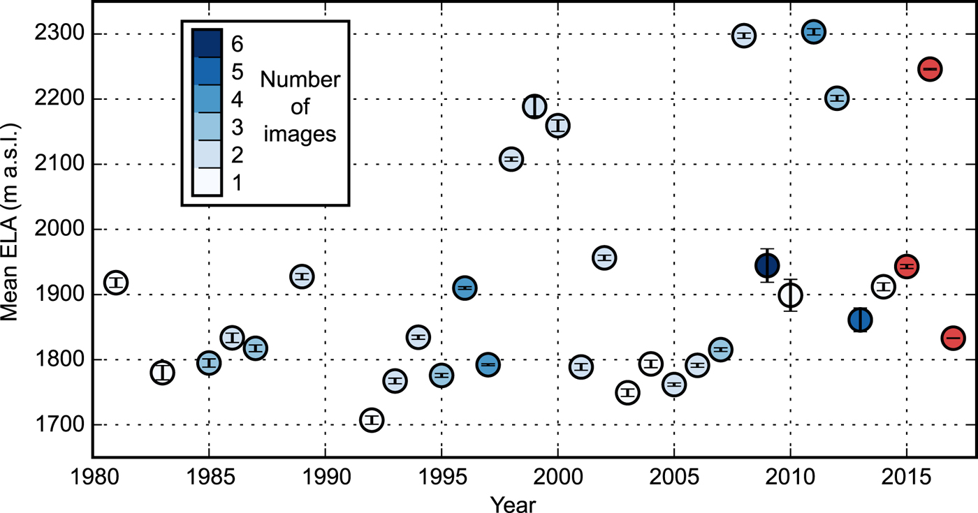
Fig. 5. Brewster Glacier mean ELAs 1981–2017 (cloudy or no images in 1982, 1984, 1988, 1990, and 1991). Each annual ELA (1981–2014) is calculated as the weighted mean of up to six historic images (shown with blue). The 2015–17 ELAs (red) were calculated from SfMP orthophotos and DEMs.
Table 4. Annual mean ELA, ELA range, and glacier length, 1981–2017
a 2015–17 ELAs and lengths calculated from SfMP orthophotos for each year.
The chronology shows the interannual variability in mean ELAs, with elevations ranging between 1707 ± 6 and 2303 ± 5 m a.s.l. Lower elevations occur in 1981–97 and in the early to mid-2000s, at the same time that many New Zealand glaciers were advancing (Purdie and others, Reference Purdie2014; WGMS, 2017). Higher ELAs occur in 1998–2000, and the highest occur more recently in 2008, 2011, 2012, and 2016.
Projection of equilibrium lines onto the 11 March 2016 SfMP orthophoto of Brewster Glacier shows a trimodal distribution (Fig. 6). The majority of equilibrium lines are either close to the terminus (a, 1700–1800 m a.s.l.), just below the steep accumulation area (b, 1900–1950 m a.s.l.), or at the top of the accumulation area (c, 2100–2300 m a.s.l.). No mean ELAs occur between ~1950 and 2100 m a.s.l. (Figs 5 and 6). This distribution is a result of the glacier geometry. Because of the low glacier gradient between areas (a) and (b), only a small difference in annual climate (temperature or snow cover) would drive the equilibrium line between the two areas of the glacier. This finding agrees with previous theoretical and observational work showing that glacier slope influences the sensitivity of glaciers to changes in climate, with gently sloping glaciers being more sensitive than steep glaciers (Oerlemans, Reference Oerlemans2001; Leclercq and others, Reference Leclercq2014).

Fig. 6. Brewster Glacier annual equilibrium lines (1981–2017) shown on the 11 March 2016 SfMP orthophoto. The equilibrium line with the lowest error was chosen for each year, with the earliest years shown in white, and the most recent years shown in dark blue. The are no equilibrium lines for 1982, 1984, 1988, 1990, and 1991. The gray lines are 50 m contours.
4.3. Comparison of SfMP–ELAs with previous ELA and mass-balance data
The extensive monitoring of Brewster Glacier makes it possible to compare our results with other work. Figure 7 shows the SfMP-calculated ELAs, the original ELA data, and the annual mass-balance measurements over the entire time series. ELAs are shown as the departure from the mean SfMP ELA (1919 m a.s.l.). Comparison of the SfMP-calculated ELA record and the original ELA data (Willsman and others, Reference Willsman, Chinn and Macara2015) shows that ELAs are within ± 100 m most years (Fig. 7), and the two datasets have an r 2 value of 90%. Differences between the ELA datasets are due to differences between the methods, or a human introduced bias in the selection of snowlines in images, not captured by our formal treatment of uncertainty. SfMP ELAs are calculated exclusively from digitizing snowlines on historic images, while the original ELA data were calculated by either (1) digitizing the accumulation or ablation area to identify the ELA, or by visually arranging images for all years by (2) decreasing snow cover or (3) snow patch size. We refer to ELAs calculated by step 1 as digitized ELAs, and ELAs calculated by steps 2 and 3 (these types are not differentiated by Willsman and others (Reference Willsman, Chinn and Macara2015)) as inferred ELAs. In addition to these differences in the method of calculating ELAs, the actual identification of the snowline from images contributes to the difference in the two chronologies. We identified snowlines as the highest visible ice or firn on the glacier, and all were identified by the same person to keep the data consistent.
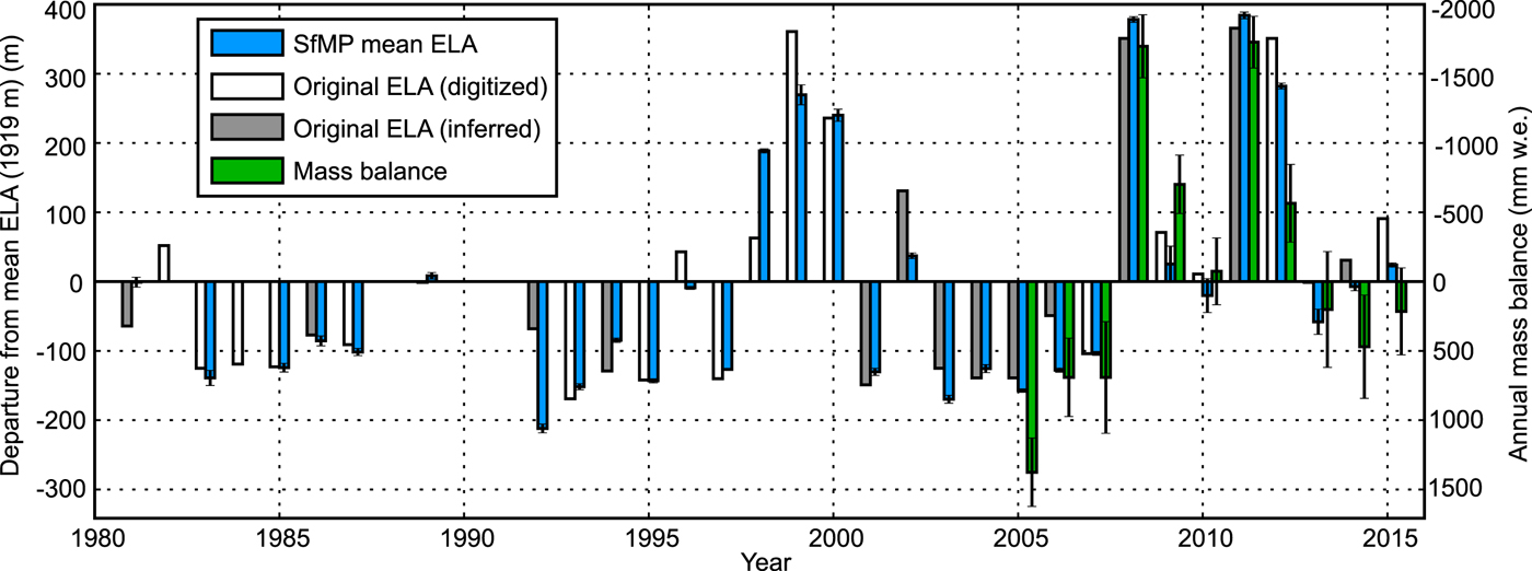
Fig. 7. Comparison of Brewster Glacier SfMP-calculated ELAs (blue) with associated errors, ELAs calculated using the original method, distinguished between digitized (white) and inferred ELAs (gray) (Willsman and others, Reference Willsman, Chinn and Macara2015), and annual mass balance (green) (Cullen and others, Reference Cullen2017). ELAs are shown as the departure from the mean SfMP ELA (1919 m a.s.l.). Note that an original ELA of 1918 m a.s.l. does exist for 1989.
Comparing ELAs with measured mass-balance data is important for understanding whether mass balance can be reconstructed from remote sensing methods. Figure 8a shows the relationship between Brewster Glacier ELAs calculated using SfMP and the mass-balance record (Cullen and others, Reference Cullen2017). The curve fit to the data has a gradual slope until the ELA reaches ~ 2000 m a.s.l. Above this elevation, the slope of the curve becomes steeper. This relationship suggests that due to the considerable increase in glacier slope at 2000 m a.s.l., the ELA becomes more sensitive, and a large change in ELA within this part of the glacier may correspond with a small change in mass balance. This finding is consistent with results from Cullen and others (Reference Cullen2017), which compared the same mass-balance data with the original ELA data. While the majority of years fall on or close to the curve fitting the data, 2009 and 2012 do not. In 2009, the ELA is within 10 m of the 2015 ELA, but 2009 was quite a negative mass-balance year (−702 mm. w.e.) while 2015 was slightly positive (215 mm w.e.) (Cullen and others, Reference Cullen2017). The EoSS survey in 2009 occurred 2 weeks before the mass-balance survey. There was no snowfall between the two surveys (Willsman and others, Reference Willsman, Chinn, Hendrikx and Lorrey2009), suggesting that additional ablation occurred after the snowline was photographed and before the mass-balance survey, and highlighting the importance of the timing of the EoSS and mass-balance surveys.
Fig. 8. Comparison of Brewster Glacier SfMP-calculated ELAs (2005–15) with (a) mass balance and (b) annual ELAs calculated from mass balance (Cullen and others, Reference Cullen2017).
Figure 8b shows the comparison of SfMP ELAs and ELAs calculated from mass balance. ELAs from mass balance were calculated by applying a geostatistical co-kriging approach to spatially adjust mass balance, and each annual ELA was interpolated between sampling elevations (Cullen and others, Reference Cullen2017). Within the errors of both datasets, the majority of years fall on the 1:1 ratio line, while 2006 and 2007 fall slightly below the line, and 2008 and 2012 are further above it. Comparison of ELAs calculated from mass balance and original ELA data (Willsman and others, Reference Willsman, Chinn and Macara2015) in Cullen and others (Reference Cullen2017) show a similar bias of 2007 falling below the 1:1 ratio line and 2008 and 2012 falling above it. These differences may be due to differences in the methods, with both methods having associated uncertainties. For example, the annual mass balance is almost identical for 2008 and 2011 (Fig. 8a), however, the ELAs calculated from mass balance for those years are over 200 m apart (Fig. 8b). Additional differences are likely due to differences in sampling time. For example, in 2008 the ELA calculated from mass balance, surveyed on 20 April, is almost 200 m lower than the SfMP ELA, photographed on 14 March. As the first winter snowfall usually occurs by early April (Willsman and others, Reference Willsman, Chinn and Macara2015), this suggests that snowfall occurred following the EoSS survey but before the mass-balance survey.
One source of differences between SfMP ELAs and mass-balance measurements arise from the timing of each monitoring program. The goal of the EoSS monitoring is to take images of the glaciers at the end of the melt season, and before any new snow has fallen. All flights for 2005–15 occurred between 3 and 15 March, with a supplemental flight in 2011 on 30 March after little to no snowfall following the first flight. However, ablation measurements for mass balance occurred over a longer window of time, between 13 February and 20 April. This means that in some years the two surveys are conducted within days of each other, while in other years the two surveys are over a month apart. In years when the two surveys are conducted at different times, there is the potential for additional melt between the two surveys, biasing the first survey toward lower ELAs or higher mass balance. There is also potential for new accumulation following the first survey, biasing the second survey toward lower ELAs or higher mass balance.
4.4. ELA uncertainties
The ELA record includes errors from the DEMs used to represent the glacier surface, and errors in the calculated camera parameters and back-projection. An additional source of unquantified uncertainty comes from the manual digitization of the snowlines from images. While the terminus selection is automated, we have not successfully automated the selection of the snowline. This is due to the small differences between snow and ice in some images, as well as some years when the previous year's firn is visible. To minimize this uncertainty, digitization was completed by one person to keep the selection consistent, and then reviewed and agreed upon among the authors. However, as some years do not have one clear snowline, there is uncertainty associated with this step. The uncertainty is greater when ELAs are above ~2100 m a.s.l., as this is the steepest part of the glacier and small differences in the selection of the snowline can lead to large differences in the resulting mean ELA.
Even when the snowline is perfectly identified in an image, for the EoSS to represent the ELA, images need to be captured at the end of the melt season but before any new snowfall. The timing of the flight is therefore chosen carefully each year, and there have been several years with multiple flights in order to capture the EoSS as accurately as possible. However, as there are years with snowfall before the flight and years with melt after the flight, the EoSS remains an imperfect proxy for the ELA.
We also investigate the influence of using historic DEMs in the ELA back-projection. ELAs calculated with DEMs for each year vary only slightly from ELAs calculated with the high-resolution and high-accuracy 2017 SfMP DEM. For each year in the chronology (1981–2014), we calculate S i, the difference between the ELAs calculated using the two different methods. We find that for all except 4 years, ELAs calculated with annual DEMs are higher in elevation than ELAs calculated with the 2017 DEM alone. For each year in the chronology, S i is between −31 m and +5 m, with a mean value of −11 m. S i correlates with the ELA, with more negative values for years with lower equilibrium lines, due to faster surface elevation lowering down-glacier compared with slower surface elevation loss of the accumulation area. S i is also more negative for years earlier in the chronology, when the difference between the year-of-interest DEM and the 2017 DEM is the greatest, and S i becomes less negative and slightly positive in the last decade of the chronology. These relatively small values of S i suggests that even when historical DEMs are not available for the back-projection, this method can be applied to calculate glacier fluctuations using a modern DEM and including this uncertainty.
4.5. Length record
Here we present the first annual Brewster Glacier length record extending through 1981 (Fig. 9, Table 4). Glacier lengths from 1981 through 2014 are calculated from historic images, and associated error includes the uncertainty in calculated camera parameters and back-projection, and in the automated terminus selection. Glacier lengths from 2015–17 are calculated from SfMP orthophotos, with errors from the respective SfMP models. The record shows 365 ± 12 m of terminus retreat since 1981, with significant retreat occurring 1981 through 1989, a period of slower retreat and slight advances between 1991–2008, and continuous retreat 2008–17.
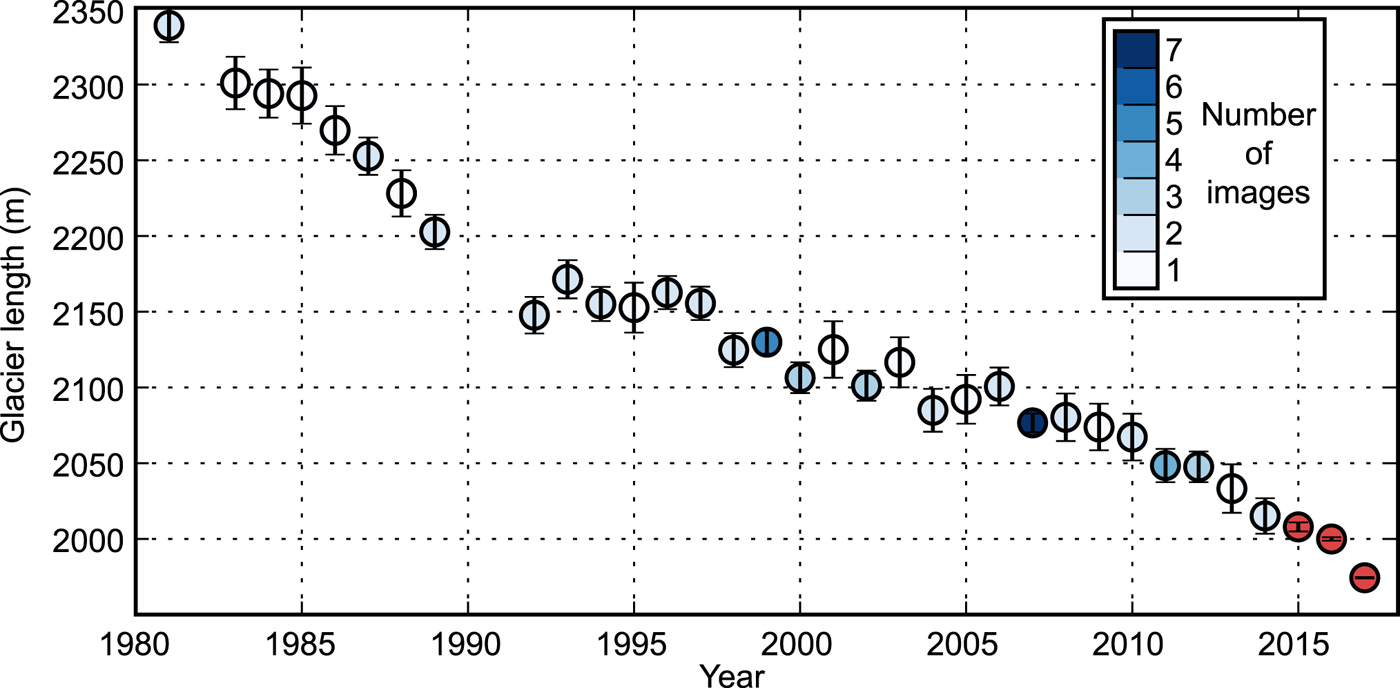
Fig. 9. Brewster Glacier lengths from 1981 through 2017 (no image match in 1982, and no images in 1990 and 1991). Each calculated length (1981–2014) is the weighted mean of up to seven images (shown with blues). The 2015–17 lengths (red) were calculated from SfMP orthophotos.
4.6. SfMP length record comparison with field data
We compare field measurements of terminus positions with our length measurements (2005–14) in Figure 10. All lengths match with the field measurements within uncertainties, except for 2005 and 2007. The 2005 and 2007 SfMP-calculated lengths underestimate the true glacier length because some historic images for those years were taken from angles that miss the furthest extent of the glacier, and were not recognized by the automated terminus identification. The match between the two length records shows that we can accurately calculate changes in glacier length from historic images. The difference in lengths in 2005 and 2007 demonstrates the need for more, higher quality images, and highlights the areas for improvement in the automated terminus identification.
Fig. 10. Brewster Glacier length time series (2005–14) compared with field measurements of the terminus position.
4.7. New Zealand glacier fluctuations
Comparison of Brewster Glacier length changes with fluctuations of New Zealand glaciers that have been more extensively studied help us to better understand Brewster Glacier dynamics. While most glaciers around the world have been retreating and losing mass since ~1950 (Zemp and others, Reference Zemp2015), a subset of New Zealand glaciers advanced between 1983 and 2008 (Purdie and others, Reference Purdie2014; WGMS, 2017). Of the New Zealand glaciers that advanced within that time, Fox Glacier/Te Moeka o Tuawe and Franz Josef Glacier/Kā Roimata o Hine Hukatere have been especially well monitored (Purdie and others, Reference Purdie2014). Both glaciers are longer than Brewster, at 12.4 and 9.9 km long, respectively, and are located 80–90 km northeast of Brewster. Fox Glacier/Te Moeka o Tuawe and Franz Josef Glacier/Kā Roimata o Hine Hukatere both react to climate variability within 3–4 years (Purdie and others, Reference Purdie2014), much faster than most valley glaciers, which react to climate variations in 10–50 years (Oerlemans, Reference Oerlemans1994). Both glaciers advanced from 1983 to 1999 and 2003 to 2007 in response to lower air temperatures (Mackintosh and others, Reference Mackintosh2017), but have been retreating quickly since 2011 (Fig. 11). In contrast, Brewster Glacier does not show the same length fluctuations, and instead experienced largely continuous retreat over the past 37 years (Fig. 11). This difference is due to Brewster Glacier responding more slowly to climate variability compared with Fox Glacier/Te Moeka o Tuawe and Franz Josef Glacier/Kā Roimata o Hine Hukatere. The slower response of Brewster Glacier is influenced by Brewster being a smaller glacier with a more gradual slope (Bahr and others, Reference Bahr, Pfeffer, Sassolas and Meier1998), and because Brewster has no steep, narrow glacier tongue, and therefore has a more even hypsometry compared with Fox Glacier/Te Moeka o Tuawe and Franz Josef Glacier/Kā Roimata o Hine Hukatere (McGrath and others, Reference McGrath, Sass, O'Neel, Arendt and Kienholz2017). Brewster Glacier response time, defined as the time to complete ~63% of its adjustment to a change in mass balance (Cuffey and Paterson, Reference Cuffey and Paterson2010), is calculated following Jóhannesson and others (Reference Jóhannesson, Raymond and Waddington1989) as 33 years (based on the 2017 thickness) to 43 years (based on the 1967 thickness) (Thornton, Reference Thornton2017). Because Brewster Glacier responds more slowly to climate variations, it is also likely that Brewster Glacier's retreat has been largely driven by 20th century warming and less by decadal climate variations that influence Fox Glacier/Te Moeka o Tuawe and Franz Josef Glacier/Kā Roimata o Hine Hukatere.
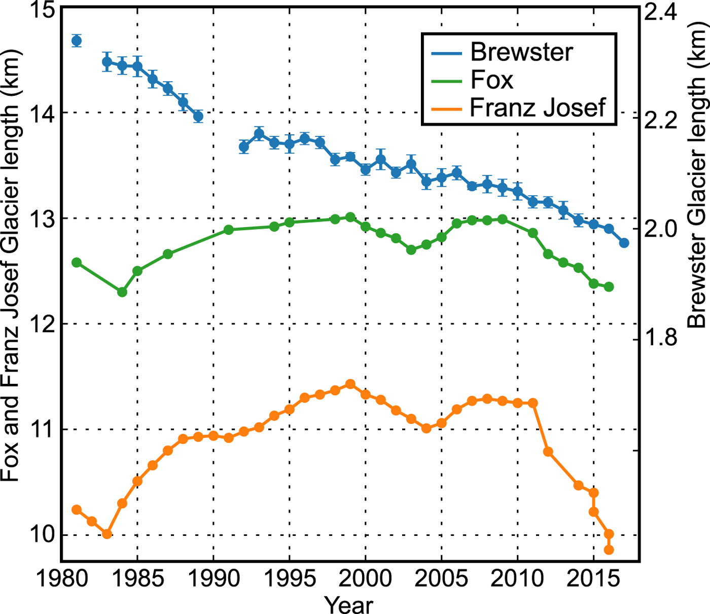
Fig. 11. Brewster Glacier length record (blue) compared with length records of Fox Glacier/Te Moeka o Tuawe (green) and Franz Josef Glacier/Kā Roimata o Hine Hukatere (orange) (Purdie and others, Reference Purdie2014).
5. CONCLUSIONS
We present a new method for quantitatively measuring glacier fluctuations from historic images, and detail the associated uncertainties. The method includes using modern georeferenced images and SfMP to determine the interior and exterior parameters of the historic images, including the location from which they were taken. We apply this method to Brewster Glacier, resulting in annual ELA and length records (1981–2017). Mean uncertainties associated with the method, quantified using GCPs, are 7 and 12 m for the ELA and length records, respectively. This method can be further applied to any glacier with historic images, and can be used to measure past changes in glacier width, area, and surface elevation in addition to ELA and length.
The Brewster Glacier ELA record shows pronounced interannual variability, with elevations between 1707 ± 6 and 2303 ± 5 m a.s.l. Lower ELAs occur in 1981–97 and in the early to mid-2000s, while the highest elevations occur more recently, in 1998–2000 and in 2008, 2011, 2012, and 2016. Our ELA record compares well with the original snowline elevation data for Brewster Glacier, and with measured mass-balance data (2005–15). Brewster Glacier's terminus retreated, largely continuously, 365 ± 12 m since 1981, with the most retreat occurring 1981–89, and more recently in 2008–17. Comparison with length variations of Fox Glacier/Te Moeka o Tuawe and Franz Josef Glacier/Kā Roimata o Hine Hukatere, shows that Brewster Glacier responds more slowly to climate variations, suggesting that Brewster retreat has been dominantly forced by 20th century warming.
Acknowledgments
This work was supported by the NIWA Strategic Science Investment Fund project Climate Present and Past, contracts CAOA1501, CAOA1601, CAOA1701, and CAOA1801, and the Victoria University of Wellington Doctoral Scholarship. We thank Trevor Chinn for pioneering and continuing the EoSS survey. We also thank two anonymous reviewers and editor, Hester Jiskoot, for their detailed and constructive comments.
APPENDIX A
A.1 Transformations
Determining the real world positions in the New Zealand Transverse Mercator (NZTM) projection from image (x, y) coordinates of snowlines and terminus positions, required several transformations. These transformations include from camera space to SfMP model space (T cm) and from model space to world space (NZTM) (T mw), as well as the inverses of both (T mc) and (T wm).
A.1.1. Camera model
The relationship between glacier features in the real world and pixels in an image is based on a standard ideal camera model (Ma and others, Reference Ma, Soatto, Kosecka and Sastry2012). Using homogeneous coordinates, for an ideal camera:
 $$ \lambda {\bf x} = APT_{{\rm wc}}{\bf X} $$
where λ is the scalar depth, $ {\bf x} = [x, y, 1]^{T}$
is the pixel position, x and y are coordinates in the image plane (relative to the center of projection), and
$ {\bf x} = [x, y, 1]^{T}$
is the pixel position, x and y are coordinates in the image plane (relative to the center of projection), and
 $$ A = \left[ {\matrix{ {\,fs_x} & {\,fs_\theta } & {o_x} \cr 0 & {\,fs_y} & {o_y} \cr 0 & 0 & 1 \cr } } \right] $$
is the interior camera parameter matrix, which combines the focal length matrix A f with the scaling matrix A s. In matrix A, fs x and fs y are the size of the focal length in horizontal and vertical pixels, fs θ is the skew, and o x and o y are the center offsets calculated using the principal point. The projection matrix, P, is defined as
 $$ P = \left[ {\matrix{ 1 & 0 & 0 & 0 \cr 0 & 1 & 0 & 0 \cr 0 & 0 & 1 & 0 \cr } } \right] $$
and the transformation (or exterior) matrix is defined as
 $$ T_{{\rm wc}} = \left[ {\matrix{ {R_{wc}} & {{\rm t}_{{\rm wc}}} \cr 0 & 1 \cr } } \right] $$
which is composed of a rotation matrix R
wc and translation matrix twc
, in homogeneous coordinates. ${\bf X}=[X_1, X_2, X_3, 1]^{T}$
is a point in world coordinates. The transformation (T
wc) is a combination of (T
wm) and (T
mc).
${\bf X}=[X_1, X_2, X_3, 1]^{T}$
is a point in world coordinates. The transformation (T
wc) is a combination of (T
wm) and (T
mc).
A.1.2. Correcting lens distortion
Lens distortion is addressed by applying a correction to the projected image coordinate, following a method based on Heikkila and Silvén (Reference Heikkila and Silvén1997). The total distortion is modelled as a combination of radial distortion and tangential (decentering) distortion. After lens distortion is included, the new normalized point coordinate (xd ) is defined as
 $$ {\bf x}_{\bf d} = \lpar 1+k_1r^2 + k_2r^4 + k_3r^6\rpar {\bf x}_{\bf n} + {\bf x}_{\bf t} $$
where r 2 = x 2 + y 2 is the distance from the image center, k 1, k 2 and k 3 are the radial distortion parameters, xn is the normalized image projection relative to the image center, and xt is the tangential distortion vector defined as
 $$ {\bf x_t} = \left[ {\matrix{ {2p_1xy + p_2(r^2 + 2x^2)} \cr {\,p_1(r^2 + 2y^2) + p_2xy} \cr 0 \cr } } \right] $$
where p 1 and p 2 are the tangential distortion parameters. To do a back-projection from an image to the world, this correction needs to be reversed, but it is not possible to invert this analytically.
The steps to remove the distortion and unproject the points are as follows:
-
1. For an image point x, normalize to calculate xn by subtracting the principle point (c), and dividing by the focal length (f), following:
(A4) $$ {\bf x_n} = \left[ {\matrix{ {x_n = (x - c_x)/f_x} \cr {y_n = (y - c_y)/f_y} \cr 1 \cr } } \right] $$
-
2. Undo skew (α c ) by updating x n (the x component of xn ):
(A5)
$$ x_{n} \leftarrow ({x_n - \alpha_c} \cdot y_n) $$
-
3. Use a successive iteration scheme, starting with xn , to estimate undistorted normalized coordinate xu , which is then denormalized.
A.1.3. Back-projection
To quantify ELAs and terminus positions, we then complete a back-projection, calculating the position of pixels identified as the snowline and terminus in real-world coordinates (NZTM). The inputs include a DEM of the glacier surface, locations, interior and exterior camera parameters, and (x, y) image coordinates of snowlines and glacier outlines.
Following Ma and others (Reference Ma, Soatto, Kosecka and Sastry2012), we return to equation A1, and substituting xu for the undistorted pixel position x, we get
 $$ \lambda {\bf x}_{\bf u} = APT_{{\rm wc}}{\bf X} $$
By considering P as $ [I_3, 0] $
, where
$ [I_3, 0] $
, where
 $$ { I_3} = \left[ {\matrix{ 1 & 0 & 0 \cr 0 & 1 & 0 \cr 0 & 0 & 1 \cr } } \right] $$
We rearrange to solve for X,
 $$ T_{{\rm wc}}^{-1}P^{T}A^{-1} \lambda {\bf x_u}I_3 = {\bf X} $$
A.1.4. Calculate the scalar depth λ
Depth of a pixel in the image is calculated by intersecting a ray from the camera with a DEM where h(x w , y w ) is an arbitrary height defined by the DEM. A simple stepping scheme is used, where a test depth λ T is increased in a stepwise fashion, and after each step X 3 is calculated. If X 3 > h(X 1, X 2) the the projected point is above the DEM elevation and another step is taken. If X 3 < h(X 1, X 2) then the projected point is below the DEM, the test λ T is too big. At this point the step size is halved, and the direction of stepping is reversed. This process of decreasing step sizes and reversing direction is continued until the xy error, that is the difference between the projected point (X 1, X 2) and the nearest DEM grid center is below a threshold, and the z error, that is the difference between the projected elevation X 3 and h(X 1, X 2) is below a threshold.


 Open access