


Introduction
Glacier mass budget information provides the important link between glacier variations and climatic changes. The recognition of this fact in the late nineteenth century spurred investigations in many parts of the world. Ahlmann and Sverdrup were among the first workers to achieve success in co-ordinating and analysing regime data from many glaciers, for they understood the need to put mass budget studies on a valid and standardized basis. However, from the very beginning and continuing to the present, there has been little agreement on exact definitions of terms. Some studies have suffered from a naive or excessively simplified analysis, and it has been difficult to relate mass budget studies of one author to those of another. There has been a general acceptance of some terms but little consistency or stability in definition. Ambiguity of definition does not tend to increase the clarity of glaciologie analysis, and has in some cases led directly to needless confusion and controversy.
An example of this problem is the familiar term ablation. The word ablation has been used to describe a process of mass loss, a process of ice loss, ice melt, actual mass decrease of a glacier as a whole, volumetric decrease for a glacier as a whole, volumetric or mass decrease at a point, the net change in mass below the firn line only, a net decrease in volume from one year to the next of the glacier as a whole, surface melting and evaporation only, and perhaps some other things. To compound this confusion, the term net ablation has been applied to at least three additional concepts.
Even the title for a type of glaciological investigation involving measurement of accumulation and ablation is given several names. It appears that the terms mass budget, economy (Haushalt), mass balance (Bilanz), regime, and regimen are used almost synonymously. The term mass budget is used here because of its simplicity, general acceptance, and similarity to common usage in other studies (such as water and energy budgets).
The purpose of this article is to attempt to make some order out of this chaos of non-standardized and inconsistent definitions. It is intended that these terms and definitions will be sufficiently generalized so that they can be applied to glaciers of all types and sizes from small, temperate cirque glaciers to the Antarctic Ice Sheet. In general, familiar terms will be used but each term will be strictly defined. Some of the proposed terms (or their applications) are frankly controversial. If nothing else is accomplished, it is hoped that this article will foment discussion and study so that the inconsistency and ambiguity of the present system is realized, and that evolution of a new, generally accepted system will begin.
Accumulation, Ablation, and Net Budget
The term accumulation is taken to embrace all processes by which solid ice (including snow) is added to a glacier, and the term ablation to embrace all processes by which ice and snow are lost from the glacier. Accumulation is caused by a number of phenomena, such as direct precipitation of snow and ice, refreezing of liquid water, condensation of ice from vapor, and the transport of snow or ice to the glacier by avalanches or wind. Ablation is caused by such phenomena as melting, evaporation, calving, wind erosion, and removal of snow and ice by avalanches. Both accumulation and ablation may occur at the surface, at the bed, or at intermediate depths in the glacier; normally no distinction is made as to location. If a distinction must be made, the appropriate term can he preceded by the qualifying adjective surface, englacial, or subglacial. Englacial and subglacial accumulation and ablation are generally negligible compared with surface accumulation and ablation, except in the case of floating glacier tongues and ice shelves.
The difference between accumulation and ablation is termed the net budget. This quantity is the vital link between climatic environment and the dynamic adjustment of a glacier to that environment; neither accumulation nor ablation matter individually. Therefore considerable attention is directed to a knowledge of time and space variations in net budget.
Measured values of accumulation and ablation depend, to some extent, on the time intervals of measurement. Processes of ablation can operate during periods of snowfall and between lulls in the precipitation. Consequently, values of accumulation measured every hour or day will generally provide higher totals than values measured every few days or weeks. Net budget values, on the other hand, are uninfluenced by the time interval of observation. These considerations were pointed out by MacDowall (Reference MacDowall1960, p. 155–56).
All budget quantities are assumed to be measured in a vertical direction, so that they can be related to locations and areas projected on a horizontal surface (map area). Instead of stating the strictly correct units of mass per unit area (e.g. g./cm.2), it is convenient and sufficiently precise for most work to speak of volumes of water equivalent per unit area; these terms have the simple dimensions of length. In some studies (particularly analyses of flow dynamics) it is simpler to speak of volumes of ice equivalent (density 0.917 g./cm.3) per unit area, but this modification must be clearly stated. By expressing budget terms as water-equivalent volumes per unit map area we do not imply that accumulation, ablation, and other processes occur only at the glacier surface. The statement that ablation equals 1 cm. generally will mean that ablation removes a total of 1 cm.3 of water equivalent from the volume represented by a vertical prism having a horizontal cross-sectional area equal to 1 cm.2 and extending from the base to the surface of the glacier. The actual volumes of material added or subtracted with changes in budget are larger than the water-equivalent volumes referred to here. Some flow-dynamics studies utilize co-ordinate systems parallel and perpendicular to the glacier surface. Budget vectors can be transformed from a horizontal-vertical co-ordinate system to curvilinear co-ordinates by standard techniques.
Defining budget quantities in a vertical direction may cause an apparent exaggeration in the rates of accumulation or ablation on steeply inclined surfaces. This exaggeration is unavoidable; in order to utilize quantities measured perpendicular to the ice surface one must perform integrations over the irregular and ever-changing surface of the glacier, an almost impossible task. An extreme case is a vertical wall of ice. Finite ablation on this vertical surface results in an infinite vertical component of ablation. Except for this one indeterminate situation, it will generally be found necessary in practice to work with vertical measurements and map areas. The problems involved in the case of vertical surfaces of calving or ice flow are discussed later in the article.
Basic Defining Equations
Specific budget quantities
Accumulation, ablation, and other mass budget quantities measured at a point will first be discussed. The terms in this section should all be prefaced by the word specific unless the meaning is completely clear from the context. Specific budget terms have dimensions of [length] or [length]/[time].
At a given time (t) and place, the (specific) accumulation rate
The cumulative mass flux (b s ) is given by

A graph of b s generally shows minima and maxima which occur at a frequency of about one minimum and one maximum per year. If the time of one minimum is t 1, and t 2 is the time of the minimum which follows approximately one year later, the interval t 2−t 1, is termed a budget year. In general, t 2−t 1 does not equal 365 days, but the average of many consecutive budget years must approach this figure. In some areas, such as Antarctica, it may be difficult to define a budget year in this manner; arbitrary calendar dates may be more useful.
The net budget is defined by the expression

The time at which b s reaches a maximum in a given budget year is t m , and this maximum value of b s is termed the apparent accumulation c*. The apparent ablation a* is defined by the relation
The interval t m −t 1 is termed the accumulation season and the interval t 2−t m , is the ablation season. Thus the accumulation season ends when the rate of ablation exceeds the rate of accumulation, and the ablation season ends when the accumulation rate exceeds the ablation rate. These terms are diagrammed in Figure 1.

Fig. 1. Diagrammetrie sketch showing variations of specific mass budget terms as functions of time. Vertical scale is in arbitrary units of length. Note that the net budget b = c−a = c*−a*
Budget years defined at various points on a glacier will not, in general, be coincident with each other or with the budget year for the glacier taken as a whole. For most purposes it is best to define a budget year applicable to the glacier as a whole. This is done by integrating values of b s over the whole glacier, and noting times of minima in this quantity which reflects the changing mass of the glacier as a whole. Unless stated otherwise, it is assumed that the budget year is defined in this manner.
Total budget quantities
Up to this point, budget terms have been defined only at specific points on a glacier. These values can be integrated over a map area to determine budget volumes. Area-integrated quantities should be given with terms including the word total. Budget total terms have the dimensions of [length]3 or [length]3/[time].
If the total map area of the glacier is S, the area integral
defines the net budget total for the glacier. Note that this quantity reflects the water-equivalent (or ice-equivalent) budget total, not the actual change in the volume of the glacier. Similarly, the integral

defines the total budget rate. The mean specific budget is
The cumulative budget total is

The area of the glacier in which, at a given instant, b s >0 is called the transient accumulation area (S cs ), and the area in which b s <0 is the transient ablation area (S as ). The value
It is sometimes convenient to compute the total or specific budgets of the accumulation and ablation areas separately. For instance, the budget total for the ablation area alone may be called the total net ablation, and is given by

The total net ablation rate

The total net accumulation B c and the total net accumulation rate
The line separating Sas from S cs is defined as the transient snow line, and the line separating S a from S c is the equilibrium line. The boundary between glacier ice and firn at time t 2 is called the firn edge; this is apparently identical with the “developed firn line” of A. R. Glen (Reference Glen1941 [a] p. 141; Reference Glen1941 [b]). The position reached by the retreating border of the winter snow layer at t 2 is termed the firn line (the “firn limit” of Ahlmann (Reference Ahlmann1948, p. 41)). In general, the equilibrium line, firn edge, and firn line do not coincide. For a temperate mountain glacier, firn and equilibrium lines are very nearly coincident, and it is common practice to use the term firn line in place of equilibrium line. However, on cold glaciers an appreciable fraction of the glacier’s area may lie between these two lines.
Accumulation and ablation terms are defined by expressions analogous to the above. Thus we have cumulative accumulation c s and cumulative ablation a s (equation 2), accumulation c and ablation a (equation 3), accumulation total C and ablation total A (equation 5), total accumulation rate
The mass budget terms are, of course, completely interrelated, and many expressions can be written to demonstrate or utilize this interrelation. For instance, the following formulae illustrate approaches which have been used in recent mass budget studies:


Some mass budget terms involve processes that act on or through a vertical plane, such as calving of ice at a glacier terminus and the flow of ice through a hypothetical cross-section.
The vertical surface intersects a map projection as a line, and the mass budget processes represent mass sources or sinks distributed along this line. Consequently one can speak of volumes of water (or ice) equivalent per unit area of the vertical surface, per unit distance, or the total volume of water (or ice) equivalent for the whole vertical surface.
If there is appreciable loss of ice from a vertical surface (e.g. calving at the terminus or melting on a vertical cliff), the computations of ablation and net budget need to be modified. Perhaps the simplest way to do this is to assume that the budget total is the sum of “normal” net budget processes which are distributed over the map area of the glacier, and a calving net budget which is given by the calving loss of map area times the mean thickness of the calved ice. Thus

in which S is measured at the end of the budget year, ΔS is the loss of map area by calving, and h is the mean thickness of the calved portion of the glacier (in water equivalent), measured at the beginning of the budget year. The ablation or accumulation totals for the whole glacier are more difficult to compute or measure unless simplifications are introduced, because of the changing area of the glacier.
Appreciable calving may also require a slight redefinition of the budget year. Following usual practice, one may define a budget year as the time between minima of the “normal” net budget only, the first term on the right-hand side of equation 12.
The Steady-State Mass Budget
If the net budget total for a given year is zero, the glacier is in a steady-state condition. If the glacier changes its dimensions, then accumulation or ablation, or both, must change if equilibrium is to be maintained. Thus steady-state mass budget terms can, and must, be defined on the basis of the current or instantaneous dimensions of the glacier. In general the climatic environment, and therefore the accumulation and ablation, will change continuously with time. A glacier may, therefore, exist for many years with an ever-changing shape and length without achieving a steady state for a single budget year. Nevertheless, the definition of steady-state budget conditions is useful for many studies of flow dynamics and mass budget. If the glacier’s dimensions do not change for a long period of time one can assume that the average of the yearly net budget totals will be zero, and this information can be used to determine a steady-state distribution of mass budget quantities. The resulting distribution is not, of course, unique.
If steady-state mass budget values are known, one can compare them with the budget terms for any given year to determine the budget imbalance. Thus the net budget at a point for any given year can be defined as the sum of a steady-state net budget b 0 and a net budget imbalance b i :
Similar expressions can be written for specific or total accumulation, ablation, and budget, noting only that B 0 = 0. The perturbations or imbalances in budget are very useful in comparing glacier behavior from one region to another or the changes in glacier regimes with time.
The Variation of Mass Budget Terms with Altitude
Because of local influences of topography and climatic environment it is difficult to make direct comparisons of mass budget terms from one glacier to another. In the case of mountain glaciers in a given region the budget terms usually change markedly with altitude but only slightly with location. Where this is true it is possible to utilize budget values defined as functions of altitude z. If the specific budget b is averaged over increments of area δS between two contour lines z 1 and z 2, the total budget is given by

Similar equations can be written for the total accumulation and the total ablation.
If the average specific budget for each area increment can be broken into a steady-state value and a budget imbalance, equation 14 can be written as

In many instances the altitude variation in budget imbalance b i (z) will be either constant or a simple function of altitude, facilitating computation.
For a given budget year, the equilibrium line occurs at an average altitude z′. This altitude is not the same each year, so a steady-state equilibrium altitude z′0 and an equilibrium altitude shift z′ i can be defined as follows:
These terms are illustrated in Figure 2.
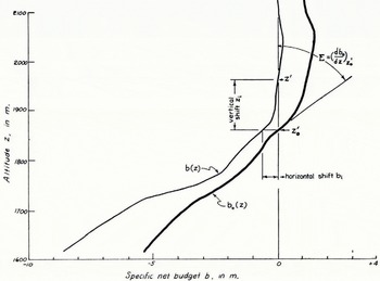
Fig. 2. Vertical variation in specific net budget for South Cascade Glacier, Washington. The curve b0(z) is an equilibrium net budget curve based on the average of the budget years 1957–58 to 1960–61. The curve b(z) represents the net budget for the 1960–61 year only; this curve was the most divergent of the four which were averaged to draw b0(z)
If the net budget-altitude function b(z) is known for several different years, and if this function varies in a regular way from year to year, it may be possible to predict b(z) from known values at just one or two points, utilizing an equation similar to equation 15. Crude approximations to the mass budget relations can even be obtained by extrapolating a known b(z) from one glacier to other glaciers in the immediate area. In some cases b(z) approximates an analytical function such as a parabola (Reference FinsterwalderFinsterwalder, 1954, p. 309) or a straight line (Reference LliboutryLliboutry, 1955, p. 510), but in most cases will be an irregular curve (Fig. 2).
The shape of the b(z) function often is relatively constant from year to year, but the curves are generally displaced from a steady-state value b 0(z). If budget values are plotted horizontally and altitude is plotted vertically on graph paper, one can define either a vertical shift or a horizontal shift in the budget-altitude curves. The former case implies that b(z)=b 0(z+z i ), whereas the latter case implies that b(z)=(b 0+b i )(z). Much actual field data indicates that a horizontal shift is often a better approximation than a vertical shift, as shown in Figure 2. In this case the total net budget can be very simply determined as B=b i S.
The value of budget imbalance is obtained directly by subtracting the steady-state budget value at that altitude from the measured value. In the case of a vertical shift, the steady-state equilibrium line altitude must be subtracted from the observed equilibrium line altitude and the budget imbalance determined using knowledge of the slope of b(z).
The quantity,
Thus the budget imbalance can be determined for any given year from just the altitude of the equilibrium line, if z′0 and E are known.
When b and δS are plotted as simple functions of z, it is difficult to tell from the plot whether the data indicate a steady-state condition or not. For some purposes it is useful to have a graphical representation which indicates directly the condition of the budget. This can be done in two ways: First, instead of plotting b one can plot the product bδS as a function of z (Reference LliboutryLliboutry, 1955, p. 510). However, this requires a fresh calculation for each altitude interval each budget year. As an alternative, one can plot values of b on a graph in which increments on the altitude scale are made proportional to the area increments δS (Reference SchyttSchytt, 1947, p. 109). This method has the advantage that the same plotting scale can be used for different budget years if the glacier’s area-altitude relation is relatively constant from year to year. In either case a steady-state condition is indicated by equal graph areas above and below the equilibrium line, and budget imbalances are proportional to the differences between the two areas.
Ahlmann (Reference Ahlmann1948, p. 55) has suggested that “the balance-sheet of the regime bears a linear relation to the amount of accumulation and ablation at the firn limit”. In the terminology used here, this statement can be expressed as
If this were generally true (Ahlmann’s results show a remarkably good correlation) this would be a very useful method of determining the accumulation and ablation from simple measurements. However, there seems to be no mathematical validity to the relation. Lliboutry (Reference Lliboutry1955, p. 510) presents cogent reasons for the inapplicability of this rule to some actual field results.
What is Firn?
In the older Alpine literature, the term firn (or névé) was used to describe a material that was both older and more dense than snow. The term was also applied to the accumulation area or upper regions of a glacier, but this geographic usage appears to be largely supplemented at the present time by such compound terms as firn basin, firn field, or firn area. It seems appropriate to restrict the term firn to the material itself, but should it be defined on the basis of certain physical properties or on its time relationships?
Definition based purely on physical properties has a logical basis. The firn-ice boundary is generally placed at the point where the densifying material becomes impermeable to water. Benson and Anderson (personal communication from C. S. Benson) have noted that both the rate and mechanism of densification appear to change at a density of about 0.55 g./cm.3, and suggest that the snow-firn boundary be placed here. The exact value of density at the transition depends on several factors. According to older literature, the division between snow and firn is more often placed at a density of 0.4 g./cm.3. In a polar environment the transition from snow to firn may not occur until a number of years have elapsed, according to the Benson-Anderson definition. However, in a temperate-maritime glacier this type of firn may be produced within fairly short time intervals. Layers with density greater than 0.55 g./cm.3 in material less than a year old have been found in every snow pit or core in South Cascade Glacier, including many samples taken well before the end of the accumulation season (Fig. 3). A definition of firn on the basis of density, or other physical properties, would be almost impossible to apply to studies of this temperate-maritime glacier. Furthermore one would have to say that the winter’s accumulation as sampled in April contained so much per cent firn and so much per cent snow, whereas in May it contained different percentages, and so forth, statements that would clearly contradict the original usage of the term firn.

Fig. 3. Density-depth profile obtained 15 May 1960, at location P−1, South Cascade Glacier, Washington
Many workers now define firn as material which has survived one ablation season (or summer season) but has not yet become impermeable to water.Footnote * This mixed definition seems to be most useful in practice. Admittedly, on the Antarctic plateau one usually cannot identify annual layers during the first inspection of a snow pit, and it may be difficult to define a summer or ablation season. However, one cannot determine the exact density by first inspection either. Perhaps it will be necessary to apply different terminologies for studies on high-polar glaciers from those used on subpolar and temperate glaciers. If the term firn is to be retained, it should be usable for temperate glaciers because of precedent. The term “old snow” seems inappropriate for this usage; if this term were adopted one would have to refer to snow up to one year old as “new snow”.
It is suggested here that firn be defined as material (snow, rime, hoar, refrozen melt water) which has survived to the end of one ablation season and which has not yet compacted and recrystallized to the point where it is impermeable to liquid water. Adoption of this definition will result in a term which can be immediately applied in most field studies, serves a useful purpose in mass balance studies, and avoids the complication of having a vertical section containing alternating layers of different materials (firn and snow). Admittedly, there are theoretical and practical disadvantages to this usage of the word firn. The problem urgently needs discussion and deliberation because of the wide usage of this word by glaciologists and others the world over.
Acknowledgements
This paper was presented at the Symposium on Mass Balance Studies, Cambridge, England, 6 January 1962, and has been slightly modified subsequently. Advice and criticism by many glaciological colleagues have been most helpful. Critical reviews of the manuscript by E. R. LaChapelle and R. P. Sharp were especially appreciated. However, the conclusions and opinions stated herein are entirely those of the author.
Discussion of Dr. M. F. Meier’s Paper
Dr. J. F. Nye: I wonder whether Dr. Meier really wants to stick to measuring things with respect to the vertical rather than normal to the surface. I can see that the vertical is convenient for measuring off maps, but when doing theory the normal to the surface is usually what you want.
Dr. Meier: This is purely an expedient for convenience.
Dr. Nye: Whose convenience?
Dr. Meier: The convenience of the person who has to determine the volumes of mass budget quantities. If we measure in a vertical direction we have no problem, we set all our stakes vertical and then, when we reduce our data, we can plot all these data on a map and draw lines of equal accumulation or ablation, we can then measure the area between these lines and get volumes. If you measure or report your data in terms of normals there is no easy way these data can be reduced.
Mr. G. Seligman: If you had a very steep glacier, as opposed to a fairly flat one, would not your values be entirely different?
Dr. Meier: No, I think not.
Dr. J. W. Glen: Can you reasonably define the area of a glacier for the purpose of your integrations to get total budget quantities? Is it the minimum area the glacier has in a budget year?
Dr. Meier: I personally have had to relate glacier quantities to hydrologic quantities which include the whole drainage basin, and this is a very formidable problem when it comes to actual field data. There are two ways to handle this problem; one is to define a glacier area which is only part of a drainage basin on the basis, as you say, of the minimum glacier area during a budget year or the glacier area at the end of a budget year defined on this basis for the whole basin, the other way is to assume that all the area which is ice- or snow-covered is glacier, and this means that the area is a function of time and one must then integrate with respect to time during a budget year. I have found that from a practical point of view the second approach, the time differential is a little easier. P. Kasser reports the other; he defines a specific glacier area and a specific marginal area which is non-glacierized. The difficulty here of course is that there is a constant transfer by avalanches, especially in the Alpine glaciers, from one area to the other.
Dr. H. Lister: The very practical difficulties of measuring quantities at a point are surely such that your algebra ceases to be very applicable when you start dealing with a large ice cap or an ice sheet, since you cannot really take very many measurements for the ablation and accumulation during one year. Is what you have suggested not applicable only to the rather more Iimited size of glacier?
Dr. Meier: I do not know what more one can do, even on ice sheets. When one tries to apply it to the actual field data, then of course there are compromises and approximations that must enter in; these will be different for ice sheets and for small glaciers, but when you have only few data over a large area, the problems are extreme.
Dr. W. H. Ward: Your equilibrium line is a vertical surface through the glacier; this seems an arbitrary result.
Dr. Meier: Yes, it may correspond to absolutely nothing in the glacier itself; the firn line you can see, and it may well be that in many glaciers you can use the terms firn line and equilibrium line interchangeably; in some I know we cannot.
Mr. J. Macdowall: In looking at the ablation on ice sheets, one of the difficulties in applying this is going to be the time scale you use for your observations. People are particularly interested in the ablation, and if you measure this at daily intervals you will get quite different answers from what you would get if you measured it monthly. Your
Dr. Meier: They should be instantaneous values, measured every second! This is a very real problem.
Dr. Glen: Is it not a worse problem even than measuring it every second? In cases where you have wind, you have to decide where the surface of your glacier is.
Dr. Meier: Yes, that is right.
Dr. G. de Q. Robin (Chairman): I think I should now thank Dr. Meier very much for putting some system into our study of mass budgets. There are two points I would like to see myself; first, apart from the rigorous mathematical definitions, I would like to see the various quantities defined in a way which gives non-mathematicians a good appreciation of what is implied, and secondly I think we might manage to simplify some of the terms—cumulative mass flux and things like that do not trip off the tongue frightfully easily for a non-mathematician. Perhaps with discussion and correspondence we may get some slightly less complex terms; but this is no real criticism at all, it is extremely valuable to have had some precision in our thinking on these problems, and I would like to thank Dr. Meier for this contribution.


