


1. Introduction
The aim of this article is to show how time series modelsFootnote 1 can be used to track the progress of an epidemic, forecast key variables and evaluate the effects of policies. Developing effective techniques to accomplish these tasks is of some importance, because, as documented by Ioannidis et al. (Reference Ioannidis, Cripps and Tanner2020), the performance of many of the methods used to forecast the current COVID-19 epidemic has not been impressive. The new models draw much of their inspiration from time series econometrics. However, the characteristics of time series for epidemics are different from those of most time series in economics and these differences need to be taken into account.
Harvey and Kattuman (Reference Harvey and Kattuman2020)—hereafter HK—developed a class of univariate time series models for predicting future values of a variable which when cumulated is subject to an unknown saturation level. In these models, the logarithm of the growth rate of the cumulated series dependsFootnote
2 on a time trend. Allowing this trend to be time-varying introduces flexibility which, in the context of an epidemic, enables the effects of changes in policy and population behaviour to be tracked. Nowcasts and forecasts of the variables of interest, such as the daily number of cases, its growth rate and the instantaneous reproduction number, $ {R}_t, $
can be made. Estimation of the models is by maximum likelihood (ML) and goodness of fit can be assessed by standard statistical test procedures.
$ {R}_t, $
can be made. Estimation of the models is by maximum likelihood (ML) and goodness of fit can be assessed by standard statistical test procedures.
Time series models can also be used to address other questions by exploring relationships between different series. One application concerns how the time path of an epidemic in a country which suffers an outbreak before another can be used as a leading indicator. The rationale for modelling the logarithm of the growth rate (of the cumulated series) comes from the properties of a Gompertz growth curve and when two such curves follow the same time path, but one lags the other, the trends in the series on the logarithms of the growth rate are a constant distance apart. This suggests that when the trends are stochastic, the same will be true. This situation, known as a balanced growth, arises in macroeconomics and is a special case of what econometricians call co-integration; see, for example, Stock and Watson (Reference Stock and Watson1988). The situation is illustrated by showing how the time path of deaths in the UK in the first few months of the coronavirus epidemic follows the time path of deaths in Italy 2 weeks earlier.
The requirement that two series exhibit balanced growth, while highly desirable, is not necessary for one to be a good leading indicator of the other. The need for additional flexibility is explored with data from the ‘second wave’ of coronavirus in Florida in the early part of the summer of 2020 where it is shown how daily new cases can potentially offer improved forecasts of deaths in 2–3 weeks’ time. The forecasts are based on a bivariate unobserved component time series model that combines the dynamic information in the two series by a common trend specified as an integrated random walk (IRW) but includes an independent random walk (RW) component for new cases.
Time series modelling of an intervention can be used to assess the impact of a policy. This was done in HK in connection with the UK lockdown of March 2020. Here, an attempt is made to answer the question ‘What if lockdown had been imposed a week earlier?’ The impact of lockdowns is explored further by developing the ideas associated with balanced growth to try to estimate the number of coronavirus deaths in Sweden had a more stringent lockdown been imposed. The methodology draws on the study of control groups in time series by Harvey and Thiele (Reference Harvey and Thiele2021). It is argued that the fact that death rates in Sweden were roughly 10 times those in neighbouring countries could be misleading; the growth paths of the UK and Italy provide more relevant information. A comparison is made with studies based on the synthetic control (SC) method of Abadie et al. (Reference Abadie, Diamond and Hainmueller2010, Reference Abadie, Diamond and Hainmueller2015).
2. Growth curves and time series models
This section sets out the basic model in which the logarithm of the growth rate of the cumulated series consists of a stochastic trend plus an irregular term. It is then shown how the framework may be extended to model the relationship between two series.
2.1. Dynamic trend models
The observational model uses data on the time series of the cumulated total of confirmed cases or deaths, $ {Y}_t, $ $ t=0,1,\dots, T, $
and the daily change,
$ t=0,1,\dots, T, $
and the daily change, $ {y}_t=\Delta {Y}_t={Y}_t-{Y}_{t-1}. $
HK show how the theory of generalised logistic growth curves suggests models for
$ {y}_t=\Delta {Y}_t={Y}_t-{Y}_{t-1}. $
HK show how the theory of generalised logistic growth curves suggests models for $ \ln \kern0.5em {y}_t $
and
$ \ln \kern0.5em {y}_t $
and $ \ln \kern0.5em {g}_t $
, where
$ \ln \kern0.5em {g}_t $
, where $ {g}_t={y}_t/{Y}_{t-1} $
or
$ {g}_t={y}_t/{Y}_{t-1} $
or $ \Delta \ln \kern0.5em {Y}_t. $
For the special case of the Gompertz growth curve:
$ \Delta \ln \kern0.5em {Y}_t. $
For the special case of the Gompertz growth curve:
 $$ \ln \kern0.5em {y}_t=\ln \kern0.5em {Y}_{t-1}+\delta -\gamma t+{\varepsilon}_t,\kern0.5em \gamma >0,\kern1em t=1,\dots, T, $$
and
 $$ \ln \kern0.5em {g}_t=\delta -\gamma t+{\varepsilon}_t,\kern1em t=1,\dots, T, $$
where $ {\varepsilon}_t $
is a random disturbance term.
$ {\varepsilon}_t $
is a random disturbance term.
A stochastic, or time-varying, trend may be introduced into (2), to give the dynamic trend model:
 $$ \ln \kern0.5em {g}_t={\delta}_t+{\varepsilon}_t,\kern1em {\varepsilon}_t\sim NID\left(0,{\sigma}_{\varepsilon}^2\right),\kern2em t=1,\dots, T, $$
where
 $$ {\displaystyle \begin{array}{lllll}{\delta}_t& =& {\delta}_{t-1}-{\gamma}_{t-1}+{\eta}_t,& \kern1em & {\eta}_t\sim NID\left(0,{\sigma}_{\eta}^2\right),\\ {}{\gamma}_t& =& {\gamma}_{t-1}+{\zeta}_t,& \kern1em & {\zeta}_t\sim NID\left(0,{\sigma}_{\zeta}^2\right),\end{array}} $$
and the normally distributed irregular, level and slope disturbances, $ {\varepsilon}_t, $ $ {\eta}_t $
and
$ {\eta}_t $
and $ {\zeta}_t $
, respectively, are mutually independent. When
$ {\zeta}_t $
, respectively, are mutually independent. When $ {\sigma}_{\zeta}^2 $
is positive, but
$ {\sigma}_{\zeta}^2 $
is positive, but $ {\sigma}_{\eta}^2=0, $
the trend is an IRW. HK found an IRW trend to be particularly useful for tracking an epidemic and it will be adopted in the applications here. The speed with which a trend adapts to a change depends on the signal-noise ratio, which for the IRW is
$ {\sigma}_{\eta}^2=0, $
the trend is an IRW. HK found an IRW trend to be particularly useful for tracking an epidemic and it will be adopted in the applications here. The speed with which a trend adapts to a change depends on the signal-noise ratio, which for the IRW is $ {q}_{\zeta }={\sigma}_{\zeta}^2/{\sigma}_{\varepsilon}^2; $
when
$ {q}_{\zeta }={\sigma}_{\zeta}^2/{\sigma}_{\varepsilon}^2; $
when $ {q}_{\zeta }=0 $
the trend is deterministic, as in (2).
$ {q}_{\zeta }=0 $
the trend is deterministic, as in (2).
Allowing $ {\gamma}_t $
to change over time means that the progress of the epidemic is no longer tied to the proportion of the population infected as it would be if
$ {\gamma}_t $
to change over time means that the progress of the epidemic is no longer tied to the proportion of the population infected as it would be if $ {Y}_t $
followed a deterministic growth curve. Instead the model adapts to movements brought about by changes in behaviour and policies. If
$ {Y}_t $
followed a deterministic growth curve. Instead the model adapts to movements brought about by changes in behaviour and policies. If $ {\gamma}_t $
falls to zero, the growth in
$ {\gamma}_t $
falls to zero, the growth in $ {Y}_t $
becomes exponential while a negative
$ {Y}_t $
becomes exponential while a negative $ {\gamma}_t $
means that the growth rate is increasing. This flexibility also allows the model to deal with second waves, where infections start to increase sharply after having fallen to a relatively low level. The Florida exampleFootnote
3 of Section 4.2 shows how the model deals successfully with a second wave and Harvey et al. (Reference Harvey and Kattuman2021) report accurate forecast for the second UK wave of early 2021. A modification of the model, that is currently under investigation, is to re-initialize the cumulative total at the low point before a new wave begins. The way in which the cumulative total enters the model is important because a key feature of the dynamic Gompertz model is its ability to detect upcoming turning points and to make forecasts that show a downward movement even before a peak has been reached; see, for example, the forecasts made for Germany in HK.
$ {\gamma}_t $
means that the growth rate is increasing. This flexibility also allows the model to deal with second waves, where infections start to increase sharply after having fallen to a relatively low level. The Florida exampleFootnote
3 of Section 4.2 shows how the model deals successfully with a second wave and Harvey et al. (Reference Harvey and Kattuman2021) report accurate forecast for the second UK wave of early 2021. A modification of the model, that is currently under investigation, is to re-initialize the cumulative total at the low point before a new wave begins. The way in which the cumulative total enters the model is important because a key feature of the dynamic Gompertz model is its ability to detect upcoming turning points and to make forecasts that show a downward movement even before a peak has been reached; see, for example, the forecasts made for Germany in HK.
Additional components, such as day of the week effects, can be added to (3). These may be deterministic or stochastic. Explanatory variables, including interventions, can also be included, as may stationary components. Thus (3) could become:
 $$ \ln \kern0.5em {g}_t={\delta}_t+{\theta}_t+{\mu}_t+{\mathbf{x}}_t^{\prime}\boldsymbol{\beta} +{\varepsilon}_t,\kern2em t=1,\dots, T, $$
where $ {\theta}_t $
is a stochastic daily component, modelled as in Harvey (Reference Harvey1989, pp. 43–4),
$ {\theta}_t $
is a stochastic daily component, modelled as in Harvey (Reference Harvey1989, pp. 43–4), $ {\mu}_t $
is a stationary autoregressive process,
$ {\mu}_t $
is a stationary autoregressive process, $ {\mathbf{x}}_t $
is a vector of explanatory variables and
$ {\mathbf{x}}_t $
is a vector of explanatory variables and $ \boldsymbol{\beta} $
is a corresponding vector of parameters. Possible candidates for explanatory variables include stringency indices for governmental policies, as in Hale et al. (Reference Hale, Angrist, Goldszmidt, Kira, Petherick, Phillips, Webster, Cameron-Blake, Hallas, Majumdar and Tatlow2021). All these models can be handled using techniques based on state space models and the Kalman filter (KF); see Durbin and Koopman (Reference Durbin and Koopman2012). Here, the STAMP package of Koopman et al. (Reference Koopman, Lit and Harvey2021) is used. Estimation of the unknown parameters is by ML. Diagnostic tests for normality and residual serial correlation are based on the one-step ahead prediction errors,
$ \boldsymbol{\beta} $
is a corresponding vector of parameters. Possible candidates for explanatory variables include stringency indices for governmental policies, as in Hale et al. (Reference Hale, Angrist, Goldszmidt, Kira, Petherick, Phillips, Webster, Cameron-Blake, Hallas, Majumdar and Tatlow2021). All these models can be handled using techniques based on state space models and the Kalman filter (KF); see Durbin and Koopman (Reference Durbin and Koopman2012). Here, the STAMP package of Koopman et al. (Reference Koopman, Lit and Harvey2021) is used. Estimation of the unknown parameters is by ML. Diagnostic tests for normality and residual serial correlation are based on the one-step ahead prediction errors, $ {v}_t=\ln \kern0.5em {g}_t-{\delta}_{t|t-1},t=3,\dots, T. $
The KF outputs the estimates and forecasts of the state vector $ {\left({\delta}_t,{\gamma}_t\right)}^{\prime }. $
Estimates at time
$ {\left({\delta}_t,{\gamma}_t\right)}^{\prime }. $
Estimates at time $ t $
conditional on information up to and including time
$ t $
conditional on information up to and including time $ t $
are denoted
$ t $
are denoted $ {\left({\delta}_{t|t},{\gamma}_{t|t}\right)}^{\prime } $
, while predictions
$ {\left({\delta}_{t|t},{\gamma}_{t|t}\right)}^{\prime } $
, while predictions $ j $
steps ahead are
$ j $
steps ahead are $ {\left({\delta}_{t+j|t},{\gamma}_{t+j|t}\right)}^{\prime }. $
The smoother, which estimates the state at time
$ {\left({\delta}_{t+j|t},{\gamma}_{t+j|t}\right)}^{\prime }. $
The smoother, which estimates the state at time $ t $
based on all
$ t $
based on all $ T $
observations in the series, is denoted
$ T $
observations in the series, is denoted $ {\left({\delta}_{t|T},{\gamma}_{t|T}\right)}^{\prime } $
.
$ {\left({\delta}_{t|T},{\gamma}_{t|T}\right)}^{\prime } $
.
Remark 1. When the observations are small, a negative binomial distribution for $ {y}_t, $
conditional on past observations, may be appropriate. HK show how the model may be modified to deal with this possibility. However, the numbers in the applications here are big enough to allow
$ {y}_t, $
conditional on past observations, may be appropriate. HK show how the model may be modified to deal with this possibility. However, the numbers in the applications here are big enough to allow $ {y}_t $
to be treated as conditionally lognormal and hence for the conditional distribution of
$ {y}_t $
to be treated as conditionally lognormal and hence for the conditional distribution of $ \ln \kern0.5em {g}_t $
to be considered normal.
$ \ln \kern0.5em {g}_t $
to be considered normal.
2.2. Forecasts
The forecasts of the trend in future values of $ \ln \kern0.5em {g}_t $
in the dynamic Gompertz model are given by
$ \ln \kern0.5em {g}_t $
in the dynamic Gompertz model are given by $ {\delta}_{T+\mathrm{\ell}\mid T}={\delta}_{T\mid T}-{\gamma}_{T\mid T}\mathrm{\ell}, $ $ \mathrm{\ell}=1,2,\dots, $
where
$ \mathrm{\ell}=1,2,\dots, $
where $ {\delta}_{T\mid T} $
and
$ {\delta}_{T\mid T} $
and $ {\gamma}_{T\mid T} $
are the KF estimates of
$ {\gamma}_{T\mid T} $
are the KF estimates of $ {\delta}_T $
and
$ {\delta}_T $
and $ {\gamma}_T $
at the end of the sample. Forecasts of the trend in the daily observations are obtained from a recursion for the trend in their cumulative total,
$ {\gamma}_T $
at the end of the sample. Forecasts of the trend in the daily observations are obtained from a recursion for the trend in their cumulative total, $ {Y}_t $
, namely,
$ {Y}_t $
, namely,
 $$ {\mu}_{T+\mathrm{\ell}\mid T}={\mu}_{T+\mathrm{\ell}-1\mid T}\left(1+{g}_{T+\mathrm{\ell}\mid T}\right),\kern2em \mathrm{\ell}=1,2,\dots, \kern1em $$
where $ {g}_{T+\mathrm{\ell}\mid T}=\exp {\delta}_{T+\mathrm{\ell}\mid T} $
and
$ {g}_{T+\mathrm{\ell}\mid T}=\exp {\delta}_{T+\mathrm{\ell}\mid T} $
and $ {\mu}_{T\mid T}={Y}_T $
. The trend in the daily figures is then,
$ {\mu}_{T\mid T}={Y}_T $
. The trend in the daily figures is then,
 $$ {\mu}_{y,T+\mathrm{\ell}\mid T}={g}_{T+\mathrm{\ell}\mid T}{\mu}_{T+\mathrm{\ell}-1\mid T}\kern0.5em ,\kern2em \mathrm{\ell}=1,2,\dots $$
Daily effects can be added to $ {\delta}_t. $
In this case, forecasts of the observations themselves, that is
$ {\delta}_t. $
In this case, forecasts of the observations themselves, that is $ {\hat{y}}_{T+\mathrm{\ell}\mid T} $
and
$ {\hat{y}}_{T+\mathrm{\ell}\mid T} $
and $ {\hat{Y}}_{T+\mathrm{\ell}\mid T}, $
are given by adding the filtered value of the daily component to the trend component,
$ {\hat{Y}}_{T+\mathrm{\ell}\mid T}, $
are given by adding the filtered value of the daily component to the trend component, $ {\delta}_{T+\mathrm{\ell}\mid T} $
.
$ {\delta}_{T+\mathrm{\ell}\mid T} $
.
Unlike most other forecasting methods, the dynamic Gompertz model yields prediction intervals. The way in which they are constructed is set out in Section 2.4 of Harvey et al. (Reference Harvey, Kattuman and Thamotheram2021) and examples are given.
2.3. Forecasting and nowcasting R
Harvey and Kattuman (Reference Harvey and Kattuman2021) use filtered estimates of $ {g}_{y,t}, $
given by
$ {g}_{y,t}, $
given by $ {g}_{y,t\mid t}={g}_{t\mid t}-{\gamma}_{t\mid t}, $
to track the progress of an epidemic. A corresponding estimator of the instantaneous reproduction number,
$ {g}_{y,t\mid t}={g}_{t\mid t}-{\gamma}_{t\mid t}, $
to track the progress of an epidemic. A corresponding estimator of the instantaneous reproduction number, $ {R}_t, $
can be constructed in a number of ways, as in Wallinga and Lipsitch (Reference Wallinga and Lipsitch2007). The most practical for COVID-19 are:
$ {R}_t, $
can be constructed in a number of ways, as in Wallinga and Lipsitch (Reference Wallinga and Lipsitch2007). The most practical for COVID-19 are:
 $$ {\tilde{R}}_{t,\tau }=1+\tau {g}_{y,t\mid t}\kern1.5em \mathrm{and}\kern1em {\tilde{R}}_{t,\tau}^e=\exp \left(\tau {g}_{y,t\mid t}\right), $$
where $ \tau $
is the generation interval, which is the number of days that must elapse before an infected person can transmit the disease; setting
$ \tau $
is the generation interval, which is the number of days that must elapse before an infected person can transmit the disease; setting $ \tau =4 $
is a good choice. Harvey and Kattuman (Reference Harvey and Kattuman2021) provide more details and show how forecasts of
$ \tau =4 $
is a good choice. Harvey and Kattuman (Reference Harvey and Kattuman2021) provide more details and show how forecasts of $ {R}_{t,\tau } $
, with associated prediction intervals. Harvey et al. (Reference Harvey, Kattuman and Thamotheram2021) illustrate the implementation of this approach in the NIESR tracker.
$ {R}_{t,\tau } $
, with associated prediction intervals. Harvey et al. (Reference Harvey, Kattuman and Thamotheram2021) illustrate the implementation of this approach in the NIESR tracker.
2.4. Panel data
The extended dynamic Gompertz model of (5) can be used as the basis for handling panel data. When there are $ N $
cross-sectional units,
$ N $
cross-sectional units,
 $$ \ln \kern0.5em {g}_{it}={\delta}_{it}+{\mathbf{z}}_{it}^{\prime }{\boldsymbol{\alpha}}_i+{\mathbf{x}}_{it}^{\prime}\boldsymbol{\beta} +{\varepsilon}_{it},\kern1.5em i=1,\dots, N,\kern1.5em t=1,\dots, T, $$
where $ {\delta}_{it}^{\prime }s $
are stochastic trend components and
$ {\delta}_{it}^{\prime }s $
are stochastic trend components and $ {\mathbf{z}}_{it} $
and
$ {\mathbf{z}}_{it} $
and $ {\mathbf{x}}_{it} $
are vectors of explanatory variables, with
$ {\mathbf{x}}_{it} $
are vectors of explanatory variables, with $ {\boldsymbol{\alpha}}_i, $ $ i=1,\dots, N, $
and
$ i=1,\dots, N, $
and $ \boldsymbol{\beta} $
denoting associated coefficients. It may be necessary to add autoregressive and day of the week components. Either way, we can pre-filter with the univariate filter, as in Harvey (Reference Harvey1989, Sect. 3.4.2) and then, if the components are assumed to be mutually independent, use the transformed observation to estimate a standard panel data model. This procedure can be iterated to convergence.
$ \boldsymbol{\beta} $
denoting associated coefficients. It may be necessary to add autoregressive and day of the week components. Either way, we can pre-filter with the univariate filter, as in Harvey (Reference Harvey1989, Sect. 3.4.2) and then, if the components are assumed to be mutually independent, use the transformed observation to estimate a standard panel data model. This procedure can be iterated to convergence.
Further generalisations would let the stochastic trends depend on common factors.
3. Comparing different growth curves
The Gompertz growth curve lies behind the notion of setting up time series models in which the logarithm of the growth rate of the cumulative total of a variable follows a trend. It is therefore able to provide insight on how to formulate and interpret models linking several series.
The Gompertz growth curve is:
 $$ \mu (t)=\overline{\mu}\exp \left(-\alpha {e}^{-\gamma t}\right),\kern2em \alpha, \gamma >0,\kern2em -\infty <t<\infty, $$
where $ \gamma $
is a growth rate parameter,
$ \gamma $
is a growth rate parameter, $ \overline{\mu} $
is the upper bound or saturation level (
$ \overline{\mu} $
is the upper bound or saturation level ( $ \mu (t)\kern1.em \to \kern1.5em \overline{\mu} $
as
$ \mu (t)\kern1.em \to \kern1.5em \overline{\mu} $
as $ t\to \infty \Big) $
and
$ t\to \infty \Big) $
and $ \alpha $
reflects initial conditions. The associated incidence curve is:
$ \alpha $
reflects initial conditions. The associated incidence curve is:
 $$ d\mu (t)/ dt={\mu}^{\prime }(t)=\gamma \alpha \mu (t)\exp \left(-\gamma t\right), $$
with a peak at $ t={\gamma}^{-1}\ln \kern0.5em \alpha . $
Figure 1 shows an incidence curve with a peak at
$ t={\gamma}^{-1}\ln \kern0.5em \alpha . $
Figure 1 shows an incidence curve with a peak at $ t=19.97 $
, together with the same curve shifted to the right so the peak is at
$ t=19.97 $
, together with the same curve shifted to the right so the peak is at $ 30.71. $
A curve above the right hand curve is also shown; this is higher because the value of
$ 30.71. $
A curve above the right hand curve is also shown; this is higher because the value of $ \overline{\mu} $
is 1400 rather than 1000 as it is for the other two curves. In all cases
$ \overline{\mu} $
is 1400 rather than 1000 as it is for the other two curves. In all cases $ \gamma =0.15, $
but for the left hand curve
$ \gamma =0.15, $
but for the left hand curve $ \alpha $
is 20 whereas for the right hand curves it is 100.
$ \alpha $
is 20 whereas for the right hand curves it is 100.
(Colour online) Gompertz incidence curves, $ {\mu}^{\prime }(t), $
with
$ {\mu}^{\prime }(t), $
with $ \gamma =0.15, $ $ {\alpha}_1=20 $
for the left hand curve and
$ {\alpha}_1=20 $
for the left hand curve and $ {\alpha}_2=100 $
for the right hand curves; the value of
$ {\alpha}_2=100 $
for the right hand curves; the value of $ \overline{\mu} $
in the upper curve is 1400 as opposed to 1000 as in the lower curve
$ \overline{\mu} $
in the upper curve is 1400 as opposed to 1000 as in the lower curve

Although the right hand curves in figure 1 clearly lag the left hand one, it is not immediately evident how to model the relationship. However, the logarithms of the growth rates of $ \mu (t) $
are:
$ \mu (t) $
are:
 $$ \ln \kern0.5em g(t)=\delta -\gamma t,\kern2em t\kern0.5em \ge \kern0.5em 0, $$
where $ \delta = $ $ \ln \kern0.5em \alpha \gamma; $
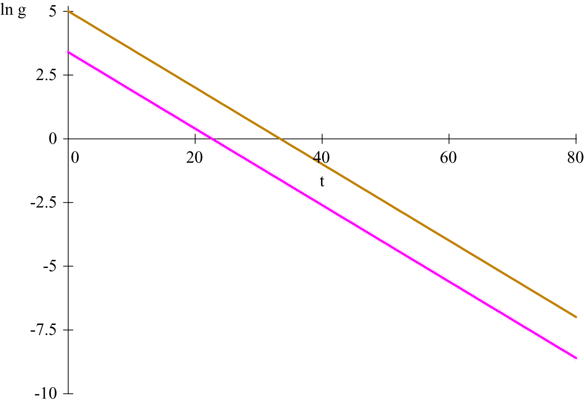
compare (2). Figure 2 shows the two lines for
$ \ln \kern0.5em \alpha \gamma; $
compare (2). Figure 2 shows the two lines for $ \ln \kern0.5em g(t) $
running in parallel. The distance between them depends on the intercepts,
$ \ln \kern0.5em g(t) $
running in parallel. The distance between them depends on the intercepts, $ \delta, $
which in turn depend on the initialization parameter,
$ \delta, $
which in turn depend on the initialization parameter, $ \alpha . $
The height of the incidence curve, which depends on the saturation level,
$ \alpha . $
The height of the incidence curve, which depends on the saturation level, $ \overline{\mu}, $
is irrelevant; as a result, the lines corresponding to the two right-hand incidence curves in figure 1 are identical. This is important because it means that small populations can be compared with big ones: size does not matter.
$ \overline{\mu}, $
is irrelevant; as a result, the lines corresponding to the two right-hand incidence curves in figure 1 are identical. This is important because it means that small populations can be compared with big ones: size does not matter.
(Colour online) Logarithms of the growth rates for incidence curves in figure 1; $ \gamma =0.15, $ $ {\alpha}_1=20 $
and
$ {\alpha}_1=20 $
and $ {\alpha}_2=100 $
(upper line)
$ {\alpha}_2=100 $
(upper line)
When two lines are parallel, the upper line lags the lower one by:
 $$ k=\frac{\delta_2-{\delta}_1}{\gamma }=\frac{\ln \kern0.5em {\alpha}_2-\ln \kern0.5em {\alpha}_1}{\gamma }, $$
where $ {\delta}_1 $
and
$ {\delta}_1 $
and $ {\delta}_2 $
are the intercepts of the lower and upper lines, respectively and
$ {\delta}_2 $
are the intercepts of the lower and upper lines, respectively and $ {\alpha}_1 $
and
$ {\alpha}_1 $
and $ {\alpha}_2 $
are the corresponding initial conditions. In figure 2, the lag is
$ {\alpha}_2 $
are the corresponding initial conditions. In figure 2, the lag is $ k=10.73. $
When the
$ k=10.73. $
When the $ {\gamma}^{\prime }s $
are different, the epidemic progresses at different speeds. The lines for
$ {\gamma}^{\prime }s $
are different, the epidemic progresses at different speeds. The lines for $ \ln \kern0.5em g(t) $
are no longer parallel and the time lag is no longer constant.
$ \ln \kern0.5em g(t) $
are no longer parallel and the time lag is no longer constant.
4. A statistical model for leading indicators
Now consider observational models of the form (2) for two time series which are on the same growth path because $ {\gamma}_1={\gamma}_2 $
but the first series leads the second by
$ {\gamma}_1={\gamma}_2 $
but the first series leads the second by $ k $
time periods. The observations run from
$ k $
time periods. The observations run from $ t=1 $
to
$ t=1 $
to $ T $
but when the first series is lagged by
$ T $
but when the first series is lagged by $ k $
time periods,
$ k $
time periods, $ \ln \kern0.5em {g}_{1,t-k} $
runs from
$ \ln \kern0.5em {g}_{1,t-k} $
runs from $ t=k+1 $
to
$ t=k+1 $
to $ T+k. $
Subtracting the first series from the second gives:
$ T+k. $
Subtracting the first series from the second gives:
 $$ \ln \kern0.5em {g}_{2t}=\delta +\ln \kern0.5em {g}_{1,t-k}+{\varepsilon}_t,\kern0.5em $$
where $ \delta =\ln \kern0.5em \left({\alpha}_2/{\alpha}_1\right) $
and the disturbance term is
$ \delta =\ln \kern0.5em \left({\alpha}_2/{\alpha}_1\right) $
and the disturbance term is $ {\varepsilon}_t={\varepsilon}_{2t}-{\varepsilon}_{1,t-k} $
. The equation takes the same form when the trends are stochastic, so long as there is balanced growth. The disturbance,
$ {\varepsilon}_t={\varepsilon}_{2t}-{\varepsilon}_{1,t-k} $
. The equation takes the same form when the trends are stochastic, so long as there is balanced growth. The disturbance, $ {\varepsilon}_t, $
can replaced by any stationary process.
$ {\varepsilon}_t, $
can replaced by any stationary process.
When the two series are not on the same growth path, there is no longer a value of $ k $
for the contrast in (13) that makes it stationary. The stationarity test of Kwiatkowski et al. (Reference Kwiatkowski, Phillips, Schmidt and Shin1992)—the KPSS test—can be used to test for this possibility.
$ k $
for the contrast in (13) that makes it stationary. The stationarity test of Kwiatkowski et al. (Reference Kwiatkowski, Phillips, Schmidt and Shin1992)—the KPSS test—can be used to test for this possibility.
A bivariate time series model combines the dynamic information in the target series with that in the leading indicator. It is set up by lagging the observations on the leading indicator so that they are aligned with the target. Hence, defining $ {g}_{1,t}^{(k)}={g}_{1,t-k} $
for
$ {g}_{1,t}^{(k)}={g}_{1,t-k} $
for $ t=k+1,..,T+k $
gives:
$ t=k+1,..,T+k $
gives:
 $$ {\displaystyle \begin{array}{l}\ln \kern0.5em {g}_{1,t}^{(k)}={\delta}_t+{\psi}_t+{\varepsilon}_{1t},\kern1.5em t=k+1,.\dots, T+k,\\ {}\ln \kern0.5em {g}_{2t}=\overline{\delta}+{\delta}_t+{\varepsilon}_{2t},\kern5.5em t=k+1,.\dots, T.\end{array}} $$
The $ k $
future values of
$ k $
future values of $ \ln \kern0.5em {g}_{2,T+j}, $ $ j=1,..,k $
are treated as missing observations.Footnote
4 The trend,
$ j=1,..,k $
are treated as missing observations.Footnote
4 The trend, $ {\delta}_t, $
is an IRW that is designed to capture the growth path of the target series. Its initial level has been (arbitrarily) assigned to the first series; hence the need for a constant term,
$ {\delta}_t, $
is an IRW that is designed to capture the growth path of the target series. Its initial level has been (arbitrarily) assigned to the first series; hence the need for a constant term, $ \overline{\delta}, $
in the second. The role of the other stochastic component,
$ \overline{\delta}, $
in the second. The role of the other stochastic component, $ {\psi}_t, $
is to allow for deviations of the leading indicator from the balanced growth path. A convenient specification for it is the first-order autoregressive process,
$ {\psi}_t, $
is to allow for deviations of the leading indicator from the balanced growth path. A convenient specification for it is the first-order autoregressive process,
 $$ {\psi}_t={\phi \psi}_{t-1}+{\zeta}_t,\kern1em {\zeta}_t\sim NID\left(0,{\sigma}_{\zeta}^2\right),\kern1em t=k+1,.\dots, T+k. $$
All disturbances in (14), including $ {\varepsilon}_{1t} $
and
$ {\varepsilon}_{1t} $
and $ {\varepsilon}_{2t}, $
are Gaussian and assumed to be mutually as well as serially independent. Only a single lag is present. More lags could be included, but the aim is find a viable leading indicator for movements in the trend rather than to estimate a distributed lag for the observations. Estimation is by state space methods. As new observations become available, nowcasts and forecasts are updated by the KF.
$ {\varepsilon}_{2t}, $
are Gaussian and assumed to be mutually as well as serially independent. Only a single lag is present. More lags could be included, but the aim is find a viable leading indicator for movements in the trend rather than to estimate a distributed lag for the observations. Estimation is by state space methods. As new observations become available, nowcasts and forecasts are updated by the KF.
When $ \left|\phi \right|<1 $
, the series are co-integrated with balanced growth. In the absence of balanced growth, the suggestion is to let
$ \left|\phi \right|<1 $
, the series are co-integrated with balanced growth. In the absence of balanced growth, the suggestion is to let $ {\psi}_t $
be a RW, by setting
$ {\psi}_t $
be a RW, by setting $ \phi =1 $
. The value of
$ \phi =1 $
. The value of $ k $
is then based on experimentation and prior information about what might constitute a reasonable lag. The hope is that the RW specification for
$ k $
is then based on experimentation and prior information about what might constitute a reasonable lag. The hope is that the RW specification for $ {\psi}_t $
enables its movements to be separated from those in the IRW trend.
$ {\psi}_t $
enables its movements to be separated from those in the IRW trend.
The filtered estimates, $ {g}_{t\mid t} $
and
$ {g}_{t\mid t} $
and $ {\gamma}_{t\mid t}, $
for the target series give the nowcast of
$ {\gamma}_{t\mid t}, $
for the target series give the nowcast of $ {g}_{y,t} $
at time
$ {g}_{y,t} $
at time $ t=T $
and the forecast at
$ t=T $
and the forecast at $ t=T+k $
. Forecasts can also be made beyond
$ t=T+k $
. Forecasts can also be made beyond $ t=T+k, $
but without the benefit of corresponding values of the leading indicator. The KF and smoother implicitly weights observations in both series in order to compute nowcasts and forecasts for the target.
$ t=T+k, $
but without the benefit of corresponding values of the leading indicator. The KF and smoother implicitly weights observations in both series in order to compute nowcasts and forecasts for the target.
4.1. Italy and the UK
Figure 3 shows the daily deaths in Italy and the UK from 2 March to 20 June 2020; after that the numbers for Italy start to become small. The figures are for when the deaths were recorded rather than when they occurred. Series based on date of death would not have the daily pattern but were difficult to obtain at that time. Data sources are given in Appendix A.
(Colour online) Daily deaths from COVID-19 in Italy and UK in 2020

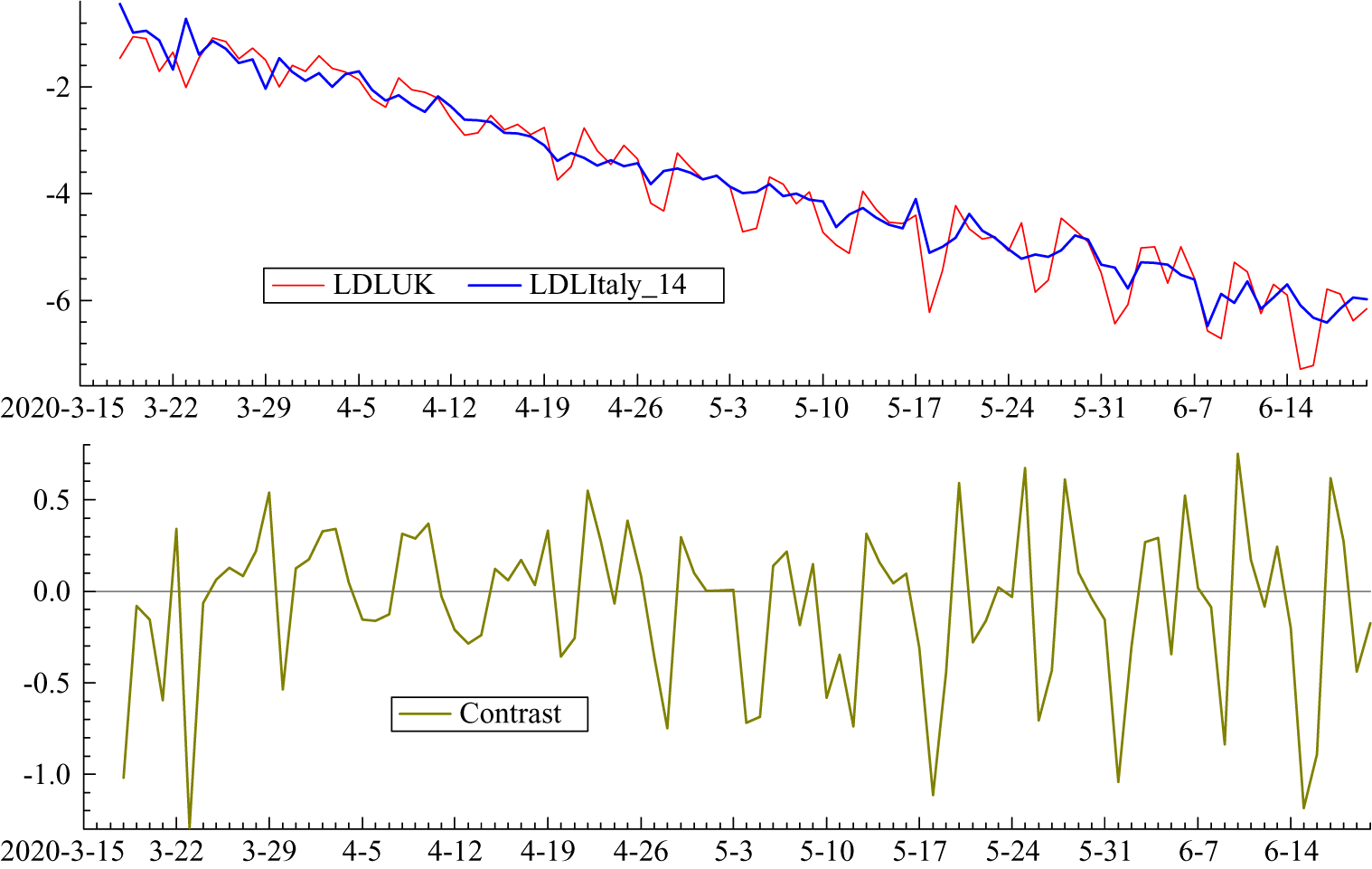
Italy clearly leads the UK but the relationship is captured more precisely in figure 4 which shows the logarithms of the growth rates of total deaths (LDL). The UK numbers are small at the beginning of March and so there are missing observations. A lag of 14 days is not inconsistent with prior information and it has the attraction of lining up the days of the week in the two countries. Other lags were tried but 14 minimised the gap between the two countries. Figure 5 shows the LDL series with Italy lagged by 14 days together with the contrast between the two countries obtained by subtracting Italy from the UK. The contrast series appears to be stationary with a mean close to zero; without the lag for Italy the values at the end of March and the beginning of April tend to be higher than the others, reflecting the later UK lockdown. Estimating a regression model with daily dummy variables removed most of the serial correlation and gave a mean of $ \tilde{\delta}=-0.083, $
with a SE on
$ \tilde{\delta}=-0.083, $
with a SE on $ 0.035. $
The diagnostic statistics wereFootnote
5: r(1) = −0:06;
$ 0.035. $
The diagnostic statistics wereFootnote
5: r(1) = −0:06; $ Q(14)=13.40, $ $ r(1)=-0.06, $ $ BS=1.85 $
and
$ BS=1.85 $
and $ H=1.24. $
(Colour online) Logarithms of the growth rates (LDL) of total deaths in UK and Italy

(Colour online) LDL series from 16 March to 20 June with Italy lagged by 14 days together with the contrast LDLUK–LDLItaly
Fitting a bivariate time series model of the form (14), starting on 16 March and finishing on 5 July, gave a slowly changing trend that was close to being deterministic. The $ {\delta}_{1t} $
term was excluded but a daily component was included. The estimate of the daily growth rate of UK deaths 14 days beyond the final observation on 20 June was
$ {\delta}_{1t} $
term was excluded but a daily component was included. The estimate of the daily growth rate of UK deaths 14 days beyond the final observation on 20 June was $ {g}_{y,T+k\mid T}=-0.058, $
giving a forecast of
$ {g}_{y,T+k\mid T}=-0.058, $
giving a forecast of $ {\tilde{R}}_{T+k,4}=0.77 $
.
$ {\tilde{R}}_{T+k,4}=0.77 $
.
4.2. Deaths and new cases in Florida
Daily cases of COVID-19 in the U.S. state of Florida peaked in early April. There was then a decline following a lockdown during April. After April restrictions were eased and there was a levelling out in May, followed by a sharp rise in June. This second wave poses a challenge for a model in which new cases are used as a leading indicator for deaths. The model deals with the second wave by allowing $ {\gamma}_{t\mid t} $
to become negative; estimates of
$ {\gamma}_{t\mid t} $
to become negative; estimates of $ {R}_t $
can still be obtained from
$ {R}_t $
can still be obtained from $ {g}_{y,t\mid t}, $
as in (8).
$ {g}_{y,t\mid t}, $
as in (8).
Aside from the model having to deal with a situation where new cases and deaths rise and fall, there is the problem that the basis on which new cases are recorded changes over time. At the beginning of the pandemic, new cases in many countries were primarily hospital admissions, but over time testing became more widespread. In the case of Florida, there was an increase in testing in May, although the growth rate in tests was roughly constant from the end of May onwards. This suggests that the growth rate of confirmed new cases may still be a good indicator of the path of new infections; see Harvey and Kattuman (Reference Harvey and Kattuman2021).
The observations, particularly deaths, have a strong weekly pattern. A clearer impression of the underlying trend is given by figure 6 which shows a 7-day moving average of the logarithms of the growth rates of total new cases and deaths from 29 March to 19 July 2020 inclusive. It is apparent that new cases are leading, but the relationship between deaths and new cases is not completely stable over time, partly because of an increase in the growth rate of testing in May and partly because of other factors, such as better hospital treatment. The inclusion of the $ {\psi}_t $
component in model (14) offers a way of dealing with the discrepancy. Nevertheless, despite the instability, it seems clear that new cases peak some time before the end of the sample whereas deaths appear to be at their peak, something confirmed by later observations.
$ {\psi}_t $
component in model (14) offers a way of dealing with the discrepancy. Nevertheless, despite the instability, it seems clear that new cases peak some time before the end of the sample whereas deaths appear to be at their peak, something confirmed by later observations.
(Colour online) Seven-day moving average of LDL deaths in Florida, new cases and new cases lagged 18 days (dotted line) from 29 March till 19 July 2020

The lag in (14) is chosen so as to get maximum benefit for new cases as a leading indicator. It is not trying to model the distribution of days from infection to death although the choice of $ k $
may be roughly aligned with the mean time to death. After some experimentation it was decided to fix the lag at 18. The LDL for new cases shifted in this way, and shown in figure 6, tracks deaths quite well.
$ k $
may be roughly aligned with the mean time to death. After some experimentation it was decided to fix the lag at 18. The LDL for new cases shifted in this way, and shown in figure 6, tracks deaths quite well.
The model, including day of the week variables, was fitted to the Florida data from 29 March till 19 July, with the new cases shifted forward 18 days so as to end on 6 August; thus $ k=18 $
. Specifying
$ k=18 $
. Specifying $ {\psi}_t $
as a first-order autoregressive process in (14) gave an estimated
$ {\psi}_t $
as a first-order autoregressive process in (14) gave an estimated $ \phi $
of 0.998, so a RW seems appropriate. The smoothed estimates of this RW component are shown in figure 7. The lower graph is the smoothed estimates of the day of the week component in deaths; note that the bivariate model is able to give estimates for the period after 19 July when there are no observations on deaths. The size and variability of the daily component in deaths is much bigger than it is for new cases, with the very high variation coinciding with the period when the numbers of deaths are relatively small. Similarly the prediction error variance of 0.115 for new cases was less than half the 0.253 obtained for deaths. Little serial correlation remained in the residuals for deaths: the Box–Ljung Q-statistic for the first 18 residual autocorrelations was 8.16, while the corresponding figure for cases was a little higherFootnote
6 at 25.01. The signal-noise ratio was estimated as 0.00037, so the trend changes relatively slowly but is still able to adapt to changes in direction.
$ \phi $
of 0.998, so a RW seems appropriate. The smoothed estimates of this RW component are shown in figure 7. The lower graph is the smoothed estimates of the day of the week component in deaths; note that the bivariate model is able to give estimates for the period after 19 July when there are no observations on deaths. The size and variability of the daily component in deaths is much bigger than it is for new cases, with the very high variation coinciding with the period when the numbers of deaths are relatively small. Similarly the prediction error variance of 0.115 for new cases was less than half the 0.253 obtained for deaths. Little serial correlation remained in the residuals for deaths: the Box–Ljung Q-statistic for the first 18 residual autocorrelations was 8.16, while the corresponding figure for cases was a little higherFootnote
6 at 25.01. The signal-noise ratio was estimated as 0.00037, so the trend changes relatively slowly but is still able to adapt to changes in direction.
(Colour online) Smoothed estimates of the RW component in Florida new cases, shifted forward by 18 days and the associated daily component in deaths

Figure 8 shows the forecasts of the logarithm of the growth rate deaths, obtained by using the leading indicator, together with the actual observations from 20 July to 4 August. The smooth dotted line is the trend in LDL deaths. As can be seen, the model forsees the turning point. By contrast, the growth rate of LDL deaths on 19 July is still positive, and estimating a univariate model up to this point gave forecasts continuing on an upward path, overshooting the actual observations.
(Colour online) Forecasts (dots) and trend (smooth dots) of the logarithm of the growth rate of deaths, obtained by using the leading indicator, together with the actual observations from 20 July to 4 August; observations before 20 July (LDLFlDeath) shown by thick line

5. Policy interventions and control groups
This section shows how the time series models can be used to assess the effects of policy. The first example uses univariate time series modelling to investigate the timing of the UK lockdown in the spring of 2020. The second illustrates how the balanced growth framework provides the basis for policy evaluation by showing how some variables can be used as control groups for a target variable. The consequences of Sweden’s soft lockdown coronavirus policy in the early part of 2020 are assessed and a comparison is made with studies based on the method of SC.
5.1. What if the March 2020 lockdown in the UK had been a week earlier?
The UK went into full lockdown on 23 March. Can we estimate how many deaths could have been saved if it had been a week earlier?
A slope intervention in (2) enables the effect of a policy which changes $ \gamma $
to be evaluated. Thus,
$ \gamma $
to be evaluated. Thus,
 $$ \ln \kern0.5em {g}_t=\delta -\gamma t-\beta {tw}_t+{\varepsilon}_t,\kern1em t=1,\dots, T, $$
where $ {w}_t $
are intervention dummy variables. When the full effect is realised, the slope on the time trend will have moved from
$ {w}_t $
are intervention dummy variables. When the full effect is realised, the slope on the time trend will have moved from $ \gamma $
to
$ \gamma $
to $ \gamma +\beta . $
A positive
$ \gamma +\beta . $
A positive $ \beta $
lowers the growth rate,
$ \beta $
lowers the growth rate, $ {g}_t, $
the peak of the incidence curve and the final level. The intervention dummies can be constructed from a logistic cumulative distribution function, giving a response curve:
$ {g}_t, $
the peak of the incidence curve and the final level. The intervention dummies can be constructed from a logistic cumulative distribution function, giving a response curve:
 $$ W(t)=1/\Big(1+\exp \left(-\gamma \left(t-{t}^{\mathrm{med}}\right)\right),\kern2em -\infty <W(t)<\infty, $$
where $ {t}^{\mathrm{med}} $
is the median. With
$ {t}^{\mathrm{med}} $
is the median. With $ {t}^L $
and
$ {t}^L $
and $ {t}^U $
denoting the beginning and end of the time span during which the response to the intervention occurs, the dummy variables are defined as
$ {t}^U $
denoting the beginning and end of the time span during which the response to the intervention occurs, the dummy variables are defined as $ {w}_t=0 $
for
$ {w}_t=0 $
for $ t<{t}^L, $ $ {w}_t=W(t) $
for
$ {w}_t=W(t) $
for $ {t}^L, $ $ t= $ $ {t}^L+1,..,{t}^I,..,{t}^U $
and
$ {t}^L+1,..,{t}^I,..,{t}^U $
and $ {w}_t=1 $
for
$ {w}_t=1 $
for $ t={t}^U+1,..,T. $
HK fitted the static model in (15) to new cases in the UK, with an intervention starting on 26 March and ending on 12 April, using data from the beginning of March up to 29 April. The result was an estimate of
$ t={t}^U+1,..,T. $
HK fitted the static model in (15) to new cases in the UK, with an intervention starting on 26 March and ending on 12 April, using data from the beginning of March up to 29 April. The result was an estimate of $ \beta $
equal to
$ \beta $
equal to $ 0.020 $ $ (0.004) $
and an estimate of
$ (0.004) $
and an estimate of $ \gamma $
also equal to
$ \gamma $
also equal to $ 0.020. $
The overall effectFootnote
7 is a new slope of
$ 0.020. $
The overall effectFootnote
7 is a new slope of $ 0.041 $
. The trend, with the intervention included, is shown by the dashed line in figure 9.
$ 0.041 $
. The trend, with the intervention included, is shown by the dashed line in figure 9.
(Colour online) Estimates of logarithm of growth rate of total cases in UK with a logistic intervention and a daily effect

The effect of implementing lockdown restrictions a week earlier can be estimated by shifting the intervention response forward by 1 week so it starts on 19 March, rather than on 26 March. The adjusted trend in the logarithm of the growth rate is then:
 $$ \ln \kern0.5em {g}_t^{\ast }=\delta -\gamma t-\beta {tw}_{t+7},\kern1em t=1,\dots, T. $$
Once the effect of the intervention has worked itself through, the new slope is the same as before, as can be seen in the solid line in figure 9.
The predicted final total is:
 $$ \overline{\mu}\simeq {\mu}_T\exp \left(\left(\exp {\delta}_{T\mid T}\right)/{\gamma}_{T\mid T}\right), $$
where $ T $
is 12 April. For the actual data,
$ T $
is 12 April. For the actual data, $ {\mu}_T $
can be approximated by
$ {\mu}_T $
can be approximated by $ {Y}_T, $
but for the early lockdown scenario,
$ {Y}_T, $
but for the early lockdown scenario, $ {\mu}_T $
will be smaller because the growth rate falls earlier. This implies that the level on 18 March is multiplied by
$ {\mu}_T $
will be smaller because the growth rate falls earlier. This implies that the level on 18 March is multiplied by $ \exp \left(\sum {g}_t^{\ast}\right), $
where the summation is over the period from 19 March to 12 April. To ensure comparability, the actual level on 12 April is best estimated in the same way, rather than by
$ \exp \left(\sum {g}_t^{\ast}\right), $
where the summation is over the period from 19 March to 12 April. To ensure comparability, the actual level on 12 April is best estimated in the same way, rather than by $ {Y}_T $
. Thus an estimate of the ratio of the total number of cases for a hypothetical early lockdown to the actual total is given by:
$ {Y}_T $
. Thus an estimate of the ratio of the total number of cases for a hypothetical early lockdown to the actual total is given by:
 $$ \frac{\mathrm{Hypothetical}}{\mathrm{Actual}}=\frac{\exp \left(\sum {g}_j^{\ast}\right)}{\exp \left(\sum {g}_j\right)}=\frac{\exp \left(\sum \exp \left(\delta -\gamma t-\beta {tw}_{t+7}\right)\right)}{\exp \left(\sum \exp \left(\delta -\gamma t-\beta {tw}_t\right)\right)}. $$
This ratio is $ 0.551 $
implying that the number of infections, as measured by data on daily coronavirus hospital admissions, could have been almost halved by an earlier lockdown. If a constant proportion of those admitted die, the implication is that deaths in the initial phase of the epidemic (up to the end of June) could have been almost halved by an earlier lockdown.Footnote
8 This conclusion is not too different from ones obtained by other methods. For example, the BBC reported on 10 June that Professor Neil Ferguson of Imperial College told a committee of MPs: ‘Had we introduced lockdown measures a week earlier, we would have reduced the final death toll by at least a half’.
$ 0.551 $
implying that the number of infections, as measured by data on daily coronavirus hospital admissions, could have been almost halved by an earlier lockdown. If a constant proportion of those admitted die, the implication is that deaths in the initial phase of the epidemic (up to the end of June) could have been almost halved by an earlier lockdown.Footnote
8 This conclusion is not too different from ones obtained by other methods. For example, the BBC reported on 10 June that Professor Neil Ferguson of Imperial College told a committee of MPs: ‘Had we introduced lockdown measures a week earlier, we would have reduced the final death toll by at least a half’.
5.2. Fewer deaths in Sweden with a full lockdown?
Sweden did not opt for the full lockdown that other European countries imposed in March. Restrictions were minimal: the government recommended frequent handwashing, working from home, self-isolation for those who felt ill or were over 70 and social distancingFootnote 9; see, for example, Kamerlin and Kasson (Reference Kamerlin and Kasson2020). Did this policy lead to the number of deaths being significantly higher than it might have been under a full lockdown? To answer this question we need to determine the growth path that Sweden would most likely have followed under a hard lockdown.
The analysis is based on daily deaths in Sweden, UK and Italy (lagged 14 days) from 18 March to 22 July; by the end of July numbers had become small. A comparison of actual and potential growth paths is best carried out with the logarithms of growth rates of the cumulative total for the reasons discussed earlier. Although Sweden is much smaller than the UK and Italy, there is no need to take deaths per 100,000 because it follows from the discussion in Section 2.3 that standardising in this way leaves the growth rate, $ {g}_t, $
unchanged. Because the day of the week effect is very strong, particularly in the UK, the logarithms of growth rates were smoothed with a 7-day moving average, centred on the fourth day. The graph in figure 10 shows that Sweden initially fell at the same rate as the UK and Italy but then started to divergeFootnote
10 around 24 April, about a month after the UK lockdown began on 23 March.
$ {g}_t, $
unchanged. Because the day of the week effect is very strong, particularly in the UK, the logarithms of growth rates were smoothed with a 7-day moving average, centred on the fourth day. The graph in figure 10 shows that Sweden initially fell at the same rate as the UK and Italy but then started to divergeFootnote
10 around 24 April, about a month after the UK lockdown began on 23 March.
(Colour online) Seven day moving averages of the logarithms of the growth rate (LDL) from 18 March to 22 July

If Sweden had kept on the same growth path as the UK and Italy there would have been fewer deaths. An estimate of the number of deaths under this alternative scenario is given by reference to the forecasting equations in Section 2.2. Let $ t=m $
denote the date of divergence and let
$ t=m $
denote the date of divergence and let $ {\hat{\delta}}_t $
denote the values of
$ {\hat{\delta}}_t $
denote the values of $ {\delta}_t $
estimated for the lockdown growth path using the data on UK and Italy. Since the moving averages are quite smooth,
$ {\delta}_t $
estimated for the lockdown growth path using the data on UK and Italy. Since the moving averages are quite smooth, $ {\hat{\delta}}_t $
was constructed as a simple average of the two countries, rather than by restricted least squares (RLS) asFootnote
11 in Harvey and Thiele (Reference Harvey and Thiele2021). Then,
$ {\hat{\delta}}_t $
was constructed as a simple average of the two countries, rather than by restricted least squares (RLS) asFootnote
11 in Harvey and Thiele (Reference Harvey and Thiele2021). Then,
 $$ {\hat{\mu}}_{m+j}={\hat{\mu}}_{m+j-1}\left(1+{\hat{g}}_{m+j}\right)\simeq {\hat{\mu}}_{m+j-1}\exp {\hat{\delta}}_{m+j},\kern2em j=1,2,..,T-m.\kern1.5em $$
The initial value is $ {\hat{\mu}}_m={Y}_m, $
or a weighted average around that point. Solving the recursion gives:
$ {\hat{\mu}}_m={Y}_m, $
or a weighted average around that point. Solving the recursion gives:
 $$ {\hat{Y}}_T={\hat{\mu}}_T={Y}_m\prod \limits_{j=1}^{T-m}\left(1+{\hat{g}}_{m+j}\right)\simeq {Y}_m\exp \sum_{j=1}^{T-m}{\hat{\delta}}_{m+j}, $$
as the estimated total number of deaths, up to time $ T, $
under the lockdown scenario. The estimated number of deaths after time
$ T, $
under the lockdown scenario. The estimated number of deaths after time $ m $
is
$ m $
is $ {\hat{Y}}_T-{Y}_m $
while the actual is
$ {\hat{Y}}_T-{Y}_m $
while the actual is $ {Y}_T-{Y}_m. $
Here
$ {Y}_T-{Y}_m. $
Here $ T $
is 22 July; the number of deaths after that is relatively small.
$ T $
is 22 July; the number of deaths after that is relatively small.
The total on 24 April was 2236 and using formula (18) gives an estimate of 4062 for 22 July as opposed to an actual figure of 5722, a difference of 1660. The sensitivity to the initial value can be gauged by noting that the estimates using the totals 2 days before and 2 days after 24 April are 3808 and 4378, respectively.
One way of reducing the dependence on the starting value is to estimate the underlying total for Sweden using formula (18) with $ {\hat{g}}_{m+j} $
replaced by the actual Swedish values. This gave a total of 5657. The ratio of
$ {\hat{g}}_{m+j} $
replaced by the actual Swedish values. This gave a total of 5657. The ratio of $ {\hat{Y}}_T $
for the lockdown control group to that of Sweden is
$ {\hat{Y}}_T $
for the lockdown control group to that of Sweden is $ 1.816/2.530=0.718. $
For
$ 1.816/2.530=0.718. $
For $ {\hat{Y}}_T-{Y}_m $
it is
$ {\hat{Y}}_T-{Y}_m $
it is $ 0.816/1.530=0.533. $
This implies that the actual increase from 24 April, which was 3486, could have been 1902. The first method gave
$ 0.816/1.530=0.533. $
This implies that the actual increase from 24 April, which was 3486, could have been 1902. The first method gave $ 4062-2236=1826. $
The overall conclusion is that, between 24 April and 22 July, there were perhaps 40–45 per cent more deaths than there might have been under a more stringent lockdown of the kind implemented in the UK and Italy.
$ 4062-2236=1826. $
The overall conclusion is that, between 24 April and 22 July, there were perhaps 40–45 per cent more deaths than there might have been under a more stringent lockdown of the kind implemented in the UK and Italy.
It is worth noting that although Sweden may have had more deaths under its soft lockdown, this does not mean a higher death rate than countries which had a hard lockdown. On 4 September, the figures for deaths per one million for Sweden were 577 as against 611 for the UK and 587 for Italy. The rates for Denmark, Norway and Finland were 108, 49 and 61, respectively, but this should not lead one to infer that the soft Swedish lockdown resulted in a death rate of perhaps ten times what it might have been.
The number of deaths in Denmark is too small to allow a full analysis based on the logarithms of growth rates. The variability is high and after mid-May there are often days when no deaths occur. Numbers in Norway and Finland are lower still. However, up to the end of April the logarithm of the growth rate for Denmark is informative. Figure 11 shows the logarithms of the growth rates for Sweden, Italy, UK and Denmark. Denmark is on a similar growth path to that of the other countries but it is lower than the UK because coronavirus may have arrived earlier and lockdown was imposed on 13 March; the gap is consistent with Denmark leading the UK by about a week. During this period deaths in Denmark were much lower than in Sweden even though they were on the same growth path until close to the end of April. This difference therefore seems to be for reasons not directly connected to the policies of the two countries on lockdown.
(Colour online) Seven-day moving averages of the logarithms of the growth rate from 18 March to 30 April

On 30 April, 2714 deaths had been recorded in Sweden as against 443 in Denmark, a ratio of 6.13. On 24 April, the figures were 2236 and 394, a ratio of 5.68. (But bear in mind that the population of Sweden is 1.76 times that of Denmark so in per capita terms the ratio is closer to three.) On 22 July, the ratio of Swedish to Danish deaths had risen to 9.36. However, the ratio of the lockdown estimate of 4062 to the 611 Danish deaths is only 6.64 which is not far from the ratio at the end of April. Thus the estimate of the number of deaths obtained using the control group seems quite plausible. The conclusion is that for reasons unconnected with lockdown policy the death rate per head in Sweden was about three and a half times that in Denmark. The less stringent lockdown then raised this ratio to nearly five and a half.
5.3. Synthetic control
A number of researchers have analysed the Swedish experience using the method of SC. The recent paper by Cho (Reference Cho2020) is a careful and thoughtful analysis, containing a number of references to earlier papers on the topic. Cho uses daily infection case data per million people to construct a SC variable for Sweden using observations from 29 February to 24 March. The countries and their SC weights were: Finland (0.49), Greece (0.24), Norway (0.22), Denmark (0.03) and Estonia (0.02). The choice of these countries, with the exception of Greece, is not unexpected.Footnote 12 Cho concludes that, for the 75 days post-lockdown days, from 25 March until early June, synthetic Sweden is 75 per cent lower than actual Sweden. The SC method cannot be applied directly to deaths because, as noted above, the numbers for the key control group candidates are too small so Cho goes on to examine excess deaths by combining the analysis of new cases with weekly data on excess mortality. He concludes that excess deaths were about 25 per cent less in synthetic Sweden as compared with actual Sweden. What is striking is that in the balanced growth analysis the reduction in deaths is quite close, at 29 per cent, and converting to excess deaths might end up with a figure that is closer still.
Cho, in common with other SC researchers like Born et al. (Reference Born, Dietrich and Müller2020), uses raw cases numbers, standardised for population. However, the logarithm of the growth rate could also be used and, since this yields better behaved time series, it would be interesting to see if it yields the same SC group.
Overall the balanced growth approach is simpler, more transparent and arguably more convincing. Harvey and Thiele (Reference Harvey and Thiele2021) reach the same conclusion in their analysis of the seminal SC applications of Abadie et al. (Reference Abadie, Diamond and Hainmueller2010, Reference Abadie, Diamond and Hainmueller2015).
6. Conclusion
The aim of this article has been to provide a methodological framework for the statistical analysis of the relationship between time series of the kind that are relevant for tracking and forecasting epidemics and analysing the effects of policy. The examples illustrate how the methods may be applied in practice, although a degree of caution is needed in interpreting the results because of data revisions and different definitions of what constitutes a COVID-19 death.
The growth path of an epidemic is best captured by fitting a stochastic trend to the logarithm of the growth rate of the cumulated series. When two series are on a balanced growth path, the difference between them is stationary. The relationship between deaths from coronavirus in the UK and Italy in the first half of 2020 is a good example of balanced growth, with deaths in Italy 14 days earlier providing a leading indicator for deaths in the UK. A bivariate state space model takes full account of the dynamics in both series and, by extracting the common underlying trend, yields estimates of the daily growth rate of an epidemic and the associated value of $ {R}_t. $
The balanced growth model was extended by including a RW component. This allows the growth path of the leading indicator to deviate from the growth path of the target series. A model of this kind linking deaths to new cases in Florida was estimated for the period covering the second wave in early summer 2020. The forecasts made for deaths while they were still rising are remarkably successful in picking up the subsequent downward movement.
Policy evaluation can be carried out by using some series as control groups for others. A common trend or, better still, balanced growth is the key ingredient. The Swedish policy response to coronavirus provides an example of the methodology. It is shown that the average of the growth paths of deaths in the UK and Italy yields a suitable control group for deaths in Sweden. The Swedish growth path is initially the same as those of the UK and Italy but it begins to diverge towards the end of April. The difference in the growth paths then enables the implications of the Swedish soft lockdown policy to be assessed. The analysis suggests that, between 24 April and 22 July, there were perhaps 40–45 per cent more deaths than there might have been under a more stringent lockdown of the kind implemented in the UK and Italy.
Acknowledgements
Comments and suggestions from Leopoldo Catania, Stanley Cho, Jagjit Chadha, Radu Cristea, Paul Kattuman, Michael Höhle, Christopher Howe, Peter Kasson, Jonas Knecht, Rutger-Jan Lange, Daniel Mackay, Franco Peracchi, Jerome Simons, Craig Thamotheram, Herman van Dijk and a referee are gratefully acknowledged; of course they bear no responsibility for opinions expressed or mistakes made. Some of the ideas were presented at a Keynote talk at the (virtual) 40th International Symposium on Forecasting in October 2020 and at NIESR conferences in November 2020 and February 2021. The work was carried out as part of the University of Cambridge Keynes Fund project Persistence and Forecasting in Climate and Environmental Econometrics.
A. Appendix A. Data Sources
The data for European countries was obtained from the European Centre for Disease Prevention and Control (ECDC) website, https://www.ecdc.europa.eu/en/publications-data/download-todays-data-geographic-distribution-covid-19-cases-worldwide. For Florida the source was: https://covidtracking.com/data. The data were obtained at the end of August and the beginning of September. Data can be subject to revisions. For example, the UK definition of deaths was changed in August to include only people who had a laboratory-confirmed positive COVID-19 test and had died within 28 days of the date the test result was reported. Before that it included anybody who had ever tested positive for COVID-19 no matter how long before the actual death.
Case-fatality statistics in Italy are based on defining COVID-19-related deaths as those occurring in patients who test positive for SARS-CoV-2 via RTPCR, independently of pre-existing diseases that may have caused death. This method may have resulted in overestimation; see Onder (Reference Onder2020).
B. Appendix B. Transformations
The $ \ln \kern0.5em {g}_t $
transformation (LDL) is crucial in giving a series that stabilises the variability of the observations around the trend. The behaviour of
$ \ln \kern0.5em {g}_t $
transformation (LDL) is crucial in giving a series that stabilises the variability of the observations around the trend. The behaviour of $ \ln \kern0.5em {y}_t $
is similar when
$ \ln \kern0.5em {y}_t $
is similar when $ {Y}_t $
is large, but it may be quite different at the start of an epidemic. Other leading examples of statistical forecasting methods are based on different transformations. For example, Doornik et al. (Reference Doornik, Castle and Hendry2020) model
$ {Y}_t $
is large, but it may be quite different at the start of an epidemic. Other leading examples of statistical forecasting methods are based on different transformations. For example, Doornik et al. (Reference Doornik, Castle and Hendry2020) model $ {g}_t $
directly, but a comparison of
$ {g}_t $
directly, but a comparison of $ {g}_t $
with its logarithm shows it to be much less stable in that its variability changes with the level. Figure A.1 shows these transformations for data on cases of coronavirus in Florida from 29 March to 19 July, as used in the leading indicator study in Section 4.2. Figure 4 reinforces the case for
$ {g}_t $
with its logarithm shows it to be much less stable in that its variability changes with the level. Figure A.1 shows these transformations for data on cases of coronavirus in Florida from 29 March to 19 July, as used in the leading indicator study in Section 4.2. Figure 4 reinforces the case for $ \ln \kern0.5em {g}_t $
by showing its downward trend and stability for UK and Italian deaths in the initial phase of the epidemic during the spring of 2020.
$ \ln \kern0.5em {g}_t $
by showing its downward trend and stability for UK and Italian deaths in the initial phase of the epidemic during the spring of 2020.
(Colour online) Daily cases of coronavirus in Florida from 29 March to 19 July (top left hand graph), and its logarithm, $ \ln {y}_t, $
(top right hand), together with the growth rate of the cumulative total (lower left hand) and its logarithm,
$ \ln {y}_t, $
(top right hand), together with the growth rate of the cumulative total (lower left hand) and its logarithm, $ \ln {g}_t $
.
$ \ln {g}_t $
.


 Open access