


Impact Statement
Experiments identify the potential dispersal patterns of plume fluid and sediment when a suspension of particles is discharged from a pipe at depth in the ocean, as may be relevant for deep-sea mining operations. Depending on the density of the suspension water relative to the ambient water and the particle load in the suspension, the mixture may either sink or rise through the water column, leading to very different spatial dispersal of the sediment by ambient currents. The experiments point to the importance of the density of the suspension water as well as the particle load in influencing the dynamics of such plumes and, hence, the sediment dispersal.
1. Introduction
The demand for raw materials including copper, cobalt and magnesium is set to soar during the energy transition as the manufacture of electric vehicles and batteries increases by orders of magnitude (Reference CampbellCampbell, 2020; Reference Fu, Beatty, Gaustad, Ceder, Roth, Kirchain and OlivettiFu et al., 2020; Reference Jones, Elliott and Nguyen-TienJones, Elliott, & Nguyen-Tien, 2020). This is driving a new interest in deep-sea mining, especially on the Pacific sea floor where there are vast resources of polymetallic nodules (Reference Hein, Koschinsky and KuhnHein, Koschinsky, & Kuhn, 2020; Reference Hein, Mizell, Koschinsky and ConradHein, Mizell, Koschinsky, & Conrad, 2013; Reference Kuhn, Wegorzewski, Rühlemann and VinkKuhn, Wegorzewski, Rühlemann, & Vink, 2017). Research and development work is ongoing to mine these resources through use of sea floor vehicles which collect the nodules and then transport them to a surface collection vessel along a riser pipe (cf. Reference Muñoz-Royo, Peacock, Alford, Smith, Le Boyer, Kulkarni and JuMuñoz-Royo et al., 2021). As the seafloor material arrives on the surface collection vessel, sifting and processing of the material can lead to large quantities of waste sediment which is then returned to the sea. The disposal of this sediment presents some serious challenges to the ocean ecosystem, especially since fine particles may remain in suspension for a long time, natural sedimentation rates on the sea bed are extremely low, and since there may be some dissolution of the material back into the water column (cf. Reference Ahnert and BorowskiAhnert & Borowski, 2000; Reference Drazen, Smith, Gjerde, Haddock, Carter, Choy and YamamotoDrazen et al., 2020; Reference Gollner, Kaiser, Menzel, Jones, Brown, Mestre and Martinez ArbizuGollner et al., 2017; Reference Miller, Thompson, Johnston and SantilloMiller, Thompson, Johnston, & Santillo, 2018).
Here we explore some of the fundamental fluid mechanics of sediment transport through the water column, noting that the sediment will typically be discharged into the ocean as a suspension flow. We focus on the case that there is a background current, so that the sediment-laden flow will be carried downstream after release into the ocean, and we explore the different types of convective motion which may develop following release from the discharge pipe. The motion of the mixture will depend on the initial density relative to the ambient fluid at the depth of discharge, the stratification in the water column and the sedimentation speed of the particles, leading to a complex range of flow regimes. In order to build up a picture of the motion of such flows, we first consider the case of an unstratified ocean, and examine how the source conditions in the plume influence the motion of the particle-laden flow. We then assess the role of ambient stratification on this motion. Finally, we consider some of the implications of our work for the initial stages of dispersion of sediment following discharge into the water column of sediment during deep-sea mining operations, before the dispersal of the sediment becomes controlled by the background turbulent mixing. Since the flow of particle-fluid suspensions in a background flow is complex and multiphase, we have developed a series of new analogue experiments to provide a leading-order understanding of the phenomena including the fate of the source fluid, which may include some dissolved metals, as well as the particles. We also note that some of the fundamental fluid mechanics is also relevant for the dispersal of volcanic ash from weak, wind-swept ash plumes, and we discuss this application later in the paper.
Our work draws on a large body of literature on single and multiphase buoyant plumes in a stratified ambient with cross-flow. It is useful to summarise that work to try to place the present contribution in context. The original work of Reference Morton, Taylor and TurnerMorton, Taylor, and Turner (1956) studied a turbulent buoyant plume moving through a stratified stationary ambient, and established a model for the rate of entrainment of ambient fluid into the plume and for the effect of the stratification in arresting the flow. Reference Mingotti and WoodsMingotti and Woods (2019) developed this model to account for the role of particles in a descending plume, demonstrating that, following arrest of the plume, the particles continue to move downwards at their sedimentation speed. Complementary work has explored the sedimentation of particles from an ascending plume, with relevance for volcanic clouds (Reference Carey, Sigurdsson and SparksCarey, Sigurdsson, & Sparks, 1988; Reference Veitch and WoodsVeitch & Woods, 2000) in which the particles sediment around the plume and may be re-entrained into the plume (Reference Balasubramanian, Mirajkar and BanerjeeBalasubramanian, Mirajkar, & Banerjee, 2018; Reference Mingotti and WoodsMingotti & Woods, 2020; Reference Mirajkar, Tirodkar and BalasubramanianMirajkar, Tirodkar, & Balasubramanian, 2015), leading to collapse or partial collapse of the plume. However, the discharge of a sediment-laden suspension in deep-sea mining will be less intense than a volcanic eruption, and so the effects of any ambient currents may be important for the dynamics.
Single-phase plumes in a cross-flow were originally studied by Reference Hewett, Fay and HoultHewett, Fay, and Hoult (1971), and this work has been developed by authors exploring the initial transition from a vertical plume to a wind-driven plume (Reference ChuChu, 1975; Reference Devenish, Rooney, Webster and ThomsonDevenish, Rooney, Webster, & Thomson, 2010; Reference Michaud-Dubuy, Carazzo and KaminskiMichaud-Dubuy, Carazzo, & Kaminski, 2020; Reference WrightWright, 1984) and also the role of the ambient stratification, especially in the context of volcanic plumes (Reference Carazzo, Girault, Aubry, Bouquerel and KaminskiCarazzo, Girault, Aubry, Bouquerel, & Kaminski, 2014; Reference Degruyter and BonadonnaDegruyter & Bonadonna, 2013; Reference Michaud-Dubuy, Carazzo and KaminskiMichaud-Dubuy et al., 2020). Indeed, Reference Hoult, Fay and ForneyHoult, Fay, and Forney (1969) and Reference Hewett, Fay and HoultHewett et al. (1971) explored the dynamics of buoyant plumes, of buoyancy flux  $B$, in a cross-flow, and established that once the flow moves downstream with the ambient current, of speed $w$, then the motion can be described in terms of the ratio $\lvert B\rvert /w$. The vertical speed of the flow, $u$, is then given by
 \begin{equation} u = k \left( \frac{\lvert B\rvert}{w}\right)^{1/2}(z + z_0)^{{-}1/2}, \end{equation}
where  $z_0$ is a so-called virtual origin of the flow. The empirical constant $k$ has value $k=0.86\pm 0.10$ (Reference Woitischek, Mingotti, Edmonds and WoodsWoitischek, Mingotti, Edmonds, & Woods, 2021). Reference Hewett, Fay and HoultHewett et al. (1971) identified that once the flow migrates downstream with the background flow speed $w$, the depth $z$ of the centreline of the plume is given in terms of the downstream distance $x$ by
 \begin{equation} z^{3} = \frac{1.3\lvert B \rvert}{w^{3}}\left(x + x_0\right)^{2}-z_0^{3}, \end{equation}
where the factor 1.3 is an empirical constant determined by experiment (cf. Reference Hewett, Fay and HoultHewett et al., 1971; Reference James, Mingotti and WoodsJames, Mingotti, & Woods, 2022).
Reference Carazzo, Girault, Aubry, Bouquerel and KaminskiCarazzo et al. (2014) showed that with a cross-flow, an initially vertical plume will become swept downwind and dominated by the cross-flow prior to reaching the neutral buoyancy height, provided that the wind speed,  $w$, is sufficiently large compared with the characteristic speed of the vertical plume in the stratified ambient, $(BN)^{1/4}$,
 \begin{equation} w>\lambda (BN)^{1/4}, \end{equation}
where  $\lambda \sim 30$. The vertical density stratification of the ocean is measured in terms of the Brunt–Väisälä frequency
 \begin{equation} N = \left(\frac{{{\rm d}}g'_{amb}}{{{\rm d}}z}\right)^{{1}/{2}} = \left(-\frac{g}{\rho}\frac{{{\rm d}} \rho_{amb}}{{{\rm d}}z}\right)^{{1}/{2}}, \end{equation}
which has a typical value in the range  $10^{-4}$– $10^{-5}$ s $^{-1}$ depending on the depth and the location, where $g'_{amb}$ is the buoyancy of ocean water at a depth $z$ relative to the surface water (e.g. Reference GillGill, 1982; Reference Rzeznik, Flierl and PeacockRzeznik, Flierl, & Peacock, 2019). In a recent contribution, Reference Wang, Adams, Munoz-Royo, Peacock and AlfordWang, Adams, Munoz-Royo, Peacock, and Alford (2021) developed an empirical model for the vertical distance $H$ travelled by a plume in cross-flow descending through a stratified ambient as a function of the parameter
 \begin{equation} U = 0.03 w(BN)^{{-}1/4} \end{equation}
of the form
 \begin{equation} H = H_0\exp({-}0.59U), \end{equation}
where  $H_0$ is the descent distance of a vertical plume in the same fluid but in the absence of a cross-flow. They suggested that this is likely to be an important regime associated with the sediment plumes produced during deep-sea mining operations.
However, there are few experimental studies of particle-laden plumes in a cross-flow. Reference Masutani and AdamsMasutani and Adams (2000) and Reference Socolofsky and AdamsSocolofsky and Adams (2002) reported experiments of bubble plumes in a cross-flow, which have some common features to particle plumes. They demonstrated that bubbles separate from the upper surface of the plume, and this changes the resulting trajectory of the plume as the buoyancy decreases. A number of experimental and numerical simulations have also been developed to model these flows, especially in the context of oil-droplet plumes in water, where the oil droplets separate from the water (Reference Dissanayake, Gros and SocolofskyDissanayake, Gros, & Socolofsky, 2018; Reference Murphy, Xue, Sampath and KatzMurphy, Xue, Sampath, & Katz, 2016). These experiments illustrated the separation of the droplets from the flow as they move through the double-line-vortex structure which develops, but there was less emphasis on the controls on the trajectory of the droplets or the fluid in the plume.
There have also been a number of studies of the transport of sediment in a plume issuing into a stationary fluid from an inclined source, in which case the flow moves laterally relative to the source (Reference Lane-Serff and MoranLane-Serff & Moran, 2005; Reference Mugford and Lane-SerffMugford & Lane-Serff, 2005). There are some common features of such flows compared with flows in a cross-flow, but in this case, all the plume fluid moves along the same trajectory in the frame of the ambient fluid, and so the dynamics of the flow is based on flux conservation. However, in a cross-flow, each element of the plume fluid follows a different trajectory relative to the ambient fluid, essentially moving as a discrete cylinder of fluid descending through the ambient fluid, and thereby changing the detailed characteristics of the entrainment process (cf. Reference James, Mingotti and WoodsJames et al., 2022).
In a companion paper, we investigated the dynamics of pure particle plumes in an ambient fluid of constant density and with a cross-flow (Reference James, Mingotti and WoodsJames et al., 2022). We identified that pure particle-driven plumes behave in a similar way to single-phase plumes until the fall speed of the particles  $v$ falls below the plume speed, at a depth
 \begin{equation} z>0.49 \frac{\lvert B\rvert}{wv^{2}}, \end{equation}
where  $\lvert B\rvert$ is the buoyancy flux at the source, $w$ is the current speed, $v$ is the particle fall speed and the coefficient $0.49$ was determined empirically from a set of laboratory experiments in Reference James, Mingotti and WoodsJames et al. (2022). In those experiments, once the particles have sedimented from the plume, the fluid carried by the plume has no buoyancy and is swept along in the cross-flow.
The deep-sea mining industry is at an early phase of development and so it is likely that there will be numerous developments in the technology; however, the size of the particles involved in the discharge plumes is presently thought to range from a few microns to several hundred microns (Reference Gillard, Harbour, Nowald, Thomsen and IversenGillard, Harbour, Nowald, Thomsen, & Iversen, 2022; Reference Gillard, Purkiani, Chatzievangelou, Vink, Iversen and ThomsenGillard et al., 2019; Reference Spearman, Taylor, Crossouard, Cooper, Turnbull, Manning and MurtonSpearman et al., 2020). This will depend on the specific site, on the kind of material being mined, which includes polymetallic nodules, sulfides and cobalt crusts as described for example by Reference Miller, Thompson, Johnston and SantilloMiller et al. (2018), as well as the detailed process used to bring the material to the sea surface. In some cases, a significant fraction of the mass distribution of the particles may be dominated by the larger particles, whose fall speed may be of order 0.01–0.1 ms $^{-1}$, while in other cases the smaller particles with very small fall speeds, of order 0.001 ms $^{-1}$, may dominate (Reference Gillard, Harbour, Nowald, Thomsen and IversenGillard et al., 2022, Reference Gillard, Purkiani, Chatzievangelou, Vink, Iversen and Thomsen2019; Reference Spearman, Taylor, Crossouard, Cooper, Turnbull, Manning and MurtonSpearman et al., 2020). Using the model developed in Reference James, Mingotti and WoodsJames et al. (2022) and a possible range of buoyancy fluxes associated with the particle discharge, which again depends on the detailed design of the discharge system, $B= 0.01\unicode{x2013}0.001$ m $^{4}$ s $^{-3}$, and a representative ambient current of $w= 0.1$ ms $^{-1}$, we find that particles may sediment from the flow over a distance of the order 10–300 m. However, as we argue below, if the sediment suspension is released a significant depth below the water surface, then depending on the source of the suspension fluid it may be of different density to the ambient fluid, and this can fundamentally change the dynamics of the flow: this forms the topic of this work. A very interesting field trial has been carried out by Reference Muñoz-Royo, Peacock, Alford, Smith, Le Boyer, Kulkarni and JuMuñoz-Royo et al. (2021), where particles were discharged into the ocean at a depth of 60 m, and the ensuing plume was tracked through the water column. We discuss the data collected from this experiment later in the paper, in the context of our experimental results and simplified models of plumes in a cross-flow.
1.1 Initial conditions
Once the sedimenting plume is arrested by the stratification, the subsequent descent of the particles through the water column may be limited by the relatively slow sedimentation speed of the particles (cf. Reference Mingotti and WoodsMingotti & Woods, 2019), although in some cases, the particles may self-organise into convective clouds which settle through the ambient fluid more quickly (cf. Reference Burns and MeiburgBurns & Meiburg, 2012, Reference Burns and Meiburg2015; Reference Hoyal, Bursik and AtkinsonHoyal, Bursik, & Atkinson, 1999a, Reference Hoyal, Bursik and Atkinson1999b). Depending on the fall speed, there may be significant lateral dispersal of the particles by the ambient turbulence as well as the mean current during this sedimentation. Since the ocean stratification is weaker deeper in the water column, then if the plume fluid is released deeper in the water column, the vertical distance through which the sediment is carried downwards by the plume increases. In turn this will reduce the time before the sediment reaches the sea floor and, hence, the lateral spreading of the cloud by the ambient currents. There are presently a series of investigations to determine the impact of the lateral extent and the rate of deposition of this sediment on the seafloor ecosystem; the present modelling helps to provide some insights into the controls on this sedimentation.
Depending on the depth at which the suspension water is extracted from the ocean, discharge at depth leads to the possibility that the water in the suspension has a different density to the water at the depth of the discharge. As a result, the dynamics may be controlled by both the sediment load and the density difference of the suspending fluid and the ambient at the point of release. We can define the buoyancy of the fluid in which the particles are suspended as
 \begin{equation} g'_f = \left(\frac{\rho_{amb}-\rho_f}{\rho_{amb}}\right)g \end{equation}
and the buoyancy associated with the particle load in the suspension as
 \begin{equation} g'_p = \varPhi\left(\frac{\rho_{amb}-\rho_p}{\rho_{amb}}\right)g, \end{equation}
where  $\rho _f$ is the density of the fluid in the suspension, $\rho _{amb}$ is the density of the ambient fluid at the level of the discharge, $\rho _p$ is the density of the sediment, $g$ is gravitational acceleration and $\varPhi$ is the particle volume fraction in the suspension. Here, a positively buoyant fluid corresponds to fluid which is less dense than the ambient. The associated buoyancy fluxes are given by
 \begin{equation} B_s = Q g'_f \end{equation}
and
 \begin{equation} B_p = Qg'_p, \end{equation}
where  $Q$ is the volume flux of the discharge, and
 \begin{equation} B = B_s + B_p \end{equation}
is the total buoyancy flux associated with the flow of particle-laden fluid at the source. Owing to the ambient stratification, it follows that, in comparison to water at a depth of 100–1000 m, surface water has a positive buoyancy in the range 0.001 to 0.1 ms $^{-2}$ (1.4). However, when sediment of a density of about 2500 kg m $^{-3}$ is present in a suspension with mass fraction of order 1 wt%, this leads to the buoyancy of the suspension being of order $-0.15$ ms $^{-2}$ relative to the suspending water. It follows that a suspension of particles and surface water will have a negative buoyancy in shallow ocean water, where the effect of the particles dominates, while it will have a positive buoyancy in deeper ocean water, where the positive buoyancy of the surface water dominates. In contrast, if deep ocean water is mixed with particles and injected at a shallower depth than the source of the water, then the mixture will always be negatively buoyant. These different possible cases are shown in figure 1 in terms of the buoyancy of the suspending water and the buoyancy of the particle load, relative to the ambient fluid at the level of the discharge.
(a) Schematic illustrating the different regimes in the discharge plume. Here  $B$ denotes the buoyancy flux of the bulk particle-laden fluid at the source (1.12), while $B_s$ denotes the buoyancy flux associated with the salinity of the source fluid (1.10) and $B_p$ the buoyancy flux associated with the particle content in the source fluid (1.11). (b) Cartoons depicting diagrammatically the different trajectories of the particles and the plume fluid in each regime.

As the plume ascends or descends, the density of the surrounding ambient changes, and this leads to a reduction in the buoyancy of the flow. In a stratified ambient, at some point, the plume may reach its neutral buoyancy level and intrude. Also, as the flow moves through the water column, it will tend to entrain and mix with the surrounding ambient fluid, and this will cause it to slow down progressively. Eventually the vertical plume speed may drop below that of the particles, and the particles will begin to sediment from the flow. If this happens, the buoyancy of the remaining plume will change, and this will in turn affect the speed of the flow. Hence, there is a competition between the evolution of the buoyancy and the sedimentation from the plume.
Before exploring the effects of ambient stratification on the plume motion, it is useful to understand the dynamics of such plumes in the absence of a background stratification, and we can then build from that to explore the role of stratification on the flow. Even in unstratified fluid, we can envisage three regimes depending on the particle load and the relative density of the plume and ambient fluid (see figure 1). Regime A corresponds to the case that the suspension water is denser than the ambient,  $B_s<0$, so that a descending plume forms. If the sediment separates from this plume, the residual flow is still dense. Regime B corresponds to the case in which the suspension water is less dense than the ambient, $B_s>0$, but the flow contains a sufficiently large concentration of sediment, $\lvert B_p \rvert > B_s$, that the bulk density of the flow is greater than the ambient, $B<0$. In this case, if the particles sediment, the residual fluid becomes less dense, leading to a reversal in the buoyancy. In Regime C the suspension water is less dense than the ambient, $B_s>0$, and the flow contains a smaller concentration of sediment, $\lvert B_p\rvert < B_s$, so that the bulk density is also less than the ambient, $B>0$, and so a buoyant plume forms; in this case, if the particles sediment, the residual plume fluid becomes even more buoyant.
Following a description of the experimental system, we present results for experiments in regimes A, B and C (figure 1). We then consider the possible effects of ambient stratification on these flow regimes, which can have an important role in the evolution of such particle plumes. We discuss the implications of the experiments for deep-sea mining. We also note that the experiments in which there is buoyant mixture (regime C) provide an analogue system for the dynamics of volcanic eruption plumes in a cross-wind (cf. Reference Michaud-Dubuy, Carazzo and KaminskiMichaud-Dubuy et al., 2020). The experiments provide the first experimental model of the process and we identify the nature of the sedimentation and the impact on the subsequent dynamics of the plume.
It is also relevant to note that the dynamics of sedimentation from a laterally spreading plume in which the plume fluid is of different density to the ambient also arises in the context of river run-out over relatively saline ambient (Reference Jazi and WellsJazi & Wells, 2020; Reference Parsons, Bush and SyvitskiParsons, Bush, & Syvitski, 2001; Reference Wells and DorrellWells & Dorrell, 2021). In one regime the buoyant flow spreads over the sea surface, and particles sediment into the underlying relatively saline water; or in another regime, the particle load is sufficient that the flow is initially negatively buoyant and spreads on the sea floor, until sufficient sedimentation has occurred for the residual fluid to lift off. However, the dynamics of the main spreading flow are different in those situations, since the flow initially spreads laterally on the sea surface or on the sea floor, while in the present case, the discharge forms a coherent plume that may either rise or sink through the ambient, entraining large volumes of ambient fluid. Also, in the present case, the background flow means that the particles sediment through the ambient in a similar fashion to a discrete line source of particles, whereas without the background flow, the particles sediment continuously through the same ambient fluid. Nonetheless, some of the dynamics of particle sedimentation from the plume have analogies with these other flow regimes, and we draw some comparisons later in the paper.
2. Experimental system
The experimental system consists of a reservoir tank with length, width and height dimensions  $2.45\,{\rm m}\times 0.60\,{\rm m}\times 0.50\,{\rm m}$ (see figure 2). This tank is initially filled with aqueous saline solution. The particle-laden source fluid is supplied through a nozzle connected to a thin vertical bar to allow for adjustment of the height and direction of the source. The vertical bar is connected to a motorised track to enable steady motion of the source along the tank. Control experiments suggest that any wake flow produced by this moving bar does not have a significant influence on the subsequent development of the plume. Each experiment involves one pass of the source along the tank. The source fluid has the same temperature but a different salinity and, hence, density from the ambient, and from experiment to experiment the particle load or particle size is varied. Tables 1–3 present the initial conditions for each set of experiments. In all the experiments, the flow rate from the nozzle is chosen to achieve a Reynolds number in excess of 2000, so that the ensuing plume flow becomes turbulent.
Schematic illustrating the experimental set-up.

Conditions of six regime A experiments (cf. figure 1). Here  $Q_0$ is the source volume flux, $\rho _f$ is the density of the source fluid, while the density of the ambient fluid is fixed at $\rho _{amb}=1$ (g cm $^{-3}$), $B$ is the total buoyancy flux of the suspension at the source, $B_s$ and $B_p$ are the components of the buoyancy flux associated with the salt and particle content, respectively, $w$ is the speed at which the nozzle traverses the tank, $v$ is the particle settling speed and $d$ is the mean particle size.

An electroluminescent light sheet (LightTape by Electro-LuminiX Lighting Corp.) is placed along the back wall of the tank to provide uniform illumination, and a Nikon D5300 digital camera is placed 5 m away from the tank and captures images of the flow with a frequency 60 Hz and full-HD resolution. The particle-fluid source mixture is supplied from a stirred tank, using a Watson Marlow peristalic pump to regulate the flow. Silicon carbide particles of a density 3206 kg m $^{-3}$ and different sizes $d$ ranging between 13 and 122 $\mathrm {\mu }$m are used in different experiments. Using Stokes law, we estimate that the settling speeds of the different particles used across the sets of experiments range between 0.2 and 18 mm s $^{-1}$ (see tables 1–3). Control settling experiments were carried out to measure the mean sedimentation speed of a monodisperse suspension of particles in water: the mean settling speeds measured during these experiments were in good agreement with the expected Stokes speeds, with errors of order 3 %–5 %.
3. Results of the experiments
3.1 Dense fluid in the particle plume:  $B_s<0$, $B_p<0$ (case A)


In table 1 we present a list of experiments carried out in case A (cf. figure 1), illustrating the variation of the buoyancy of the particles and of the saline solution of the source fluid, with the experiments designed to span a range from plumes dominated by the buoyancy of the particles to plumes dominated by the buoyancy of the saline solution. A photograph of experiment  $b$ is shown in figure 3(a), along with a time average of the plume shape, taken in the frame of the source (figure 3b). In these photographs the source fluid is dyed red to enable tracking of the fluid, while the silicon carbide particles are dark grey. It is seen that as the particle plume descends, the particle-fluid mixture initially moves as one, but gradually the particles begin to settle from the fluid, and discrete plumes of particles accumulate at the base of the flow (see figure 3c). These plumes gradually separate from the plume fluid, which continues to descend but at a lower speed, as illustrated by the time series of a vertical line of pixels fixed in the laboratory frame, as shown in figure 3(d). Soon after exiting the nozzle the horizontal speed of the plume fluid adjusts to that of the ambient. In running experiments $b$–
$b$– $e$ we have chosen the particle size so that at a depth of about 12–15 cm, the speed of the descending plume based on the classical model of a single-phase plume matches the fall speed of the particles.
(a) Instantaneous and (b) time-averaged images of a typical laboratory experiment in regime A (experiment  $b$, see table 1). The dense plume fluid contains red dye, while silicon carbide particles are dark grey. (c) Series of four photographs captured at regular time intervals $\Delta t=1.66$ s and at a fixed location in the laboratory frame during the experiment. (d) Time series of the vertical line of pixels fixed in the frame of the laboratory and marked by the dotted line in (c). The black arrow illustrates the Stokes settling speed of the particles, $v$.
$v$.

Figure 4(a) illustrates the trajectories of the centre of the particle cloud relative to the source of particles, as they fall through the tank. Curves are shown from experiments  $b$–
$b$– $e$. Each trajectory is found by analysing the light intensity along a vertical line through the particle cloud in the time-average image. In doing so, we use the red, green and blue light channels of the image, and filter out the component of the signal associated with the red dye in the plume fluid; we then find the centre of the distribution of the particles, which is approximately Gaussian. It is seen that for $z\,{>}\,10\unicode{x2013}12$ cm approximately, the centre of the particle cloud follows a simple ballistic trajectory $z=xv/w$, whereas for $z<8\unicode{x2013}10$ cm, the descent speed of the particles is higher and gradually decreases with depth. This suggests that as the plume speed decreases below the particle fall speed, the particles can separate from the plume and settle to the base of the tank at their terminal settling velocity $v$. In figure 4(b) we illustrate the trajectory followed by the centre of the fluid plume, which is obtained by analysing the light intensity of the dye in the time-average image. Along each vertical line, the dye follows a Gaussian distribution to good approximation. In figure 4(b) we show the centre of the Gaussian distribution as a function of distance from the source. The centrelines are shown using solid lines for the suite of experiments $b$–
$b$– $f$ (see table 1), for which the total buoyancy is fixed, while the ratio $R$ of the buoyancy of the particle load to the total buoyancy is varied from $R=0$ to $R=0.8$ (table 1). In the figure we have in fact plotted $(z+z_0)^{3/2}$ on the vertical axis as a function of $0.86 (B_s/w^{3})^{1/2} (x-x_0)$ (cf. Reference James, Mingotti and WoodsJames et al., 2022). For these experiments, the virtual origin has value $z_0 = 0.025$ and $x_0 = 0.035$ m, and represents the initial adjustment region in which the flow issuing from the source adjusts so that the horizontal speed matches that of the ambient fluid relative to the source (cf. Reference Hewett, Fay and HoultHewett et al., 1971; Reference Woitischek, Mingotti, Edmonds and WoodsWoitischek et al., 2021). It is seen that for the pure saline plume (black curve), the data are very close to the straight line (dashed grey line) which corresponds to the single-phase model for the current-blown plume. However, as the particle load increases, the depth of the centreline of the plume systematically increases owing to the buoyancy of the particles in addition to the salt. In the figure, for each experiment, we have also plotted the theoretical curve for the trajectory of the plume based on the total buoyancy of the plume (coloured dashed lines) for comparison with the experimental data. These curves correspond to the case with no sedimentation. It is seen that the experimental data lie close to the theoretical curve associated with the total initial buoyancy of the plume, although the descent is a little slower as the effects of sedimentation begin to reduce the buoyancy of the flow.
(a) Time-averaged trajectories of the particles in experiments  $b$–
$b$– $e$ (solid lines). (b) Time-averaged trajectories of the plume fluid in experiments $b$–
$b$– $f$ (solid lines). The model trajectory of a single-phase plume with a buoyancy flux $B_s$ is illustrated by the grey dashed line of gradient 1. Furthermore, for each experiment, the model trajectory of a single-phase plume with a buoyancy flux $B_s+B_p$ is illustrated by a dashed coloured line of gradient $((B_s+B_p)/B_s)^{1/2}$. (c) Growth of the plume radius $\sigma$ with height $z$ as a function of the horizontal distance from the source, $x$.
$x$.

In order to model the dynamics of these plumes, one aspect of the flow relates to the rate of mixing with the ambient fluid. In a classical single-phase current-swept plume, the radius of the plume,  $r$, increases with depth according to the relation
 \begin{equation} r = \beta \left(z + z_0\right). \end{equation}
The detailed entrainment process occurs through a double vortex structure which sweeps ambient fluid around each side of the plume as it descends, and then mixes this fluid into the trailing surface of the line thermal, as may be seen in the time series of four images of the plume, taken from the end of the tank, which illustrate the double vortex structure aligned with the direction of the current (figure 5(a), cf. Reference ChuChu, 1975). In a pure saline thermal, if we define the width of the plume as being given by the distance at which the light attenuation falls to the value  $1/e$ of the centre of the distribution, corresponding to the standard deviation of the distribution, $\sigma$, then we find that $\beta \approx 0.4$, as shown in the figure illustrating the variation of ${{\rm d}} \sigma / {{\rm d}}z$ with $x$ (figure 4c). In the present set of experiments, with particles and dense plume fluid, we have measured ${{\rm d}}\sigma /{{\rm d}}z$ and find that $\beta$ slowly increases with distance from the source, but over the length scale of the experimental tank, it has mean value $\beta = 0.37\pm 0.05$, which is similar to but a little smaller than the pure saline plumes (figure 4c). This small decrease in the entrainment may be the result of the particles gradually sedimenting from the leading edge of the descending plume, and carrying some of the fluid downwards as they move ahead of the plume. This can reduce the volume of flow which is swept around the thermal and, hence, may lead to a small reduction in the rate of entrainment, as indicated in the cartoon in figure 5. The value of $\beta$ does converge towards the value 0.4 as the plume moves downstream and much of the sedimentation has occurred. In this family of experiments, in which the particles settle from the base of the descending plume, the subsequent motion of the particles appears to be controlled by the settling speed (cf. Reference James, Mingotti and WoodsJames et al., 2022). This is a result of the fact that the convective speed of the plume is driven by the presence of the particles and as this speed falls to match the settling speed of individual particles, the particles can sediment through the fluid individually faster than the bulk convective speed.
(a) Series of three photographs captured from the vertical end of the tank at regular time intervals, showing a saline line thermal descending through fresh water. The photographs illustrate the double vortex structure of the flow. (b) Cartoon illustrating the entrainment of ambient fluid into a single-phase dense line thermal. (c) Dense particles settling from the bottom of a particle-laden thermal affect the motion of the ambient fluid surrounding the thermal, resulting in slightly reduced entrainment of ambient fluid.

3.2 Negatively buoyant plume with fresh water: $B_s>0$, $B_p<0$, $\lvert B_p\rvert >B_s$ (case B)


In case B the flow initially forms a descending plume whose lateral speed rapidly adjusts to the speed of the ambient fluid. As the descending plume gradually slows down, particles in the upper part of the plume can sediment through to lower parts of the plume, and this enables the residual fluid in the upper part of the plume to become buoyant and rise up in a discrete series of parcels to form a dispersed cloud of buoyant fluid, while the particles continue to fall through the ambient (figure 6a,c). The time average of the plume in the frame of the source (figure 6b) illustrates that the particles form a localised descending flow, while the time-average distribution of the source fluid spreads out over a considerable vertical extent, owing to the gradual peeling of the buoyant fluid from the upper surface of the original plume. In figure 6(d) we show a time series of a vertical line of pixels fixed in the frame of the laboratory, with four images of the evolving flow near this line shown in figure 6(c). It is seen that there are a series of rising streaks of red fluid which pass this point as the plume source moves downstream, with fluid rising from the progressively deepening particle-dominated plume. With a fixed particle load, the bulk buoyancy of the flow depends on the buoyancy of the source fluid, and as the buoyancy of the source water decreases, the time for fluid separation to occur increases and the separation zone extends further from the source (figure 7a–c). In figure 7(d) we illustrate the trajectory of the centre of mass of the plume of source fluid as the ratio of the positive buoyancy of the source fluid to the negative buoyancy of the particles varies from 0.3 to 0.8. It is seen that with a buoyancy ratio of 0.8 (cf. figure 7a), the fluid separates rapidly from the plume (blue curve), while with the smaller buoyancy ratio of 0.3 (cf. figure 7c), the separation is much slower and extends over a longer lateral scale (yellow curve). For these experiments, the particle fall speed is similar to that in case A (see table 2). Again, in figure 7(d) we show  $(z+z_0)^{3/2}$ as a function of $0.86 (\lvert B\rvert /w^{3})^{1/2} (x-x_0)$, (cf. figure 4b), so we can compare the trajectories with the straight dotted line which represents the model trajectory for a single-phase plume based on the total initial buoyancy of the flow (cf. Reference James, Mingotti and WoodsJames et al., 2022). Near the source, there is good agreement with the single-phase plume model. However, as sedimentation becomes progressively more significant in the upper part of the plume, more of the buoyant source fluid rises up and the trajectory of the source fluid departs from the model for the descending plume (figure 7d). Meanwhile, the centre of the continuing particle plume, which initially coincides with the plume of dyed fluid, descends through the water progressively more slowly, and on reaching the fall speed of the particles it transitions to a balance between the vertical speed being controlled by the sedimentation speed and the along-current speed equalling that of the ambient (figure 7e). This transition is analogous to that seen in regime A and also in Reference James, Mingotti and WoodsJames et al. (2022).
(a) Instantaneous and (b) time-averaged images of a typical laboratory experiment in regime B (experiment  $h$, see table 2). (c) Series of four photographs captured at regular time intervals $\Delta t=1.66$ s and at a fixed location in the laboratory frame during the experiment. (d) Time series of the vertical line of pixels fixed in the frame of the laboratory and marked by the dotted line in (c). The black arrow illustrates the Stokes settling speed of the particles, $v$.
$v$.

(a–c) Time-averaged images of three particle plumes containing buoyant fluid and heavy particles descending through a saline ambient (experiments  $g$–
$g$– $i$, see table 2). (d) Trajectories of the centres of mass of the fluid in each of these plumes (solid lines) compared with the single-phase theoretical model (dotted line) based on the total source buoyancy. (e) Trajectories of the centres of the particle clouds (solid lines) compared with the pure ballistic trajectory (dotted line). ( f) Radius of the dyed plume fluid, $\sigma$, as a function of the distance below the source, $z$.
$z$.

Conditions of three regime B experiments (cf. figure 1). Here  $Q_0$ is the source volume flux, $\rho _0$ is the bulk density of the particle-laden fluid at the source, $\rho _f$ is the density of the plume fluid at the source, while the density of the ambient fluid is fixed at $\rho _{amb}=1.047$ g cm $^{-3}$, $B$ is the buoyancy flux of the particle-laden mixture at the source, $B_s$ and $B_p$ are the components of the buoyancy flux associated with the salt and particle content in the source fluid, respectively, $w$ is the speed at which the nozzle traverses the tank, $v$ is the particle settling speed and $d$ is the mean particle size.

Measurements of the rate of increase of the radius of the plume of red dyed fluid with height, illustrated in figure 7( f), suggest that initially the radius increases at a rate of about  $\beta \approx 0.35$, but once fluid-particle separation begins to dominate, the coefficient $\beta$ increases rapidly, consistent with the more disperse flow (e.g. see figure 6a), while further downstream, as the dyed fluid begins to rise back up through the tank, the radius increases very slowly, suggesting that the dyed buoyant fluid has become so disperse that it no longer behaves as a coherent plume flow.
3.3 Positively buoyant plume: $B_s>0$, $B_p<0$, $\lvert B_p\rvert < B_s$ (case C)


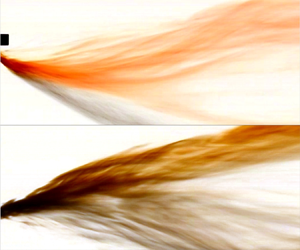
The final case we have considered occurs when the initial net buoyancy of the plume is positive. In this case, the plume again rapidly adjusts to the speed of the ambient, and then as the flow rises, particles begin to separate from the flow (figure 8a). This leads to an initial phase of transport of particles above the initial discharge depth, and an extended zone of particle separation then develops from the rising plume, as may be seen in the time-averaged structure of the plume (figure 8b). The particle separation appears to occur through a series of discrete coherent clouds of particles, as can be seen in the distinct streaks in this figure and in the series of images in figure 8(c). A small amount of plume fluid is drawn down with these particle plumes, but the majority of the original plume fluid continues to rise as a coherent current-blown plume (figure 8a,c). These discrete clouds do now appear to sediment faster than the individual fall speed of the particles (see figure 8d).
(a) Instantaneous and (b) time-averaged images of a typical laboratory experiment in regime C (experiment  $m$, see table 3). (c) Series of four photographs captured at regular time intervals $\Delta t=1.66$ s and at a fixed location in the laboratory frame during the experiment. (d) Time series of the vertical line of pixels fixed in the frame of the laboratory and marked by the dotted line in (c). The black arrow illustrates the Stokes settling speed of the particles, $v$.
$v$.

As the fall speed of the particles increases, the rate of separation of the particles from the rising plume also increases, and in figure 9(b–e) we illustrate the variation of the time-averaged structure of the plume as a function of the particle fall speed for the cases  $v=6.98$, 2.39, 1.03 and 0.63 mm s $^{-1}$ (see table 3). With a larger sedimentation speed the buoyancy increases more rapidly in the rising plume and, hence, the dyed fluid rises more rapidly with distance and the lateral extent of the particle separation zone becomes smaller. Figure 9(g) shows the position of the centreline of the time-averaged fluid plume, with the depth plotted to the power of 3/2 and the horizontal distance scaled as in the solution for the classical plume shape (1.2). A series of experimental results are shown in which the particle load and the buoyancy of the source fluid are both fixed, while the fall speed of the particles is varied. Two model curves are shown (grey dotted lines): one for the shape of the classical plume based on the buoyancy of the fresh water in the plume, and one based on the total buoyancy of the plume. As the fall speed of the particles increases from very small values of order 0.1 mm s $^{-1}$ (black and dark blue lines) to much larger values of order 10 mm s $^{-1}$ (pink and light blue lines), the locus of the rising plume gradually evolves from the trajectory based on the net buoyancy for which there is little particle sedimentation over the scale of the experiment, to the trajectory based on the fluid, which applies when the particles have separated from the plume.
(a) Time-averaged image of a single-phase plume with a buoyancy flux  $B= B_s$ (experiment $j$, see table 3). (b–e) Time-averaged images of four particle-laden buoyant plumes with identical buoyancy flux $B= B_s-\lvert B_p\rvert$, but different particle sizes (experiments $l$–
$l$– $o$). In (b) the plume is laden with relatively large particles which rapidly settle out of the flow. In (c–e) the size of the particles is progressively reduced, leading to slower particle sedimentation. Image ( f) shows the time-averaged trajectory of a single-phase plume with a buoyancy flux $B= B_s-\lvert B_p\rvert$ (experiment $q$). (g) Time-averaged trajectories of the plume fluid in experiments $j$–
$j$– $q$. (h) Growth of the radius $\sigma$ with height $z$ in a saline plume (red line, experiment $q$) and in three particle-laden plumes (experiments $l$–
$l$– $o$), as a function of the horizontal distance from the source, $x$.
$x$.

Conditions of eight regime C experiments, in which a buoyant suspension of heavy particles and buoyant fluid is supplied at the base of the tank (see figure 9). Here  $Q_0$ is the source volume flux, $\rho _f$ is the density of the source fluid, $\rho _{amb}$ is the density of the ambient fluid, $B$ is the buoyancy flux of the particle-laden mixture at the source, $B_s$ and $B_p$ are the components of the buoyancy flux associated with the salt and particle content in the source fluid, respectively, $w$ is the speed at which the nozzle traverses the tank, $v$ is the particle settling speed and $d$ is the mean particle size.

As the plume transitions from the particle-laden fresh water plume to the fresh water plume, there is a region in which the plume becomes vertically stratified in particles (cf. figure 9b,c), with a relatively large particle load on the lower side of the plume, as the particles gradually separate from the flow.
While particles separate from the base of the rising buoyant plume, we find that the entrainment of ambient into the plume is reduced, as some of the fluid at the base of the plume is carried downwards with the particles, rather than being mixed into the flow (see figure 9, especially (c), and the cartoon in figure 10). We have measured the standard deviation as a function of depth,  $\sigma$, and from this estimate that $\beta$ has a value of about $0.32 \pm 0.05$, which is somewhat smaller than for a single-phase plume. However, in the early and late stages of the flow, prior to the transition region where much of the particle separation occurs, we find that $\beta$ has values closer to the expected value $\beta =0.4$.
(a) Cartoon illustrating the entrainment of ambient fluid into a single-phase buoyant line thermal. (b) Dense particles settling from the bottom of a particle-laden thermal affect the entrainment of ambient fluid into the thermal, resulting in reduced  ${{\rm d}}\sigma /{{\rm d}}z$ (see figure 9h).

We have also measured the speed of the descending particle clouds which settle from the base of the ascending plume, and found that the speed of these clouds does now exceed the particle fall speed. For example, figure 8(d) shows that the descending clouds of particles below the main rising plume, which appear as downward streaks in the image, are much steeper than the arrow, which corresponds to the Stokes fall speed of the particles,  $v$. If the concentration of particles in the plume is sufficient, then as the particles separate from the lower surface of the plume, they can form convective plumes which settle out faster than the fall speed of the individual particles (see figure 8, cf. Reference Hoyal, Bursik and AtkinsonHoyal et al., 1999a, Reference Hoyal, Bursik and Atkinson1999b). These convective plumes develop either through a double diffusive instability with small particles for which the fall speed is relatively small, or a Rayleigh–Taylor type instability for larger particles. With low settling speeds, the instability results from diffusion of salt across the density interface between the plume and the ambient fluid, so that the fluid at the base of the plume becomes laden with particles as well as saline, and this falls out through the ambient. With higher settling speeds, the instability arises as particles sediment from the plume and form a particle-rich layer below the plume, which is unstable to a Rayleigh–Taylor instability, as described by Reference Hoyal, Bursik and AtkinsonHoyal et al. (1999a, Reference Hoyal, Bursik and Atkinson1999b) and modelled numerically by Reference Burns and MeiburgBurns and Meiburg (2012, Reference Burns and Meiburg2015). Analogous sedimentation processes happen as sediment separates from fresh river water as it spreads out over relatively brackish sea water (Reference Jazi and WellsJazi & Wells, 2020; Reference Parsons, Bush and SyvitskiParsons et al., 2001; Reference Wells and DorrellWells & Dorrell, 2021). In the present experiments there is some plume fluid carried down with the particle clouds, but the particles do fallout from the lower surface of the plume into the underlying ambient, and so this suggests that the instability is transitional between the double diffusive fingering and the Rayleigh–Taylor regimes (cf. Reference Burns and MeiburgBurns & Meiburg, 2015); we plan to explore this in more detail with further experiments.
4. Modelling the flows
The experimental results shown in § 3 illustrate some of the complexity of the plumes owing to the sedimentation and the associated change in the buoyancy. A comparison of the trajectory of the time average of the fluid plume with the classical single-phase model suggests that the early and late time behaviour, based on the total buoyancy or the buoyancy associated with the source fluid, provides a good representation of the trajectory of the plumes. However, the intermediate flow regime where the sedimentation speed is comparable to the plume speed, is more complex.
In the case of a descending plume, the particles gradually separate from the flow once the descent speed of the flow falls below the sedimentation speed. As an idealised model to illustrate the transition in the flow, we now explore a time-averaged and depth-integrated picture in which we assume the plume moves horizontally with the speed of the ambient fluid, and descends according to the buoyancy force (cf. Reference Hewett, Fay and HoultHewett et al., 1971; Reference Woitischek, Mingotti, Edmonds and WoodsWoitischek et al., 2021), but we also include a simple parameterisation for the loss of particles from the flow based on a horizontally integrated model of the plume. Although the entrainment is suppressed by about 5 %–15 % in the sedimentation zone (cf. figures 4(c) and 9(h)), for simplicity, we assume that the plume radius  $r$ increases linearly with height $z$ (see (3.1)), while the momentum and buoyancy evolution of the flow are given by
 \begin{equation} \frac{{{\rm d}} (r^{2} u)}{{{\rm d}}z} = \gamma (g'_s + g'_p)r^{2}, \end{equation}
where  $\gamma$ is a constant associated with the effective buoyancy force averaged over the plume, which has been shown to have a value of $0.87\pm 0.05$ by Reference James, Mingotti and WoodsJames et al. (2022) for a single-phase plume, and
 \begin{equation} \frac{{{\rm d}} (r^{2} g'_p)}{{{\rm d}}z} = {-}2 r U g'_p, \end{equation}
where for the descending particle plumes, such as those discussed in § 3.1, the net sedimentation velocity  $U$ in (4.2) is defined as $U = v-u$ if $v > u$ or as $U=0$ if $v < u$, where $v$ is the particle fall speed and $u$ is the plume speed (cf. (1.1)); this phenomenological law accounts for the possible reincorporation of particles if the plume descends more rapidly than the particles which sediment from the lower part of the plume. The loss term in (4.2) accounts for the sedimentation of particles from the base of the flow, where $g'_p$ represents the buoyancy of the particles. Without the loss term, these equations have a solution given by (1.2). We have solved the two relations (4.1)–(4.2) alongside (3.1) using the source buoyancy flux and particle load in order to determine the trajectory of the plume, $z(x)$; (3.1) enables us to convert the radius of the plume to the depth of the centreline, by taking the empirical value for $\beta$ as measured in the experiments. In figure 11 we present model predictions for the shape of the plume as a function of the distance along the tank for the case of (i) a dense plume composed of dense fluid and particles (experiment $c$, table 1), and (ii) a buoyant plume composed of buoyant fluid and particles (experiment $n$, table 3). The model captures the main trend of the centreline of the plume trajectory and similar agreement arises for the other experiments. For the experiments with reversing buoyancy (regime B), the model can capture the initial descent of the plume, but does not capture the motion of the fluid as it slowly peels off and rises, since this leads to a distributed zone of fluid rather than a localised buoyant plume (see § 3.2).


5. Effects of stratification
As mentioned in the introduction, the stratification of the water column can also have a significant impact on the plume evolution. The experiments shown in §§ 2–4 do not account for the stratification, but we can draw from these experiments to interpret how the stratification might affect the results. Owing to the stratification, as the plumes migrate vertically, their net buoyancy gradually decreases. Eventually this may arrest the vertical motion of the plume (cf. Reference Mingotti and WoodsMingotti & Woods, 2019, Reference Mingotti and Woods2020; Reference Muñoz-Royo, Peacock, Alford, Smith, Le Boyer, Kulkarni and JuMuñoz-Royo et al., 2021; Reference Wang, Adams, Munoz-Royo, Peacock and AlfordWang et al., 2021), and the subsequent flow will follow the ambient current, with the plume intruding at the level of neutral buoyancy and particles then sedimenting from this flow.
5.1 Two-layer stratification
In order to illustrate some of the effects of stratification, we have run a number of experiments with a two-layer stratification, in which the ambient contains a layer of denser fluid underlying a layer of less dense fluid. This two-layer stratification can arrest the flow if the bulk density of the plume at the level of the interface,  $\rho _P$, lies between the density of the upper and lower layers, $\rho _U$ and $\rho _L$, respectively: in this case, the plume spreads along the interface between the two layers of ambient fluid. However, the net buoyancy of the plume decreases as a result of particle sedimentation, and so we expect the eventual fate of the liquid in the plume to depend on the density of the plume fluid, $\rho _F$, relative to the density of each layer of ambient fluid.
There are a number of possible regimes which the flow can follow, both in the case of a descending and an ascending particle-laden plume. These are illustrated in figure 12(a,b). In figure 12(a) we consider the case of a descending plume and illustrate how the net buoyancy of the plume evolves as a result of mixing in the upper layer, as a function of the salinity of the plume fluid and the particle load. The horizontal axis in figure 12(a) shows the buoyancy associated with the particle load in the plume, while the vertical axis shows the buoyancy associated with the salinity of the plume fluid. Two critical values are identified on the vertical axis, at which the plume fluid depleted of all particles has the same density as the ambient fluid in the upper and lower layer ( $\rho _F=\rho _U$ and $\rho _F=\rho _L$, respectively, horizontal dashed lines in figure 12a). The two dashed inclined lines show the conditions for the bulk density of the particle-laden plume to be equal to the density of the ambient fluid in the upper and lower layer ( $\rho _P=\rho _U$ and $\rho _P=\rho _L$, respectively). Two possible plume mixing lines (thick black arrows) are presented in figure 12(a), assuming there is no sedimentation of particles from the plume. The mixing line A shows a descending plume which initially contains fluid of a larger density than the upper layer ambient fluid. As the plume descends and entrains fluid from the upper layer, the buoyancy of the plume fluid evolves towards that of the upper layer fluid, first crossing the horizontal dashed line at which the salinity of the plume fluid matches that of the lower layer ( $\rho _F=\rho _L$), and then crossing the inclined dashed line at which the bulk density of the plume matches the density of the lower layer ( $\rho _P=\rho _L$). If the plume reaches the interface with the lower layer at a point (i) prior to reaching the horizontal dashed line in figure 12(a), then the flow remains dense and continues through the lower layer. Also, in this first regime the density of the plume fluid at the interface exceeds that of the ambient fluid in the lower layer, and so the plume fluid will eventually continue to descend through the lower layer once particles have sedimented from the flow (cf. figure 3). If the plume reaches the interface at a point (ii) after crossing the horizontal dashed line but before crossing the inclined dashed line in figure 12(a), then the bulk density of the particle-laden plume at the level of the interface exceeds that of the ambient fluid in the lower layer, and so the plume crosses the interface and descends into the lower layer. However, in this second regime the density of the plume fluid at the interface is lower than that of the ambient fluid in the lower layer, and so we expect that, following particle sedimentation, the descent of the residual fluid in the plume will be arrested and the fluid will rise back up towards the interface, in a similar fashion to that depicted in figure 6. Finally, if the plume reaches the interface at a point (iii) after crossing the inclined dashed line in figure 12(a), then the bulk density of the particle-laden plume at the level of the interface is lower than that of the ambient fluid in the lower layer. As a result, the plume intrudes at the interface. As it spreads out along the interface, particles sediment from the flow, but the residual fluid remains denser than the upper layer, and so the plume fluid will remain confined to the interface even after particle fallout. An experiment illustrating this regime is shown in figure 13(a).
Illustration of the different regimes which characterise the flow of (a) a descending or (b) an ascending particle-laden plume in an environment with a two-layer density stratification.

Instantaneous and time-averaged images of two particle-laden plumes descending through an environment with a two-layer density stratification in (a) regime (iii) and (b) regime (iv) (see figure 12).

The mixing line B in figure 12(a) shows a descending plume which initially contains fluid of a lower density than the upper layer fluid, but a sufficiently large concentration of particles, so that the bulk density of the plume exceeds that of the upper layer. Again, as a result of entrainment and mixing, the buoyancy of the plume fluid evolves towards that of the upper layer fluid. It follows that the density of the plume fluid at the level of the interface will be lower than that of the ambient fluid in the lower layer; however, depending on the particle load, the bulk density of the plume may either be larger or smaller than that of the lower layer upon reaching the interface. If the particle load is sufficiently large that the bulk density of the plume exceeds that of the lower layer fluid, then the plume will cross the interface and descend into the lower layer, as discussed above (regime (ii)). However, for sufficiently small particle loads, the bulk density of the plume fluid and particles will be less than the lower layer at the interface, and so its descent will be arrested there. In this fourth regime, denoted by (iv) in figure 12(a), the plume forms an intrusion at the level of the interface. Following particle sedimentation, the residual plume fluid becomes less dense than the upper layer fluid, and so it rises from the interface into the upper layer. An experiment illustrating this regime is shown in figure 13(b).
In the opposite case that there is an ascending plume, there are three different regimes to consider as shown in figure 12(b). The mixing line C corresponds to a plume which is initially buoyant and rises through the lower layer, and so the buoyancy of the plume fluid evolves towards that of the lower layer fluid as a result of entrainment and mixing. If the plume reaches the interface at point (v) in figure 12(b), the plume fluid is denser than the upper layer fluid at the interface. Hence, the bulk density of the plume is also larger than that of the upper layer fluid, and so the particle-laden plume spreads out at the level of the interface. During the subsequent motion, as the particles progressively sediment from the plume, the plume fluid remains trapped at the interface height, analogously to figure 13(a). If the rising plume reaches the interface at point (vi) in figure 12(b), then the bulk density of the plume is still larger than that of the upper layer fluid at the level of the interface, and so the plume forms an intrusion there. However, the density of the plume fluid is now lower than that of the upper layer fluid, and so following particle sedimentation, the residual plume fluid rises above the interface into the upper layer as in figure 13(b). Finally, if the plume reaches the interface at point (vii) in figure 12(b), then the bulk density of the plume at the level of the interface is lower than that of the upper layer fluid, and so the plume as a bulk crosses the interface and rises into the upper layer, with the particles sedimenting from the flow in a fashion similar to that shown in figure 8.
These experiments and regime diagrams illustrate that the presence of stratification can arrest the vertical motion of the plume, and that the plume may then spread out along the level at which the density is intermediate between the adjacent fluid layers. We note that some of the particle sedimentation processes change as a result of the stratification, since the convective plume motion is arrested by the stratification. If particles settle into the underlying fluid this can then generate small dense particle clouds which may fall out at a faster speed than the sedimentation speed, as discussed by e.g. Reference Hoyal, Bursik and AtkinsonHoyal et al. (1999a), Reference Hoyal, Bursik and AtkinsonHoyal et al. (1999b), Reference Parsons, Bush and SyvitskiParsons et al. (2001), Reference Sutherland, Gingras, Knudson, Steverango and SurmaSutherland, Gingras, Knudson, Steverango, and Surma (2018) and Reference Fries, Lemus, Jarvis, Clarke, Phillips, Manzella and BonadonnaFries et al. (2021).
5.2 Continuous stratification
In the case of a continuous stratification, as characterised by the Brunt–Väisälä frequency  $N$, the stratification can again act to stop the motion of the plume and cause a transition in which the flow moves downstream at the neutral buoyancy level. In the case of a descending plume in a relatively strong ambient current, depending on how soon the plume reaches the neutral buoyancy level, the fraction of sediment which has separated from the plume prior to reaching the neutral buoyancy level may vary. For a plume which is swept downstream with negligible particle fallout, the plume radius and vertical speed are given by the model relations (cf. Reference James, Mingotti and WoodsJames et al., 2022)
 $$\begin{gather} \frac{{{\rm d}}b}{{{\rm d}}z} = \beta, \end{gather}$$
 $$\begin{gather}\frac{{{\rm d}}\left(ub^{2}\right)}{{{\rm d}}z} = g'b^{2}, \end{gather}$$
 $$\begin{gather}w \frac{{{\rm d}}\left(g' b^{2}\right)}{{{\rm d}}z} = {-}2 N^{2} b \beta, \end{gather}$$
where the last equation accounts for the changing buoyancy of the plume fluid owing to the entrainment of the stratified ambient fluid. These relations have solution for the buoyancy
 \begin{equation} r^{2} g'(z) = \frac{B_0}{w}- \frac{N^{2}}{3\beta}\left(r^{3}(z)-r^{3}(0)\right), \end{equation}
where  $B_0$ is the buoyancy flux of the source, and this identifies that the depth of the neutral buoyancy level is approximately
 \begin{equation} z \approx \left(\frac{3 B_0}{\beta^{3} w N^{2}}\right)^{1/3}, \end{equation}
while the depth at which the downward speed of the plume matches the fall speed is
 \begin{equation} z\approx 0.5 \left(\frac{B_0}{w v^{2}}\right). \end{equation}
In figure 14(a) we illustrate the depth at which the plume reaches its neutral buoyancy level neglecting the effects of sedimentation (black lines, plotted for two different values of  $N$) and the depth at which the plume speed matches the fall speed of the sediment, at which point sedimentation will start (red lines, plotted for two different values of $v$) as a function of the buoyancy flux $B_0$, for a fixed value of the current speed $w$. It is seen that with larger buoyancy fluxes, corresponding to larger discharge rates, or with smaller fall speeds, corresponding to smaller particles, the effect of ambient stratification may dominate the effect of sedimentation as the plume descends, leading to the arrest of the vertical motion before there has been significant sedimentation. In this case, the sediment will subsequently separate from the laterally spreading intrusion.
(a) We use black lines to show the depth of the neutral buoyancy level (estimated using (5.3)) as a function of the source buoyancy flux  $B_0$ for two different values of $N^{2}$. We compare these depths with the depths at which the downward speed of the plume matches two different particle fall speeds $v$ (red lines, plotted using (5.4)). In plotting all curves, we have assumed $w=0.05$ ms $^{-1}$ and $\beta =0.4$ (cf. Reference James, Mingotti and WoodsJames et al., 2022). (b) Vertical and horizontal extents of a full-scale plume in the ocean as recorded during a field experiment presented in Reference Muñoz-Royo, Peacock, Alford, Smith, Le Boyer, Kulkarni and JuMuñoz-Royo et al. (2021). The black lines illustrate the predictions of the original model developed in Reference Muñoz-Royo, Peacock, Alford, Smith, Le Boyer, Kulkarni and JuMuñoz-Royo et al. (2021). The red lines illustrate the predictions of the model developed in the present paper.

There have been some recent field experiments in which a sediment plume was produced in relatively shallow water by a suspension of particles which were discharged for 45 minutes (Reference Muñoz-Royo, Peacock, Alford, Smith, Le Boyer, Kulkarni and JuMuñoz-Royo et al., 2021; Reference Wang, Adams, Munoz-Royo, Peacock and AlfordWang et al., 2021). In that field experiment, the material was discharged at a depth of 60 m, and the plume was then tracked as it sank through the water. Using the parameter values for that experiment, namely  $B_0 \approx 0.002$ m $^{4}$ s $^{-3}$, $w \approx 0.1$ ms $^{-1}$ and $N \approx 0.01$ s $^{-1}$, and the model presented in this paper, we find that the plume is predicted to descend to a neutral buoyancy depth of about 9–10 m, to have a radius of about 3.5–4 m, as seen in figure 14(b). The shape of the current-advected plume (red lines, illustrating the centre (solid) and edges (dashed) of the model plume) broadly overlaps the acoustic backscatter data reported by Reference Muñoz-Royo, Peacock, Alford, Smith, Le Boyer, Kulkarni and JuMuñoz-Royo et al. (2021), which records the location of the plume in the field experiment.
For this field experiment, the speed of particles is smaller than the fall speed of the plume, and so the particle-fluid mixture is predicted to spread out at the neutral level and then gradually sediment particles (cf. § 5.1). However, if the mass-averaged size of the particles were larger, of the order of a few 100s micron, then the fall speed would be comparable to the plume speed as it approaches the neutral level, and some sedimentation would be expected from the plume. It is relevant to note that on descent, the plume becomes very dilute, but as the plume spreads out at the neutral level, the dynamic mixing will decrease, and most of the subsequent dilution will be associated with ambient turbulence, as the particles gradually settle from the plume.
In plumes with a larger initial vertical speed, comparable or greater than the ambient current speed, the plume will behave in an intermediate fashion between that of a vertical plume or a current-swept plume, as the plume begins to accelerate to the current speed. Depending on the strength of the stratification, this adjustment may not be complete prior to the stratification arresting the flow, and so the dynamics and entrainment process become more complex. A number of authors have explored this transitional regime, using both experiments and parameterised models in which the entrainment is assumed to occur owing to the flow along the axis of the plume as well as across the axis of the plume: this includes the models of Reference Aubry, Jellinek, Carazzo, Gallo, Hatcher and DunningAubry et al. (2017) and Reference Wang, Adams, Munoz-Royo, Peacock and AlfordWang et al. (2021). It would be very interesting to develop the present experimental models of particle-laden plumes for such transitional flow regimes; however, the present results on the mixing and sedimentation which focus on the current-blown end-member provide a valuable reference.
6. Implications of the experiments
During deep-sea mining operations a key priority is to limit the impact of the process on the marine ecosystem and especially that of the sea floor beyond the site of the mine. Our experiments are highly idealised, but illustrate that the initial stages of the transport of particles while being carried by a turbulent, wind-swept plume may be complex, and influenced by the effects of the ambient stratification, sedimentation of particles from the plume and the ambient currents. Combining these effects, we find that the plumes may descend distances of the order 10–100 m, and then intrude in the water column, where the sedimentation, ambient currents and turbulence will then dominate the subsequent dispersal of the particles before reaching the sea floor. In order to model this subsequent transport a regional model of particle transport through the water column is needed, but the present modelling helps to inform the scale and nature of the source conditions for such a model. Once the particles sediment, they will be subjected to the turbulence and mixing in the water column, which may be especially significant in the boundary layer near the sea bed, and this can lead to additional controls on the ultimate pattern of sediment deposition.
The experiments presented in this paper point to some challenges of disposing of particulate waste collected on the mining vessel at the sea surface, since if these particles are to be discharged into the sea, they will typically be discharged in a liquid suspension. The original depth of the sea water used to form this suspension, alongside any temperature changes of this water as it is brought to the surface and mixed with the particles to be discharged from the mining ship, have a critical role in determining the buoyancy of the discharge and, hence, the initial plume dynamics, which also depend on the depth of the discharge point below the surface. In turn, this will influence the fate of any minerals dissolved into the plume water.
In particular, if the water is sourced from high in the water column, this will tend to be buoyant relative to the deeper ocean water. If the particle load is sufficiently high, the discharge plume may initially be dense and so it will fall through the water column towards the neutral buoyancy level. As particles sediment, the residual mixture may then become buoyant and tend to rise up through the water column. In contrast, if the particle load is sufficiently small that the net density of the discharge could be lower than that of the surrounding ambient fluid, and a buoyant plume may form which will rise through the water from the discharge location. To avoid the latter situation, a suspension of dense near-bottom fluid could be mixed with the particles; if the mixture were then to be discharged near the sea floor, this would lead to the mixture sinking to the sea floor as a dense particle-laden plume. If this plume either reached the sea bed or reached its neutral bouyancy level in the deep water a few 10s–100s m above the sea bed, this would then limit the subsequent lateral transport of the particles by the ambient currents and turbulence as they sediment to the sea floor relative to a shallower discharge.
It is of interest to note that the process of sedimentation from the buoyant particle-laden plume (regime C, § 3.3) is also of relevance for volcanic eruption columns in the atmosphere. Such columns consist of hot buoyant air and heavy particles. As the particles settle from the buoyant flow, the remaining fluid rises as in the present experiments. The process of sedimentation of particles from historic wind-swept volcanic plumes suggest that a series of discrete clouds of particles separate from the plume as the remaining flow is carried downwind, as in the photograph from the 1984 eruption of Mount Pagan (figure 15). This is analogous to the process of sedimentation seen in the experimental flows reported herein, e.g. figure 15(b) and has been discussed by Reference Carazzo and JellinekCarazzo and Jellinek (2012), Reference Carazzo and JellinekCarazzo and Jellinek (2013), Reference Manzella, Bonadonna, Phillips and MonnardManzella, Bonadonna, Phillips, and Monnard (2015) and Reference Fries, Lemus, Jarvis, Clarke, Phillips, Manzella and BonadonnaFries et al. (2021). The details of the volcanic plume are more complex owing to the heat transfer from the particles to the air and the associated generation of buoyancy, as well as there being a range of particle sizes: we plan to explore these effects in more detail in future research.
(a) Photograph of an ash plume produced by the May 1994 eruption of Mount Pagan, compared with (b) a photograph captured during experiment  $m$ (see table 3).

7. Summary
Experiments to model the motion of particle-laden, positively and negatively buoyant plumes moving through the ocean in a cross-flow have identified a range of behaviours of the particle-fluid mixture, ranging from (a) buoyant rising plumes, when the fluid in the discharge is buoyant relative to the density of the ambient at the discharge depth and the particle concentration is sufficiently small, to (b) sinking negatively buoyant plumes, when the fluid in the discharge is dense relative to the ambient. The separation of the fluid and particles can lead to a complex spatial distribution of the particles, and potentially large dispersal distances associated with the transport by lateral currents, especially if the plume is buoyant.
We have shown how classical models of single-phase plumes in a cross-flow can describe the motion of the centreline of the plume in the case that the plume descent speed exceeds the fall speed of the particles, and that subsequently sedimentation leads to a change in the buoyancy of the plume, and an associated change in the rate of ascent or descent of the plume fluid. In the case that the plume consists of an initially dense mixture of buoyant fluid and particles, the motion of the fluid is initially downwards, but the fluid then peels off the top of the flow, producing a dispersed zone of rising buoyant fluid, while the particles continue to descend. We have also explored the effects of stratification in the water column and shown that it can also arrest the plume, in which case the sedimentation occurs as the plume intrudes at its neutral buoyancy level, rather than in the descending flow.
Funding Statement
This research was funded by the BP Institute for Multiphase Flow, University of Cambridge, UK.
Declaration of Interests
The authors declare no conflict of interest.
Data Availability Statement
Raw data are available from the corresponding author.
Ethical Standards
The research meets all ethical guidelines, including adherence to the legal requirements of the study country.


 Open access