Introduction

It may be said that of all the forms of frozen water that exist on Earth, the one that we know the least about from a geophysical point of view is (loafing ice. A good example of our paucity of knowledge in this regard is that for the complete I.G.Y. period (1957-58) we know essentially nothing about the extent and morphology of the sea ice surrounding Antarctica. Our ignorance embraces not only such striking macroscale phenomena as the sea-ice canopies that cover vast areas of the world ocean, approximately 10% in the northern and 13% in the southern hemisphere, but also what could be called mesoscale ice areas, such as the sea ice of the Gulf of St. Lawrence and the Baltic Sea and the lake ice of the Great Lakes. Floating ice of all scales undergoes rapid morphological and dynamic changes and is one of the most variable physical features of the Earth’s surface. Our lack of knowledge of this type of ice is not only due to its extent and variability but also because observations have been limited by the environment in which it usually exists—dark and cloudy.

The interest in floating ice by the community of geophysically oriented scientists has blossomed in the last few years. Investigations of climate variations have laid new stress on the need to treat the atmosphere-ocean-ice-land system as a whole and to acquire sequential synoptic data on the large floating and grounded ice masses that are involved in a complex feedback process with atmospheric and oceanic circulation. This interest has led to the creation of the two international research programs concerned with floating ice: the Arctic Ice Dynamics Joint Experiment (AIDJEX), which seeks to develop numerical models for the dynamics and thermodynamics of sea ice, and the Polar Experiment (POLEX), which seeks to improve our understanding of how polar sea- and glacier-ice canopies are related to climate variations on the time scale of seasons to decades. Both of these programs place strong emphasis on the need to study floating ice with remote-sensing techniques. Indeed, satellite remote sensing offers the only feasible means of acquiring the macroscale sequential synoptic data needed to test existing and developing climate models.

The recent efforts by many nations rapidly to exploit oil resources in the Arctic and sub-Arctic and to extend the navigable season in ice-infested waters has placed further emphasis on the need for ice observations by remote sensing. Iceberg tracking by satellite has been done by using both sequential imagery and positioning platforms—measurements which are needed for the possible towing of icebergs as a water resource and for preventing them from colliding with man-made structures.

This recent increased interest in floating ice has occurred during a time of rapid evolution of both remote-sensing sensors and platforms. Because of this the general ice investigator finds himself faced with a panoply of possible data to aid him in his research, but he has not had sufficient information about many of these data to allow him to make a discerning choice concerning its applicability to the particular problem that he wishes to resolve. Therefore, we wish in this paper to discuss recent developments in remote sensing of floating ice by means of visible, passive microwave, and active microwave techniques, the way they have been used in recent experiments such as BESEX (Bering Sea Experiment), the AIDJEX pilot studies, and Skylab, and what new possibilities are in the offing.

Visible sensing

Within the last two years there have been large advances in utilizing satellite “visual” imagery to investigate different aspects of the geophysical behavior of sea ice. Even before this period, satellite observations of sea ice had proven to be very useful (Reference Wark, Popham, Wexler and Caskey, J. E.Wark and Popham, 1963; Reference McClain and BockMcClain and Baliles, 1971; Reference Aber and VowinckelAber and Vowinckel, 1972; Reference Barnes, Barnes, Chang and WillandBarnes and others, 1972). However, the data collected by the earlier meteorological satellites had serious limitations as far as quantitative geophysical investigations of sea ice were concerned. This was primarily caused by the resolution of the resulting imagery, which was such that only gross ice features such as the overall boundaries between pack ice-open water could be distinguished. Small-scale features which would have provided information on the geometry of the leads and floes were simply not observable. Also, in many cases the imagery was difficult to register exactly on an easily usable map projection. However, when ERTS-I was launched in July 1972 all this changed.

ERTS (Earth Resources Technology Satellite)

ERTS imagery is of cartographic quality with very little distortion on a scale of 1: 10⁶, In addition, the images produced by the multi-spectral scanning system (MSS) on the satellite reveal a wealth of information on each image containing sea ice. Because of this, the first studies utilizing ERTS to investigate sea ice were focused on establishing exactly what useful ice features could be observed (Reference Barnes, Bowley and FredenBarnes and Bowley, 1973, Reference Barnes, Barnes, Bowley, Chang, Willand, Santeford and Smith1974; Barnes and others, 1974; Campbell, 1973). The list has proven to be quite impressive. Sea ice can readily be identified in all the MSS spectral bands because of its high reflectance. However, bands in the visible range (MSS 4 and 5, 0.5-0.6 and 0.6-0.7 μm) are the most useful for mapping ice edges and detecting thin ice. MSS 7, on the other hand, which is in the near-IR range (0.8-1.1 μm), is most useful for identifying features which are revealed by changes in the ice surface characteristics. Because high-contrast linear features at least as narrow as 70 cm can be observed, ERTS imagery is ideal for studies of lead patterns and floe size distributions. Also, the different classes of thin ice (open water, grey ice, grey-white ice) can be noted and distinguished from thicker ice. However, at the present the correlations between reflectance levels and actual thin ice thicknesses are qualitative. In addition, melt water on the ice surface is indicated by its very low reflectance in the near-IR, brash ice can be distinguished from other ice types, and in a few cases old ice can be separated from first-year ice. In short, although there are a number of important common ice features that cannot be distinguished on ERTS imagery (ridges, hummocks, rafted ice, individual melt features, and in most cases old ice), ERTS imagery clearly contains a wealth of information on ice types, concentrations and deformation patterns that can be treated in a quantitative way.

There are, however, three problems with ERTS as applied to sea ice: it is limited by cloud cover, by lack of daylight, and by the timing of the imagery taken of a given spot on the Earth’s surface. At the equator, ERTS returns to cover exactly the same area once every 18 d. Because of the dynamic nature of sea-ice drift, such a data spacing would clearly be inadequate to investigate more than the gross seasonal changes in ice distribution. Fortunately, however, because ERTS is in a near-polar orbit, in the high latitudes the orbital overlap results in sequential images during three to four consecutive days during the 18 day repeat period. It is this sequential imagery that is most useful for detailed studies of ice motion.

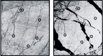
Fig. 1. Enlarged portions of ERTS-1 images 1239-21461-7 and 1242-22032-7, showing the old fracture patterns that were utilized in specifying strain-array points (Reference Crowder, Crowder, McKim, Ackley, Hibler, Anderson and SantefordCrowder and others, 1974). The first image (a) was obtained on 19 March 1973 end the second (b) on 22 March 1973. The width of each image is 34 km.

There are, however, two changes that could be made in the ERTS operations routine that would improve sea-ice data acquisition. The satellite could be left on at lower light levels than those under which it usually is operated when over more equatorial areas. The surface of sea ice is one with a very high reflectance. Leads and thin ice, on the other hand, have a low reflectance. Because of this high contrast, preliminary observations suggest that it is possible to obtain useful data on sea ice under light conditions that would be inadequate for normal scanner operations over more typical terrain. This would allow an expanded period of data acquisition both going into and coming out of the winter dark period. Also, ERTS imagery is, at present, only obtained on ascending satellite passes, while the descending passes are used for data transmittal and orbit adjustments. It should, in principle, be possible to obtain imagery on both descending as well as ascending passes over the polar regions. This would double the amount of potential imagery that could be obtained during a given period, thereby increasing the chances of obtaining both cloud-free conditions as well as a sufficiently detailed image set to specify interesting ice changes clearly. Sea ice is rather unusual in this respect in that it is one of the few Earth surface features that change with sufficient rapidity to make a sampling interval of 12 to 48 h near to ideal.

Although the utilization of ERTS imagery to study the geophysical aspects of sea ice is just starting, nevertheless, there have already been several interesting studies directed toward measuring sea-ice drift and deformation in the coastal regions of the Arctic quantitatively. Such utilization is particularly simple in that coastal features can be used to position the imagery so that absolute movements of identifiable ice features can readily be measured. Unless there is an extensive cloud cover, it has, fortunately, proven to be easy to obtain large numbers of identifiable features that can be used as strain-array points. This is clearly shown in Figure 1 (Crowder and others, 1974), which shows two images separated in time by three days taken just north-cast of Barrow, Alaska. The uncertainty in fixing the position of each point is believed to be roughly too m on a working scale of 1 : 10⁶. In most studies, the transfer points have been located on old lead systems within floes or on irregularities on the edges of current floes. Figure 2 shows the deformation of ice in the shear zone north-cast of Barrow on 22 March 1973 (Crowder and others, 1974; Hibler and others, in press). The indicated array of points was established three days earlier on 19 March as two nested circles with diameters of 33 and 79 km respectively. Using the successive portions of each of the 21 identified ice positions, least-squares estimates of strain-rates and vorticity could be obtained. Information could also be gathered on the inhomogeneous nature of the ice velocity field. The observations suggest that the pack is essentially trying to rotate clockwise as a whole. This in turn requires that the bond to the shore ice be broken. Typical strain-rates were as much as five times higher than strain-rates measured away from the shore in the main ice pack. It was also possible to study the behavior of ice as a function of distance from the edge of the fast ice. As one moves north, the shear first has a large negative value (i.e. the ice near shore moves slower than the ice further north) before becoming positive at distances of about 60 km off-shore. This was true in all of the imagery examined. Again this suggests that the pack as a whole is rotating clockwise with the slip concentrated in a narrow band near the fast-ice boundary. The near-shore shear values are also much larger than values obtained within the main ice pack by using direct deformation measurements on the ice (Reference Hibler, Hibler, Weeks, Ackley, Kovacs and CampbellHibler and others, 1973, Reference Hibler, Hibler, Weeks, Kovacs and Ackley1974).

These studies provide valuable information on how best to formulate reasonable boundary conditions for the behavior of the Arctic pack in the highly deformed near shore region. The current results suggest that the assumption of no slip at the boundary, coupled with a single value for the ice viscosity, definitely does not appear to be realistic. Hibler and others (in press) have suggested that either a two-viscosity model or a model allowing for boundary slip are possible alternatives, while Rothrock (in press) has argued that the assumption of a plastic ice behavior best accounts for the behavior as observed via ERTS.

A somewhat similar study has been carried out in the vicinity of the Bering Strait by Shapiro and Burns (in press) for the time period 6-8 March 1973. In this study, the ERTS imagery was also supplemented by imagery obtained by the Defense Meteorological Satellite Program (DMSP) to provide both qualitative information on the general ice movement and the location of the edge of the ice pack in the southern Bering Sea at the time of the detailed observations in the vicinity of the Bering Strait. During the complete 10 d period covered by the DMSP imagery, a southerly ice movement through the Straits was observed. The 2 d period covered by ERTS revealed individual flow drifts of as much as 50 km. Figure 3 shows the ice displacement vectors determined for the time period between 6 and 7 March 1973. The maximum ice movement during this time was 35 km. Associated with this drift pattern, a zone of intense lead development was observed extending as far as 250 km north of the Bering Strait. The lead pattern could best be described as a series of east-west trending tension leads bounded by highly deformed shear zones which intersect at the north end of the area of leads. During the brief period of observation, a rapid northward expansion of the zone of leads could clearly be noted. An anology is developed by the authors between the observed lead patterns and the plane-strain slip-line fields that are formed in a perfectly plastic material when it is extruded through a rough, unsymmetric die. This correspondence again supports recent work suggesting that sea ice may very usefully be modeled as a plastic material (Coon and others, 1974).

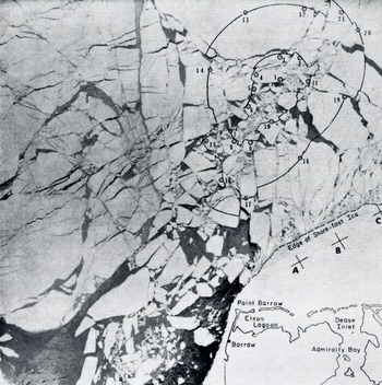
Fig. 2. ERTS-1 multispectral image 1242-22032-7 (Band 7) taken 22 March 1973, showing the deformation of the off-shore pack near Barrow, Alaska (Crowder and others, 1974; Hibler and others, in press).

Another interesting study using ERTS is by Ramseier and others (in press) who have utilized the "quick-look" imagery to investigate the possibility of obtaining nearly real-time information on ice dynamics within the channels of the Canadian Archipelago and the near-shore portions of the Arctic Ocean. Even from this preliminary study, valuable information on ice drift within the Arctic Islands could be determined. For instance, it has been possible to obtain velocity vectors Tor ice movement over wide areas within the islands. These observations show that there are very broad patterns of ice drift even within these channels, with the general ice motion being to the south. This drift transports heavy multi-year ice from the Arctic Ocean towards Viscount Melville Sound. The details of the velocity field may, however, be quite complex. For instance, Figure 4 shows ice movements to the west of Ranks Island that are completely counter to the generally clockwise rotation of the Pacific Gyre.

Fig. 3. Ice drift displacement vectors as determined from sequential ERTS imagery for the time interval 6-7 March in the vicinity of the Bering Strait. Each vector represents a change in position of either an individual floe or a recognizable point on a larger ice mass. The scale of the vectors is the same as the map scale. The general ice motion is always toward the south. The dotted line indicates the edge of the fast ice (Shapiro and Burns, in press).

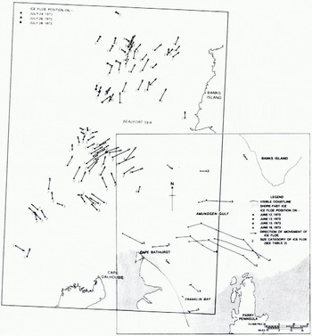
Fig. 4. Ice drift vector mop of the eastern Beaufort Sea, 24-28 July 1973, and Amundsen Gulf, 12-16 July 1973 (Ramseier and others, in press).

All the above studies are extremely encouraging in that they clearly show that valuable quantitative information on the geophysical behavior of the sea ice in the near-shore regions can easily be obtained from ERTS. Because of the highly deformed nature of this ice, more conventional ice-based operations such as those employed by AIDJEX would be both dangerous and expensive.

As noted, all the above studies use shore-line features to align the images. When ice conditions away from the coast are the subject of study, this type of alignment is not possible and it is necessary to position the image on the Earth’s surface by using information calculated from the satellite orbit. Expected errors in this procedure are roughly 2 km, with occasional errors as high as 8 km being noticed (Reference NyeNye, 1975). Relative strains, on the other hand, can be measured with an error similar to that obtained by near-shore studies. As Nye points out, because a reference feature on the ice invariably changes with time; if the length of the observation period is lengthened, one first gains in precision because of the usual increase in strain with time, then one loses precision because of the loss of detail in the reference points. The results of preliminary work near the area of the 1972 AIDJEX camp have been quite encouraging in that it has been possible to spot identical features on images taken as much as 17 d apart (7 and 24 May 1973). Study of a variety of images taken during this period have shown that there was a variation of ice velocity on a spatial scale of roughly 500 km with smaller-scale variations superimposed upon this. The large-scale variations ranged from 0 to 8 km d^-1, while the small-scale variations averaged about 0.3 km d^-1. These small-scale variations are not believed to be produced by measurement errors, but are considered to be the result of the inhomogeneous nature of the deformation field in the sense discussed by Hibler and others (1974). The strain-rates calculated from the large-scale velocity variations ranged between 0 and 2.5% d^-1. Nye was also able to examine the effect of the length of the strain line on the observed strain-rates. As might be anticipated by the direct laser strain studies of Hibler and others (1974), the scatter of the individual estimates around the smoothed strain values decreased as the gauge length increased, with the scatter becoming roughly constant at gauge lengths of at least 50 to 100 km. These results suggest that while a gauge length of 50 km may give a strain-rate that differs from the regional average by as much as 1% d^-1, the corresponding variation for a gauge length of 100 km is only 0.4% d^-1.

It is, of course, these large-scale variations that are relevant to numerical ice deformation models such as the one being developed by AIDJEX. These results are most encouraging in that they suggest that a continuum model for ice deformation does appear to be justified on a gauge length scale of 100 km, in that small-scale variations related to floe-floe interactions do not obscure the large-scale trends at this scale.

In conclusion, the scale and the detail of ERTS imagery are ideal for studying sea-ice dynamics on a geophysical scale that has never before been accessible. The fact that there are 14 d holidays in the data, and that ERTS does not penetrate clouds, are, of course, significant drawbacks. However, the preliminary studies described here are so encouraging that further quantitative studies of sea ice based on ERTS must clearly be ranked as of paramount importance for investigators interested in sea ice. ERTS will clearly provide much of the “ground truth” against which dynamics models of sea ice will be tested.

NOAA-2

Following ERTS, the next most important satellite obtaining imagery in the visual range is NOAA-2. This satellite, which is also in a near-polar orbit, carries a scanning radiometer (SR) as well as a very high-resolution radiometer (VHRR) and obtains a complete coverage of the polar regions every one to two days. The following brief description of the sensing systems aboard the satellite is taken from McClain (1974, [a], [b]).

The two-channel SR was originally designed for twice-daily global-scale cloud mapping as well as for simple direct local readout by ground stations. Its visible-band detector is sensitive to reflective solar radiation for wavelengths from 0.5-0.7 μm. Its nominal ground resolution is 3.5 km at nadir. The thermal IR detector measures the back radiation from the clouds and from the Earth’s surface in the range between 10.5 and 12.5 μm in order to minimize atmospheric attenuation. The resolution of the IR channel of the SR is 8 km. Because of its resolution, the SR is primarily useful in mapping the changes in gross features such as the boundary of the pack ice or the shape and size of large polynyas.

The VHRR images which cover a 2 000 km X 2 000 km area per picture are more limited than is the SR (i.e. imagery is available every two days as opposed to twice daily). However the VHRR resolution is significantly higher (1 km on both the visual and IR) resulting in a four-fold improvement over pre-ERTS visual imagery and a 10-fold improvement over prior IR measurements. Although the VHRR was designed as a direct read-out system there is also a limited data-storage capability of roughly 8% of the daily data load. This capability has been used to obtain glaciological observations in the Ross and Weddell Seas as related to both ship routing and the tracking of large ice floes and tabular icebergs (Reference DeRyckeDeRycke, 1973). In the northern hemisphere, reasonably complete VHRR coverage is available over the whole of the North American Arctic from Greenland in the east to the Bering Sea in the west. It should also be noted that since late 1973 the quality of the VHRR images being produced has been enhanced by distributing the 16 distinguishable grey tones over the temperature range normally experienced in the polar regions (≈ 30 deg) as opposed to the usual range of 100 deg that is utilized for meteorological purposes.

The advantages of NOAA-2 imagery as compared to ERTS are that it is capable of providing regular 1 to 2 d broad-scale coverage of the polar regions during both the light and dark periods of the year. The disadvantages of the imagery are that associated with the increase in scale there is a loss of detail with only the larger of the open-water and thin-ice areas showing. Nevertheless there are usually enough large leads so that the general deformation patterns appear to be revealed reasonably well. However, the current projections of the NOAA-2 VHRR images are such that transfers to a more standard map projection are difficult without an appreciable loss of information. Also NOAA-2 imagery is, as is the ERTS imagery, limited by cloud cover. As analysis of satellite imagery continues, probably one of the most useful purposes of the NOAA-2 imagery will be to provide the broad semi-quantitative “picture” of the behavior of the overall ice pack within which the details as documented by either ERTS or high-elevation aircraft missions can be interpreted in a meaningful way.

At the present time, there have been three principal attempts to utilize either NOAA-2 or similar quality imagery to study the geophysical behavior of sea ice. In the first of these, Reference WendlerWendler (1973) has examined the variations of the ice conditions within a small 120 km × 150 km area located just off-shore north of Barter Island, Alaska. The actual imagery used was obtained by the advanced Vidicon camera system (AVCS) aboard ESSA-9. This AVCS imagery has a similar resolution to the SR imagery produced by NOAA-2. First 5 d minimum brightness composites were prepared for the lime period between 17 May and 17 September 1969. Based on these composites, five categories of ice cover were distinguished ranging from open water to very compact ice with a dry snow cover. Maps were then prepared of the distributions of these ice categories during the period of the summer and changes in these distributions were examined in the light of changes in the wind field as determined from surface pressure charts. As might be expected, off-shore winds moved the ice away from the shore while on-shore winds brought it back. Comparisons were also made with ice conditions as reported on ice charts of the more conventional type based on aircraft observations, and, in most cases, good agreement was found. Wendler was also able to prepare monthly mean albedo maps of the area under study by assuming that there is a linear relationship between reflected energy and brightness in the range 10 to 85%.

The second study (Ackley and Hibler, in press) examines 15 NOAA-2 images obtained over the Beaufort Sea during March 1973 and explores the relationship between the observed ice deformation and the changes in the atmospheric pressure field. First it is hypothesized that changes in the area of “open” water as seen in the imagery can serve as a direct measure of the divergence of the ice. The problems here, of course, are that the sizes of a number of leads of interest are below that resolvable on the imagery and that thin new ice can be mistaken for open water. Therefore, it was decided to use a parameter that could readily be measured from the imagery (i.e. the lead density) and utilize it as an index of divergence. This is qualitatively reasonable inasmuch as narrow fractures will widen and appear on the imagery as divergence progresses while with convergence fractures will disappear. During the period of study, a large, complex lead system developed in the study area indicating intense ice deformation. One triangular lead was noted that was over 200 km long and over 75 km across at its widest point. Estimated divergence rates over one 4 d period were as large as 0.009 ^h-1 which is an order of magnitude larger than values obtained from recent field measurements (Hibler and others, 1974). Attempts were also made to correlate the negative Laplacian of the atmospheric pressure field, which provides a measure of the divergence of the wind velocity field, with the estimated ice divergence rate. Although large values of -∇² P corresponded well with large values of the lead density, the overall correlation of the two parameters during the month of observation was poor.

The meteorology during the study period was dominated by an intense (>1 040 mbar) and stable anticyclone centered over the Beaufort Sea. The divergence of the wind field associated with this anticyclone caused the ice to “open up”. Associated with this opening, the “effective viscosity” of the ice is believed to drop causing the opening to accelerate further. Ackley and Hibler suggest that a consequence of a number of such anticyclones occurring during a given winter would be a large increase in ice production and ultimately, an increase in pressure ridging.

Finally, Streten (1974) has examined the temporal and spatial variations in the large polynya (so-called Westwater) that commonly exists south and west of Banks Island. The time period of the study was the spring and summer of 1973, and both NOAA-2 and DMSP imagery were used. It proved possible to map the locations of the notable fracture patterns, the position of the edge of the pack, and the change of the areal extent of the polynya with time. An attempt was made to analyze these observed changes in terms of the wind stress as estimated from 5 d means of lateral differences in the observed atmospheric pressure field. Some general correspondence between the observed ice behavior and the estimated wind stress was found although, as was true in the Ackley and Hibler paper, the correspondence was clearly less than that desired. It should be noted that at least some of this poor correspondence is undoubtedly the result of inadequate meteorological information to specify the pressure field properly.

It is believed that the above papers offer a preview of some of the studies that will occur in the near future relative to sea-ice dynamics. NOAA-2 imagery clearly has its unique set of advantages in its large-scale view, its sufficient resolution to see a number of important deformation parameters, and its year-round coverage.

DMSP and Skylab

Brief mention should also be made here of the potential sea-ice applications of the Defense Meteorological Satellite Program (DMSP) and of Skylab. The DMSP, which has formerly been called Data Acquisition and Processing Program (DAPP), is a meteorological program of the U.S. Department of Defense designed specifically to collect world-wide cloud information. Although some aspects of the DMSP data reduction system remain classified, the resulting imagery is now available to interested users through the Space Science and Engineering Center at the University of Wisconsin (Meyer, 1973; Reference Blankenship and SavageBlankenship and Savage, 1974). There are usually two DMSP satellites operating at any given time with one in a noon midnight orbit and the other in a morning-evening orbit. The imagery is collected by a four-channel line-scan radiometer in both the visual (0.4 to 1.1 μm) and the IR (8 to 13 μm) with each spectral type being separated into resolutions of either 3.7 or 0.5 km at nadir. The normal scale of the imagery is 145 km/cm but an expanded scale of roughly 72 km/cm can also be used. To the best of our knowledge, there have been no detailed studies of sea ice using DMSP imagery. However, in three different cases (unpublished work by W. J. Campbell; Shapiro and Burns, in press; Streten, 1974), this imagery has been used to define the edge of the pack ice while more detailed observations were made within the pack using ERTS or NOAA-2. Figure 5 shows a DMSP image of the Bering and Chukchi Sea areas taken during the joint U.S.-U.S.S.R. Bering Sea Experiment (BESEX). Considering the quality of the imagery as well as its high resolution, the DMSP imagery should certainly be most useful in future sea-ice research.

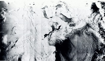
Fig. 5. Visual imagery obtained by lite Defense Meteorological Satellite Program over Bering Sea—Bering Strait-Chukchi Sea region during the BESEX remote-sensing experiment, 18 February 1973. Note that the wind direction is from the north-east as revealed by the roll vortex clouds. This has produced large “open water—thin ice” areas to the lee of the Chukotsky and Seward Peninsulas and Saint Lawrence Island.

Finally, the lake-ice and sea-ice program conducted from Skylab 4 should be mentioned. In contrast to the other satellites discussed here, this satellite was manned by a crew of three astronauts who had been carefully briefed on what sea-ice and lake-ice features they might expect to see. Because the satellites orbit was non-polar, the northern-most position of the satellite was lat. 50° N. Although this ruled out observations on polar areas, it was possible to examine the ice in the Gulf of St. Lawrence, Lake Ontario, James Bay and the Sea of Okhotsk as well as the northern extent of large icebergs in the Southern Ocean. As of the present time, only the "hand-held" camera imagery has been studied (Campbell and others, 1974[b], in press [b]). These photographs have, however, proven to be quite interesting inasmuch as the astronauts attempted to document all the various ice conditions that they encountered. For instance, Figure 6 shows the northwestern port ion of the Gulf of St. Lawrence. Note the presence of a shore lead along the entire north shore of the Gulf. It was found that this lead extended cast to a heavy ice zone which occurs at the neck of the Strait of Belle Isle. Because of the general southerly ice drift during the period of study, the northern edge of the Gulf served as a source area for ice which was then advected to the south. The lead patterns in the figure are quite interesting in that they show a generally extending flow of ice into the Southern Gulf, except in the Jacques Cartier Passage where this flow is blocked by Anticosti Island. This blockage results in north south leads produced by the local compressional flow resulting in lateral divergence to the east and the west. Note also the chevron pattern in the lead structure to the north-east of Anticosti Island and the vortex structure developed in the ice in the lee (to the south) of the island. During the three weeks of the Skylab Gulf experiment, this vortex was continuously developed and the area was one of constant ice production. These photographs should prove to be an invaluable aid in interpreting the results from the Earth Resources Experiments Package (EREP) operated from the satellite, the aircraft remote-sensing data acquired by the four aircraft that participated in the experiment, the ground measurement data acquired from a ship in the Gulf, and the data obtained from a helicopter and hovercraft in Lake Ontario. The imagery also gives an impression of what can be expected from the Apollo Soyuz Program during which a more interesting orbit will be taken that will allow imagery to be collected over the southern readies of the Arctic Ocean. The principal drawback to the Skylab imagery is that every photograph is taken at a different and unspecified angle relative to nadir. This makes the correction of the images to a standard map projection rather difficult. Also, by its very nature, the coverage provided by a camera that must be maimed is inevitably sporadic.

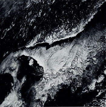
Fig. 6. Hand-held Hasselblad photograph of the Gulf of St. Lawrence taken from Skylab-4 on 20 January 1974. Note the shift in the fracture patterns around Anticosti Island mid the continuous shore lead along the south coast of Quebec (Campbell and others, in press [b]).

Passive microwave sensing

When we consider the whole spectrum of remote-sensing techniques that have been applied to the study of floating ice during the last several years, perhaps the most rapidly evolving and break-through producing area of research has been in the passive microwave region. This is ironic when we recall that the sensors which have proved most useful were designed, built, and flown for studies of atmospheric water. Both aircraft- and satellite-borne microwave radiometers have been used to observe a wide variety of types of floating ice, and although we can speak of this field of research as just getting started, sufficient data exist to make us realize that these measurements will be a fundamental part of future ice research programs. In the following, we present a review of passive microwave studies of floating ice and give examples of the kind of data which will become increasingly more available for ice research in the future.

Arctic Ocean

The most important series of remote-sensing flights which demonstrated the feasibility and usefulness of ice observations by passive microwave sensors were those that took place as part of the AIDJEX-NASA co-operative program. A series of three A1DJEX pilot field experiments were performed during the springs of 1970, 1971 and 1972 in the southern Beaufort Sea, in an area at approximately lat. 74 ° N. running from long. 130 ° W. to 160 ° W. During each of these experiments, the NASA CV 990 “Galileo” aircraft performed a variety of remote-sensing flights at altitudes ranging from 150 m to 10 km. This aircraft was equipped with a wide variety of visual and infrared sensors as well as a 19.3 GHz microwave imaging radiometer and 1.42 GHz, 4.99 GHz, 10.7 GHz, and 37.0 GHz microwave radiometers.

The 1970 “Galileo” flights were made in June north of Point Barrow. The microwave data (Reference Wilheit, Wilheit, Blinn, Campbell, Edgerton and NordbergWilheit and others, 1971, Reference Wilheit, Wilheit, Nordberg, Blinn, Campbell and Edgerton1972) showed that it was possible to distinguish sea ice from liquid water both through the clouds and in the dark. This finding was of great, interest because it pointed the way to an "all-time" ability to observe leads and polynyas in the ice pack. The 1970 data also showed that strong microwave emissivity differences occur on the ice surface itself, but lack of sufficient ground-truth observations prevented a determination of the reason for these differences.

During the 1971 AIDJEX-NASA experiments, a ground-truth program was carried out in conjunction with five “Galileo” overflights. The installation of an inertial guidance navigational system in the aircraft made it possible to fly high-level mosaicing missions in which essentially synoptic microwave maps were made of a large area of sea ice (10 000 km²). Gloersen and others (1973[b]) found that the microwave emissivity differences of the sea-ice surface are associated with the age of the ice, with multi-year sea ice having cold brightness temperatures (≈210 K) and first-year ice having warm brightness temperatures (≈235 K.). This was an important break-through, because it pointed the way to an all-time, all-weather means of distinguishing between old and new ice and tracking ice motion as well as lead and polynya motion.

During the 1972 AIDJEX-NASA experiment a detailed ground-truth program was performed in conjunction with seven “Galileo” flights. A 13.4 GHz microwave radiometer mounted on a sled was used to map the surface brightness temperatures of various ice types and detailed crystallographic measurements were made in each test area. Analysis of these data (Meeks and others, in press) show that surface salinity and pore size are primarily responsible for determining the microwave emissivities of sea ice of various ages. They also show that for mixtures of ice of different ages in which the pieces are small compared to the area sampled by the radiometer beam (footprint), the percentage of multi-year versus first-year ice can be estimated using microwave techniques.

The microwave mosaic maps of the AIDJEX area and of the near-shore marginal ice zone showed that both morphological and dynamical ice features can be observed at all times in any weather. It has even proven possible to make a time sequence of the microwave mosaic maps showing the sea ice extending from Harrison Bay north into the Beaufort Sea for approximately 350 km (see Fig. 7, pl. I). The seven images cover the time from 4 to 23 April 1972. Three distinct zones of sea ice can be observed in each image: (1) a shore-fast zone made up of undisturbed first-year ice having a uniform high brightness temperature; (2) a shear zone composed of three distinct ice types—multi-year floes with cold brightness temperatures, refrozen polynyas with brightness temperatures similar to that of the shore-fast ice, and a mixture of first-year and unresolvable chunks of multi-year ice having a brightness temperature between that of the above ice types; (3) a zone of a mixture of first-year and unresolvable chunks of multi-year ice with many refrozen polynyas. The extremely dynamic nature of the shear zone is clearly seen, with its width doubling in 19 d. Figure 8 shows a series of trajectories of floes deduced from the maps shown in Figure 7. The average drift speed in the shear zone was about 3 km/d to the west while the average drift of the AIDJEX array 150 km to the north was 6 km/d to the west.

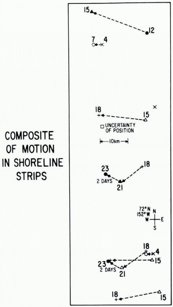
Fig. 8. Ice motion as deduced from studies of the sequential microwave mosaics as shown in Figure 7 (Campbell and others, in press [a].

The first passive microwave imager in space was the electronically scanned microwave radiometer (ESMR) mounted on the NIMBUS-5 satellite which was launched on 11 December 1972. The microwave brightness temperature maps of the Arctic observed by ESMR provide the first synoptic maps of large-scale sea-ice distribution. By using a combination of the AIDJEX-NASA data, ESMR images, and ERTS-1 images, Campbell and others (1974[a]) have shown that the ice cover of the Beaufort Sea is highly heterogeneous, its eastern sector being made up of large multi-year floes and its western sector being made up of a mixture of small, fragmented first-year and multi-year floes.

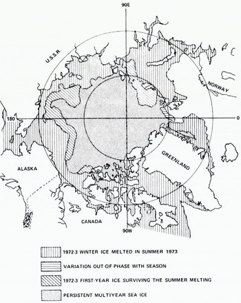
Fig. 10. Near minimum and near maximum Arctic sea ice boundaries for 1973 based on ESMR imagery (Gloersen and others, 1974[a]).

A pair of ESMR images of the Arctic is shown in Figure 9 (pl. I). The winter image of 11 January 1973 shows the ice canopy to be composed of two general types of ice: the principally multi-year ice as indicated by brightness temperatures between 209 and 223 K covering the main portion of the Arctic Ocean and either first-year or first-year/multi-year ice mixtures with higher brightness temperatures covering the southern portions of the marginal seas (i.e. the Beaufort, Chukchi, East Siberian, Laptev, Kara and Barents Seas). Note that the multi-year ice extends far south in the eastern Beaufort Sea. By the end of the melt season on 8 September 1973 the edge of the ice pack shows that most of the first-year and first-year/ multi-year ice mixture that had covered the above seas had melted. The area of the end-of-summer pack is approximately half that of the winter pack. Analysis of these images (Gloersen and others, 1973 [a]) reveals that not all of the first-year/multi-year ice mixtures melted. Figure 10 show^:s an analysis of the near-maximum ice extent {10 February 1973) and near-minimum ice extent (8 September 1973) based on the ESMR images. The ice areas in which the first-year/multi-year ice mixture survived the summer melt are source areas for multi-year ice which is advected into the multi-year pack. This process, thereby, allows the ice pack to maintain a steady-stale size as part of it is advected out of the area by the east Greenland current. The analysis also shows that the summer pack extended closer to Svalbard than did the winter pack. This suggests a strong summer ocean current flowing southward in this area. Gloersen and others (1974[a]) have also shown how the variation of ice concentration can be inferred from ESMR images by using a linear interpolation between the emissivity for open water and that of first-year ice.

One striking feature common to all of the ESMR images of the Arctic ice pack is that the edge of the pack is actually quite irregular, quite unlike the edges shown in polar aliases. Of course, when we realize that an ESMR view is essentially synoptic and that the atlas curves are the result of a statistical smoothing of many seasons of data we should not expect them to be alike. We feel that further analysis of these images along with matching stress fields of the surface wind will show that these irregularities result from short time-scale variations (order of days) of the wind due to migrating weather patterns.

Active microwave sensing

Both passive and active microwave remote sensing offer an all-time, all-weather means of observing floating ice, but active microwave tools possess one great advantage over passive ones—high resolution. With the development of side-looking radar (SLR) and the scattero-meter, a great number of investigations of floating ice using active microwave systems have taken place during the last few years.

Anderson (1966) flew an X-band real-aperture SLR on a single flight from the Greenland-Ellesmere coast-line to the vicinity of the North Pole. The ability of the radar to distinguish ice from water and to receive varying returns from the ice surface was first shown in Anderson’s analysis of these data. The varying ice signatures were not related to ice age because no surface truth was available.

In 1967 the NASA ERAP (Environmental Research Aircraft Program) NP-3A flew north of Point Barrow and observed the ice with a 13.3 GHz scatterometer. Although ground parties were on the ice to make thickness measurements, their lack of mobility prevented adequate coverage, and identification of ice type had to be made from photographs. By comparing the photographs with ice atlas photographs and information gleaned from ice observers, Rouse (1969) was able to make tentative identification of ice types and to show that the multiangle scatterometer observations could be well correlated with ice type.

Soon after this experiment a series of studies of SLR images of sea ice were made by Reference GuinardGuinard ([1970]), Reference Johnson and FarmerJohnson and Farmer (1971), Reference Biache, Biache, Bay and BradieBiache and others (1971) and Reference Ketchum and ToomaKetchum and Tooma (1973). At about the same time SLR studies of lake ice were made by Reference Larrowe, Larrowe, Innes, Rendleman and PorcelloLarrowe and others (1971), Jirberg and others (1974), and Reference Bryan and LarsonBryan and Larson (1975). In 1970 a series of scatterometer lines were flown north of Point Barrow with both 0.4 GHz and 13.3 GHz instruments, and the same area was imaged using a 16.5 GHz DPD-2 multi-polarized imaging radar. With the aid of V. H. Anderson, Reference ParasharParashar (1973) and Parashar and others (in press) were able to make identification of ice types by detailed stereoscopic analysis of the photography. This ice-type classification was then converted into an effective ice thickness for each area, which was correlated with the radar signature. The results were encouraging at 13.3 GHz, but the 0.4 GHz scatterometer could not distinguish between multi-year ice and ice about 0.5 m thick. This observation is consistent with multi-spectral passive microwave observations (Gloersen and others, 1973[b]) which indicated no ability to differentiate between first and multi-year ice at frequencies below 5 GHz. Indications from image analysis of the DPD-2 SLR were that four categories—open water, ice less than 18 cm thick, ice 18-90 cm thick, and thicker ice—could readily be identified on the images.

The Arktichesky i Antarkticheskiy Institut of Leningrad has carried out SLR measurements of sea ice for about six years (Glushkov and Komarov, 1971). Reference Bogorodskiy and Tripol’nikovBogorodskiy and Tripol’nikov (1973, Reference Bogorodskiy and Tripol’nikov1974) have performed a series of SLR studies of a wide variety of ice types and have accurately measured the electromagnetic properties of sea ice in the 30-400 MHz range. Reference GorbunovGorbunov and Losev{ 1974) have also used SLR to observe various ice types. V. V. Bogorodskiy and V. S. Lohschilov (personal communication) have made, during the spring of 1973, a SLR map of the sea ice along the entire shipping lane north of the Eurasian continent. This map was made with the TOROZ 16 GHz real-aperture system, and it appears that this system is now being used operationally for ship routing along the northern sea route.

The Soviet scientists believe that they can clearly distinguish between thin ice, fully developed first-year ice, and multi-year ice. Also, unpublished imagery obtained on AIDJEX 1971 by the U.S. Coast Guard using a DPD-2 SLR System showed that the large multi-year floe that was observed by passive microwave (Gloersen and others, 1973[b]) could readily be distinguished from the surrounding first-year ice (private communication from P. Welsh). However, many North American investigators do not feel that at the present this distinction can always be made. Reference DunbarDunbar (1975) has stated that only for certain areas of given images could she clearly distinguish between first-year and multi-year ice. This is also the feeling of two of the authors of this paper (Weeks and Campbell) who performed a series of SLR flights in the vicinity of Point Barrow in the spring of 1974. These data are in the initial stage of analysis, but we believe that two of these images will serve to give an example of the capability of SLR imaging of sea ice.

Figure 14 is a SLR image obtained with an X-band real-aperture system mounted in a U.S. Geological Survey Mohawk aircraft. This image shows the shorefast and offshore sea ice between Point Barrow and Icy Cape (the Wainwright air facility and radar station show up as two bright white dots in the upper left corner of the image). Figure 15 shows a SLR image of the same area taken three days later. The dynamic nature of the pack ice can easily be seen—note that one large polynya closed while an adjacent parallel one opened.

Based on our initial analysis of these and the other imagery that we obtained, we feel that the following are possible from SLR imagery:

• open or newly refrozen leads and polynyas can readily be distinguished from older ice,

• in most cases thin ice can be distinguished from open water,

• pressure ridges and highly deformed ice areas can readily be delineated,

• ice floe shape and size can be observed during time periods when floes are geometrically well defined, and

• land can commonly be distinguished from shore-fast ice.

Whether or not multi-year ice can consistently be distinguished from first-year ice is still a moot point. At the present time our observations cause us to be pessimistic.

There is no doubt that active microwave measurements of floating ice have great potential. A satellite-borne high-resolution imaging system, with both surface penetration capability as well as the ability to work in the dark and through clouds, would be a most welcome addition to the present array of satellite systems that are useful for sea-ice observations. At a recent Active Microwave Satellite Workshop, held at the L. B. Johnson Space Center, the desirability and feasibility of launching an imaging active microwave satellite system was discussed. The affirmative response of the attending group of specialists ended in the production of a working document showing the need for such a system in all branches of Earth science. The oceanography panel at the meeting noted that the floating-ice observations made possible by such an operational system would be one of the top oceanographic applications.

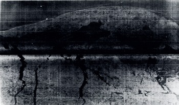
Fig. 14. SLR image of the Wainwright—Icy Cape portion of the north coast of Alaska (top of picture is south) taken 28 April 1974. The ice areas producing bright returns correspond either to ridges or rubble fields. Newly formed leads (covered with skim ice) are shown by their low return and characteristic pattern

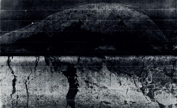
Fig. 15. SLR image of the same area shown in Figure 14 but taken three days later (1 April 1974). Note the striking change in lead configuration

Conclusion

In the above review we have tried to provide a glimpse of the usefulness of visual, passive microwave, and active microwave remote sensing techniques, as applied to studies of the geophysical aspects of lake and sea ice. The current results in this area of glaciological investigation offer a tantilizing glimpse of what can be expected to follow in the next few years when such remote-sensing data become generally available. We feel that in the very near future it will be possible to predict the dynamics and thermodynamics of the world’s sea-ice covers by a combination of numerical modeling coupled with periodic evaluations and updatings based on remote-sensing data obtained from satellite systems. Many of the pieces of the puzzle that must be assembled to accomplish this task are already available and the remaining pieces appear to be conceptually attainable. The next decade of studies of the application of remote sensing techniques for this purpose promises to be most interesting indeed.