


1 Introduction
Modeling binary outcomes—such as war, regime transitions, or policy adaption—poses considerable methodological challenges in the presence of spatial and/or temporal autocorrelation resulting from interdependent outcomes across and within units. The methodological difficulty stems from the likelihood function that involves an analytically intractable $NT$
-dimensional integral.Footnote 1
Simulation-based estimation strategies including Gibbs sampling (LeSage Reference LeSage2000) and recursive importance sampling (RIS) (Beron and Vijverberg Reference Beron, Vijverberg, Anselin, Florax and Rey2004) have been proposed to overcome this challenge. While these techniques promise to provide reliable estimates of spatial, and more recently spatio-temporal interdependence (Franzese, Hays, and Cook Reference Franzese, Hays and Cook2016), they are computationally burdensome (see Calabrese and Elkink Reference Calabrese and Elkink2014).Footnote 2
As social scientists implement research designs at increasing resolutions (e.g., at the grid-cell level) and with increasingly large datasets, simulation-based approaches quickly become infeasible.
$NT$
-dimensional integral.Footnote 1
Simulation-based estimation strategies including Gibbs sampling (LeSage Reference LeSage2000) and recursive importance sampling (RIS) (Beron and Vijverberg Reference Beron, Vijverberg, Anselin, Florax and Rey2004) have been proposed to overcome this challenge. While these techniques promise to provide reliable estimates of spatial, and more recently spatio-temporal interdependence (Franzese, Hays, and Cook Reference Franzese, Hays and Cook2016), they are computationally burdensome (see Calabrese and Elkink Reference Calabrese and Elkink2014).Footnote 2
As social scientists implement research designs at increasing resolutions (e.g., at the grid-cell level) and with increasingly large datasets, simulation-based approaches quickly become infeasible.
We provide a new estimator to address spatial, temporal, and spatio-temporal forms of interdependence embedded in binary outcome data. We build on a pseudo maximum likelihood estimator (PMLE) for binary spatially autoregressive models proposed by Smirnov (Reference Smirnov2010), and extend it to cases of temporal and spatio-temporal interdependence. So far, only Franzese, Hays, and Cook’s (Reference Franzese, Hays and Cook2016) RIS estimator has addressed the spatio-temporal case. In addition, we reduce the estimation costs by proposing an implementation strategy that avoids direct matrix inversion (of large “interdependence multipliers”), and instead relies on a combination of iterative gradient procedures and approximations that yield an estimation algorithm with almost (only) linear complexity in N.
Monte Carlo experiments demonstrate that the PMLE recovers the parameter values as good as commonly used estimation alternatives—including Bayes, GMM, RIS, and naïve probit—in a fraction of the time that simulation-based methods require. Yet, our analyses also accentuate important methodological issues that await solutions in improving the two existing estimators for spatio-temporal models (RIS and PMLE). First, both estimators generate seemingly biased standard errors. Second, we find that the performance of the RIS estimator is sensitive to the choice of data generating process (DGP). The conclusion section elaborates on these points.
2 Binary Choice Models with Spatio-Temporal Interdependence
This section specifies a binary choice model with spatio-temporal interdependence, for which we then develop a pseudo maximum likelihood estimators. We focus on the spatio-temporal case, which is applicable to cross-sectional-time-series data, noting that a purely spatial model for cross-sectional data and a purely temporal model for time-series data are nested herein. Full derivations are given in the Online Appendix.
Our analytical point of departure is a discrete-choice spatio-temporal autoregressive (STAR) model as the conventional latent variable formulation:
 $$ \begin{align} y^*_{it} = \rho \sum_{j=1}^N w_{ij,t} y^*_{jt} + \gamma y^*_{i,t-1} + \mathbf{x}_{it}\boldsymbol{\beta} + u_{it} \end{align} $$
or in matrix form:
 $$ \begin{align} \mathbf{y}^*_{(N \times T)} = \rho \mathbf{W} \mathbf{y}^* + \gamma \mathbf{T} \mathbf{y}^* + \mathbf{X}\boldsymbol{\beta} + \mathbf{u}. \end{align} $$
Here, $\mathbf {y}^{*}$
is our latent outcome variable, for which we observe realizations
$\mathbf {y}^{*}$
is our latent outcome variable, for which we observe realizations $\mathbf {y}$
, such that
$\mathbf {y}$
, such that $y_{it}=1$
if
$y_{it}=1$
if $y^*_{it}>0$
and
$y^*_{it}>0$
and $y_{it}=0$
otherwise. The spatial connectivity matrix
$y_{it}=0$
otherwise. The spatial connectivity matrix $\mathbf {W}$
captures dependency between units across space,Footnote 3
$\mathbf {W}$
captures dependency between units across space,Footnote 3 $\ \mathbf {T}$
is a temporal connectivity matrix that links the unit’s current outcomes to past realizations thereof,
$\ \mathbf {T}$
is a temporal connectivity matrix that links the unit’s current outcomes to past realizations thereof, $\mathbf {X}\boldsymbol {\beta }$
is a vector of covariates with corresponding parameters, and
$\mathbf {X}\boldsymbol {\beta }$
is a vector of covariates with corresponding parameters, and $\mathbf {u}$
is an error term (zero-mean, iid, on the individual unit level). More specifically,
$\mathbf {u}$
is an error term (zero-mean, iid, on the individual unit level). More specifically, $\mathbf {W}_{NT \times NT}$
is block-diagonal with blocks of
$\mathbf {W}_{NT \times NT}$
is block-diagonal with blocks of $\mathbf {W}^*_{N \times N}$
for each time period t, while
$\mathbf {W}^*_{N \times N}$
for each time period t, while $\mathbf {T}$
is an
$\mathbf {T}$
is an $NT \times NT$
matrix full of zeros except for the identity matrices of size N on the lower first-minor (block) diagonal. The reduced form is:
$NT \times NT$
matrix full of zeros except for the identity matrices of size N on the lower first-minor (block) diagonal. The reduced form is:
 $$ \begin{align} \mathbf{y}^* = (\mathbf{I} - \rho \mathbf{W} - \gamma \mathbf{T})^{-1} \mathbf{X}\boldsymbol{\beta} + (\mathbf{I} - \rho \mathbf{W} - \gamma \mathbf{T})^{-1}\mathbf{u}. \end{align} $$
Deriving the likelihood function requires the computation of $P(y|\boldsymbol {\beta },\rho ,\gamma ,\mathbf {X})$
, the joint probability for the observed random variable Y given the model parameters and regressors, which then requires the marginal CDF of the reduced-form error term,
$P(y|\boldsymbol {\beta },\rho ,\gamma ,\mathbf {X})$
, the joint probability for the observed random variable Y given the model parameters and regressors, which then requires the marginal CDF of the reduced-form error term, $(\mathbf {I} - \rho \mathbf {W} - \gamma \mathbf {T})^{-1}\mathbf {u}$
. This computation is analytically intractable (as long as
$(\mathbf {I} - \rho \mathbf {W} - \gamma \mathbf {T})^{-1}\mathbf {u}$
. This computation is analytically intractable (as long as $\rho \neq 0$
) due to the interdependence multiplier,
$\rho \neq 0$
) due to the interdependence multiplier, $(\mathbf {I} - \rho \mathbf {W} - \gamma \mathbf {T})^{-1}$
(Anselin Reference Anselin2002).Footnote 4
$(\mathbf {I} - \rho \mathbf {W} - \gamma \mathbf {T})^{-1}$
(Anselin Reference Anselin2002).Footnote 4
3 A PMLE for Binary Spatio-Temporal Autoregressive (STAR) Models
To circumvent this problem, we turn to a pseudo maximum likelihood method. We build on Smirnov’s (Reference Smirnov2010) spatial PMLE and extend it to cases of temporal and spatio-temporal interdependence. The remainder of the section illustrates the gist of this derivation. Here, we maintain general mathematical expressions without assuming a specific marginal distribution (e.g., logistic vs. normal). In fact, the PMLE’s feasibility regardless of the error-term distribution is one of the strengths of this approach.Footnote 5
Let $\mathbf {Z}_{NT \times NT} = (\mathbf {I} - \rho \mathbf {W} - \gamma \mathbf {T})^{-1}$
and define
$\mathbf {Z}_{NT \times NT} = (\mathbf {I} - \rho \mathbf {W} - \gamma \mathbf {T})^{-1}$
and define $\mathbf {D}$
as a corresponding diagonal matrix that contains only the diagonal elements of
$\mathbf {D}$
as a corresponding diagonal matrix that contains only the diagonal elements of $\mathbf {Z}$
, with all off-diagonal elements being zeros. This allows us to rewrite the model reduced form as:
$\mathbf {Z}$
, with all off-diagonal elements being zeros. This allows us to rewrite the model reduced form as:

Decomposing the spatial multiplier this way allows us to distinguish between zero-order and higher-order effects of an external shock as it affects observation ${it}$
. More specifically, zero-order effects capture those shocks that the unit experiences directly. Higher-order effects are spillovers of external shocks which are transmitted either spatially through other units’, or temporally across multiple time-periods. Our decomposition aggregates across both dimensions.
${it}$
. More specifically, zero-order effects capture those shocks that the unit experiences directly. Higher-order effects are spillovers of external shocks which are transmitted either spatially through other units’, or temporally across multiple time-periods. Our decomposition aggregates across both dimensions.
In order to allow for an analytical formulation of a (pseudo) likelihood, we assume that higher-order effects can be “ignored.” Behaviorally, this means that observations may simplify their choice by neglecting aggregate spatial effects of a random shock that are experienced by other (connected) observations. That is, mathematically, we do not expect a systematic effect of a random shock on unit i that is carried through the off-diagonal elements of the spatial multiplier; that is, it does not affect the choice probability systematically. The assumption is warranted because $u_{it}$
are i.i.d with mean 0. This dramatically simplifies the stochastic element of the choice probability:
$u_{it}$
are i.i.d with mean 0. This dramatically simplifies the stochastic element of the choice probability:
 $$ \begin{align} P(y_{it}=1)= P(y_{it}^* \geq 0) = F_u \left( \frac{\sum_s\sum_j \beta z_{ijs} x_{js}}{d_{it}} \right), \end{align} $$
which is now the cdf of the univariate distribution of $u_{it}$
(
$u_{it}$
( $F_u(.)$
), such as the standard normal (Probit) or a standard logistic (Logit). This allows us to write down a (pseudo) likelihood function, which is now in closed form. For any binomial link function
$F_u(.)$
), such as the standard normal (Probit) or a standard logistic (Logit). This allows us to write down a (pseudo) likelihood function, which is now in closed form. For any binomial link function $g(\cdot )$
, we have
$g(\cdot )$
, we have
 $$ \begin{align} PL(\rho, \gamma,\boldsymbol{\beta}| \mathbf{X},\mathbf{y}) \propto \prod^N_{i=1}\prod^T_{t=1} \left[ g^{-1}\left( \frac{[\mathbf{ZX}\boldsymbol{\beta}]_{ij,s}}{d_{it}} \right)^{y_{it}} \left[ 1- g^{-1}\left( \frac{[\mathbf{ZX}\boldsymbol{\beta}]_{ij,s}}{d_{it}} \right)\right]^{(1-y_{it})} \right]. \end{align} $$
Note that this expression requires an estimate for the values for $\mathbf {y}^{*}_{i0}$
, that is the values preceding the first observed period in order to calculate the first period
$\mathbf {y}^{*}_{i0}$
, that is the values preceding the first observed period in order to calculate the first period $\mathbf {y}^{*}_{i1}$
(see Equation 1).Footnote 6
Assuming mean stationarity, we draw on Kauppi and Saikkonen (Reference Kauppi and Saikkonen2008) and use what can be viewed as the unconditional expectation of
$\mathbf {y}^{*}_{i1}$
(see Equation 1).Footnote 6
Assuming mean stationarity, we draw on Kauppi and Saikkonen (Reference Kauppi and Saikkonen2008) and use what can be viewed as the unconditional expectation of $\mathbf {y}^{*}$
across all time period (and units):
$\mathbf {y}^{*}$
across all time period (and units): $E[\mathbf {y}^{*}]=(I-\rho \mathbf {W}-\gamma )^{-1} \bar {\mathbf {X}}{\beta }$
, where
$E[\mathbf {y}^{*}]=(I-\rho \mathbf {W}-\gamma )^{-1} \bar {\mathbf {X}}{\beta }$
, where $\bar {\mathbf {X}}$
are the sample means.
$\bar {\mathbf {X}}$
are the sample means.
4 Speeding Up Computation Further
Naive implementations of the proposed PMLE may still be costly to run. We further reduce the estimation costs by proposing an implementation strategy that avoids direct matrix inversion, and instead relies on a combination of iterative gradient procedures and approximations that yield an estimation algorithm with almost linear complexity in N. (Appendix 3.1 clarifies why and how.)
5 Monte Carlo Simulations
5.1 Main Results: Estimator Comparisons for the Binary Spatio-Temporal Model
We ran MCs for spatial, temporal, and spatio-temporal PMLE, comparing estimates to those of alternative estimators. Here our discussion focuses on spatio-temporal estimators. Other results are presented in the Online Appendix. The DGP is a spatio-temporal probit as specified in (1), with $u_i \sim N(0, 1)$
. We ran MCs for probit because most other existing tools are for probit models.Footnote 7
Throughout the experiments we set
$u_i \sim N(0, 1)$
. We ran MCs for probit because most other existing tools are for probit models.Footnote 7
Throughout the experiments we set $\beta _0$
to -0.5 and
$\beta _0$
to -0.5 and $\beta _1$
to 1. The covariate vector
$\beta _1$
to 1. The covariate vector $\mathbf {x}$
is drawn from the standard normal and the spatial weights matrix
$\mathbf {x}$
is drawn from the standard normal and the spatial weights matrix $\mathbf {W}$
captures queen-neighborhoods on a square lattice (row-standardized). We repeat the experiments for sample sizes of
$\mathbf {W}$
captures queen-neighborhoods on a square lattice (row-standardized). We repeat the experiments for sample sizes of $N \times T = \{64 \times 4; 64 \times 16;~ 256 \times 16 \}$
with three combinations of spatial and temporal autocorrelation:
$N \times T = \{64 \times 4; 64 \times 16;~ 256 \times 16 \}$
with three combinations of spatial and temporal autocorrelation: $\{\rho =.25~\& \gamma =.25; ~\rho =.25,~\&~\gamma =.5; ~\rho =.5~\&~\gamma =.25\}$
.
$\{\rho =.25~\& \gamma =.25; ~\rho =.25,~\&~\gamma =.5; ~\rho =.5~\&~\gamma =.25\}$
.
Table 1 summarizes the results. Overall, the PMLE recovers the parameters accurately and with reasonable precision. However, the PMLE is overconfident in some cases, suggesting that the standard errors (obtained via the Hessian) are too small. Less than one percent of runs do not converge (see Tables A7 and A8 in the Online Appendix).
Simulation results for spatio-temporal PMLE (500 iterations; $y^*_0$
is estimated by
$y^*_0$
is estimated by $E(y^*_t)$
)
$E(y^*_t)$
)

Overconfidence is the standard deviation of the estimated parameter divided by the mean of its estimated standard error.
We contend that our estimator is nevertheless useful for applied researchers. Unlike most existing spatial estimators, it can simultaneously account for both spatial and temporal autocorrelation. So far, only the RIS approach proposed by Franzese, Hays, and Cook (Reference Franzese, Hays and Cook2016) is able to estimate spatio-temporal processes for binary data. However, our PMLE is several orders of magnitude faster: on a standard PC a single run for $N\times T=64\times 16$
takes seven seconds for the PMLE, and nearly 3 h for the RIS (see Figure A3 for a summary of estimation times); for
$N\times T=64\times 16$
takes seven seconds for the PMLE, and nearly 3 h for the RIS (see Figure A3 for a summary of estimation times); for $N\times T=256\times 16$
the PMLE takes nine seconds, while we estimate the RIS to take almost two weeks if estimation time increases linearly (not executed).
$N\times T=256\times 16$
the PMLE takes nine seconds, while we estimate the RIS to take almost two weeks if estimation time increases linearly (not executed).
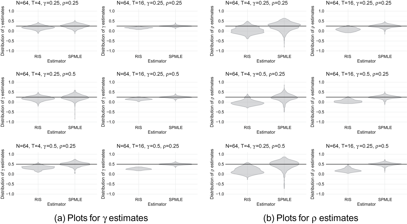
More concernedly, our experiments show that the RIS’s unbiasedness hinges on the choice of DGP, especially as true values of $\gamma $
and
$\gamma $
and $\rho $
increase (c.f. Darmofal Reference Darmofal2015, 166). For instance, the biases are not prominent under the DGPs chosen in Franzese, Hays, and Cook (Reference Franzese, Hays and Cook2016) and Calabrese and Elkink (Reference Calabrese and Elkink2014) but they are under the DGP we selected. (see Figure 1.)Footnote 8
$\rho $
increase (c.f. Darmofal Reference Darmofal2015, 166). For instance, the biases are not prominent under the DGPs chosen in Franzese, Hays, and Cook (Reference Franzese, Hays and Cook2016) and Calabrese and Elkink (Reference Calabrese and Elkink2014) but they are under the DGP we selected. (see Figure 1.)Footnote 8
Distribution of $\gamma $
and
$\gamma $
and $\rho $
estimates from Monte Carlo simulations for recursive importance sampler and pseudo-maximum-likelihood estimator.
$\rho $
estimates from Monte Carlo simulations for recursive importance sampler and pseudo-maximum-likelihood estimator.
5.2 Other Results: Estimator Comparisons for the Binary Spatial or Temporal Model
For a purely spatial DGP, we compared the Bayesian spatial probit model proposed by LeSage (Reference LeSage2000) and implemented by Wilhelm and Godinho de Matos (Reference Wilhelm and de Matos2013), a linearized spatial GMM (Klier and McMillen Reference Klier and McMillen2008), RIS (Franzese, Hays, and Cook Reference Franzese, Hays and Cook2016), a naive probit with an observed spatial lag, and our PMLE. Our experiments suggest that a Bayesian approach is preferable (see Tables A1, A5, Figure A1, and Calabrese and Elkink (Reference Calabrese and Elkink2014)). However, given its speed, PMLE potentially provides useful starting values for the Bayesian approach. Finally, we also examined a setup with just temporal autocorrelation, comparing the RIS and PMLE approach. Again the PMLE outperforms the RIS (see Tables A2, A6 and Figure A2).
6 Conclusion
In this letter, we (i) introduced an analytically tractable pseudo maximum likelihood estimator for binary choice models that exhibit interdependence across space and/or time and (ii) proposed an implementation strategy that increases computational efficiency considerably. Our Monte Carlo experiments demonstrate that the estimators are able to recover the parameters of the DGP, and requires only a fraction of the computational cost of simulation-based methods. For spatio-temporal and temporal models, the PMLE estimator outperforms the only available alternative, the RIS implementation by (Franzese, Hays, and Cook Reference Franzese, Hays and Cook2016). By contrast, for purely spatial applications the Bayesian approach by Beron and Vijverberg (Reference Beron, Vijverberg, Anselin, Florax and Rey2004) appears to perform best.
However, our PMLE approach comes with one drawback: its standard errors are potentially biased (but apparently less so than those given by the RIS). In the broader context of composite maximum likelihood approaches, Varin, Reid, and Firth (Reference Varin, Reid and Firth2011) provide an extensive review of this property. In short, the standard errors obtained via the Hessian of the PMLE tend to be underestimated for certain parameters. Generally speaking, the literature finds that the bias is greater when $NT$
is not sufficiently large compared to the variables included in the model. Our own first-cut Monte Carlo simulations (only with a single configuration of parameter values) indicate that this bias can emerge especially in the standard error estimate for the spatial parameter
$NT$
is not sufficiently large compared to the variables included in the model. Our own first-cut Monte Carlo simulations (only with a single configuration of parameter values) indicate that this bias can emerge especially in the standard error estimate for the spatial parameter $\rho $
. One approach would be a parametric bootstrap. Another approach would be an approximation, such as the use of a sandwich estimator. In this realm, for PMLEs in particular, a sandwich estimator using the Godambe information matrix appears promising (Varin, Reid, and Firth Reference Varin, Reid and Firth2011).
$\rho $
. One approach would be a parametric bootstrap. Another approach would be an approximation, such as the use of a sandwich estimator. In this realm, for PMLEs in particular, a sandwich estimator using the Godambe information matrix appears promising (Varin, Reid, and Firth Reference Varin, Reid and Firth2011).
Acknowledgments
We would like to thank Frederick Boehmke, Lars-Erik Cederman, Scott Cook, Olga V. Chyzh, Martin Elff, Jos Elkink, Robert J. Franzese Jr., Christian Kleiber, Dennis Quinn, Andrea Ruggeri, Emily Schilling, Martin Steinwand, Oliver Westerwinter, Michael Ward, Christopher Zorn as well as audiences at various conferences for their useful comments.
Data Availability Statement
The replication materials for this paper can be found at Harvard Dataverse at https://doi.org/10.7910/DVN/9SKYLD (Wucherpfennig et al. Reference Wucherpfennig, Kachi, Bormann and Hunziker2020).
Supplementary Material
To view supplementary material for this article, please visit https://dx.doi.org/10.1017/pan.2020.54.


 Open access