


Introduction
Humans like to say we crave order. We ask our children to “keep their rooms in order,” order is demanded in courtrooms, and we definitely frown on disorderly conduct. But, in fact, perfect order is perfectly boring. In the sense of regularity, it means that observing one part of something means we know all about it, and there is nothing more to learn. The painting Red Square by Kazimir Malevich (Figure 1a) is perhaps an extreme of perfect order. Intended as an avant-garde statement of the ultimate supremacy of pure feeling removed from any representational content, it does not cause the eye to linger or search for (nonexistent) details.

Figure 1: Abstract paintings: (a) Kazimir Malevich, Red Square; (b) Jackson Pollock, Number 8.
Another abstract expressionist artist, Jackson Pollock, created much more interesting paintings (Figure 1b) in which there are multiple colors and shapes. The swirls and blobs are not random, although they may appear so at first. His paintings have in fact been shown to be fractal [Reference Taylor1], one of the recurring ways that nature often organizes things. This makes Pollock's work much more interesting to view than simply a collection of randomly placed and sized paint drops in random colors (that is, complete disorder). Groupings and structures that are intermediate between perfect order and complete disorder are the most interesting. The concepts of arrangement, proportion, and pattern arise in many fields, and not just those that involve aesthetics such as flower arranging (ikebana). This is especially true in applications that include microscopy, and several are worth examining to better understand the possible types of order and the available measurement tools.
Atomic Structure
Atoms, and groups of atoms, generally form bonds that produce very regular three-dimensional arrangements. Even in liquids, there is generally some preferential local arrangement of atoms. Water, for example, has two hydrogen atoms bonded to the oxygen atom at the tetragonal angle of 104.5°, and the weak Van der Waals bonds from the dangling hydrogen atoms lead to a preferred arrangement of local molecules that is hexagonal. This accounts for the stability of the liquid, as other similar chemicals such as hydrogen sulfide are not bent, and are gases at room temperature. When water freezes, the bent molecules become lined up in the hexagonal 120° arrangement seen in snowflakes.
There are 14 Bravais lattices that are possible for long-range order. Other possibilities exist: non-periodic arrangements of regions with atomic lattices that cannot extend to fill space have been found in both man-made and natural materials (read The Second Kind of Impossible by Paul Steinhardt for a highly entertaining and scientifically sound background). It is possible using the TEM or AFM to visualize the atomic positions (Figure 2a, 2b). The bonds between atoms are very strong, and single perfect crystals have important mechanical and electronic properties, but most materials are quite imperfect. Even a 0/0/0 diamond (highest quality cut, color, and clarity) has locations in the lattice where an atom is missing (vacancy) or some atom other than carbon, for example, hydrogen, has squeezed in among the atoms (interstitial). Modern solid-state electronics depend on highly perfect silicon single crystals that are intentionally doped with atoms that replace silicon (substitution) and modify the electronic structure to create semiconductors.

Figure 2: Atomic lattices: a) TEM image of a gold nanoparticle; b) AFM image of the surface of graphite; (c) TEM image of a grain boundary in gold foil.
In addition to these local defects in crystal structure, most crystalline materials consist of multiple crystals that have different orientations. The places where these grains meet (Figure 2c) are grain boundaries that strongly affect the overall properties (and make materials orders of magnitude weaker than a perfect single crystal). In addition, dislocations within the grains are atomic-scale offsets in the regular lattice that can shift position relatively easily and so cause deformation of the grain and cumulatively of the bulk material.
Max von Laue used X-ray diffraction to reveal the periodicity of atomic spacing in crystals (for which he received the 1914 Nobel Prize in physics). Electron diffraction is commonly used to reveal the structure of specimens in the TEM and can be used to measure the atomic spacing as shown in Figure 3.

Figure 3: Measuring atomic spacings using a selected area diffraction pattern (d-spacing • radius = constant).
Many common materials, especially metals, are produced with controlled microstructures that seek to optimize the grain structure and dislocation density to provide the desired mechanical properties. Figure 4a shows the grain structure of a metal as it appears when polished and etched to reveal the grain boundaries. Generally the smaller and more uniform the grains the better the strength and ductility. Measuring the “grain size” is usually done by superimposing a circular grid and counting intersections with the boundaries, which measures the surface area of grain boundaries per unit volume [2]. This method is useful for an equilibrium grain structure, but depending on heat treatment and mechanical deformation a duplex arrangement of different populations of grains may develop, in which case the “grain size” number can be misleading. Rolling the metal to a thin sheet (Figure 4b) or drawing it into a wire squeezes the grains into a distorted shape with many more dislocations, which tangle and increase the hardness but decrease the ductility. Counting the number of intersections of a grid of lines with the boundaries as a function of direction is a commonly used method of assessing the degree of elongation and anisotropy.

Figure 4: Metal grain structures: (a) equiaxed; (b) elongated by cold-rolling.
Some macroscopic man-made objects show uniform regularity. A brick wall (Figure 5a) or hexagonal bathroom tile floor have minor variations that do not attract much attention. A parquet floor (Figure 5b) uses different wood grains and orientations that create more interest, and the elaborate tiling in the Alhambra (Figure 5c) are regular and periodic but with enough variations and symmetries to engage the viewer. Even large man-made structures often exhibit regularity and symmetry along with complexity and unique design elements. Many cities have a regular array of streets (sometimes with unimaginative names like 42nd Street and 6th Avenue), which is convenient but not interesting.

Figure 5: Macroscopic man-made objects that show uniform regularity as described in the text.
One way to measure the tendency toward regular or self-avoiding spacing and its opposite, clustering, is to measure the neighbor distances. For a random distribution, such as a view of stars in the night sky (in spite of the human desire to impose order in the form of imagined constellations), the mean nearest neighbor distance is just 0.5•(Area/Number)1/2. As illustrated in Figure 6, a self-avoiding arrangement has a greater mean neighbor distance, giving a ratio to the value for random spacing greater than 1, while a clustered one has a smaller ratio value. Fourier transforms (or diffraction spots) may also be useful if the intensity profile of the peaks can be measured to represent the variations in spacing.

Figure 6: Examples of neighbor distance with the measured ratio of mean value to the expected value for a random distribution calculated from area and number: (a) precipitate particles in a magnesium alloy (self-avoiding); (b) deposited PLGA nanoparticles (random); (c) oil droplets in an emulsion (clustered).
Partial Order
A marching column of soldiers is expected to show a perfect order with regular spacing, but in nature things are less perfect (Figure 7). Still, in a flock of birds or school of fish there is a degree of regularity that becomes apparent upon careful examination. Rather than a global regularity, each individual seeks to maintain the same approximate distances from nearby neighbors as they move in coordination.

Figure 7: Military formation vs. a flock of birds.
The characterization of partial order is important in many materials that are examined microscopically. Precipitate particles are generally self-avoiding, since their formation depletes the surrounding matrix of some element(s). Particulates that tend to cluster or agglomerate because of some attractive property, such as static electrical charge on their surfaces, may cause difficulties in application to substrates. Nonuniformity must be controlled in spraying, electrodeposition, 3D printing, painting, and even the forming of particle board. Uniformity of size and dispersal of second-phase regions in mixed polymers is important for their properties [Reference Masters3]. A molecular strategy produces self-avoidance in patterning axons and dendrites in both vertebrates and invertebrates [Reference Zipursky and Grueber4,Reference Qi and Chilkoti5]. Partial regularity characterizes the spacing of leopard spots and zebra stripes [Reference Stewart6]. Topological analysis of clusters and cluster boundaries arises in fields from astronomy to genetics [Reference Dotsenko7]. All of these, and more, are cases in which uniformity is rarely perfect but must be monitored and characterized.
Another aspect of partial order involves the need to find repetitions of a pattern that may be partially obscured or have minor variations, and may occur in non-regular positions. Cross-correlation is a useful tool for this, as illustrated in Figure 8. The process can be envisioned as sliding the target pattern over the search area and calculating the degree of match. The result shows peaks that locate and measure the degree of matches.

Figure 8: Cross-correlation analysis to identify structural patterns: (a) SEM image of a leaf surface; (b) target (enlarged to show pixels); (c) results showing peaks at matched (red) and partially matched (green) locations.
Fractal Structures
Another way that many natural structures are formed involves fractal geometry. The principle is a self-similar repetitive arrangement at many different dimensions. In erosion or turbulence, for example, processes operate in similar ways at both large and small scales. Figure 9 illustrates a strictly repetitive geometric operation that produces a Sierpinski gasket: the initial triangle has its central triangular section removed, leaving four identical smaller triangles. The same procedure is applied to each of them, and this is repeated ad infinitum leaving as an end limit a structure with an infinite boundary length and zero area.

Figure 9: Creation of a Sierpinski gasket as described in the text.
Branching structures are a common phenomenon, and these can also be created by a repetitive scaling as shown in Figure 10a. Small changes in the original pattern produce different results [Reference Prusinkiewicz and Lindenmayer8]. Using several structural elements with associated probabilities of occurrence produces a family of recognizably related but individual forms (Figure 10b). It requires very few rules, which can be compactly encoded genetically, to distinguish maple trees from oaks, for example. Figure 11a shows tree-like branching with characteristic angles defined by atomic structure in growth of dendritic crystals. Fractal dendritic crystal growth is a problem that results in shorting of rechargeable batteries, but it also produces the infinite variations of snow crystals.

Figure 10: Iterating a branching shape forms a tree: (a) varying the rules alters the resulting tree shape; (b) using probabilities for different branch patterns produces a family of different but recognizably related forms.

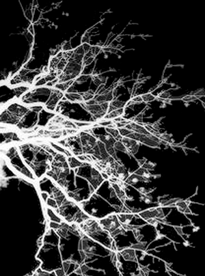
Figure 11: Natural branching shapes: (a) growth of copper dendrites; (b) neurons in the brain; (c) 3D reconstruction of airways in the human lung.
Figure 11 also shows the branching patterns in neurons and in the airways in the human lung. Many anatomical structures, such as the human vascular system, are fractal, and differences in the dimensions often distinguish healthy from abnormal conditions [Reference Goldberger9]. A fractional dimension for these branching patterns relates the total measured length to the resolution of ever-smaller branches or tributaries. A cumulative log-log plot of total length as a function of the length of included skeleton branches provides a measure of the fractal dimension.
When Mandelbrot [Reference Mandelbrot10] introduced the term “fractal” to describe structures that have more and more detail present at ever finer scales, one example was the length of the coast of Britain. Plotting the measured length as a function of the ruler used for measurement [Reference Richardson11] produces a straight line plot on log-log scales, whose slope gives the fractional dimension. There are more convenient ways to determine the dimension, one of which is shown in Figure 12 using the coastline of Australia. Measuring the area of a ribbon centered on the coast as a function of the ribbon width is quickly done by plotting the cumulative values in the Euclidean distance map, which assigns each pixel in the image a value representing its distance from the edge. Similar measurements show, for example, that the Hawaiian Islands generally have an increase in fractal dimension with age, with the youngest being the smoothest [Reference Russ12].

Figure 12: Measuring the fractal dimension of Australia based on the Euclidean distance map.
Measurement of the border of tumors shows that higher fractal dimension indicates a greater likelihood of malignancy. The fractal dimension of surfaces arising from some types of fracture or wear correlates with the energy absorbed in the process [Reference Srinivasan13]. Wear on archaic stone tools produces fractal surfaces that indicate the use of the tool (scraping, cutting, etc.). Surface fractal dimension determines how well surface contacts can transmit heat or electricity [Reference Hyun14]. Figure 13 shows SEM images of fractal surfaces in 3 dimensions formed by erosion and by growth.

Figure 13: SEM images of 3D fractal structures: (a) sponge; (b) weathered granite.
Fiber Arrangements in Two and Three Dimensions
One very important field where random, self-avoiding, and highly regular arrangements are used for their contribution to specific properties is in textiles, both woven and nonwoven. Materials constructed of fibers are often thin and essentially two-dimensional, such as cloth and paper, and may have a high degree of order, be partially ordered, or be highly disordered. The simplest form of woven cloth consists of orthogonal fibers; the interlacing of these fibers usually follows one of several common weave patterns (Figure 14). The intermixing of different colored threads introduces patterns in the cloth, and advanced techniques, such as Jacquard weaving that combine multiple patterns and colors, can produce extremely complex designs. Basic weaving has been performed by humans for at least 8,000 years.

Figure 14: Some common regular weave patterns, with horizontal weft and vertical warp: (a) plain; (b) basket; (c) twill; (d) herringbone.
As shown in Figure 15, fibers oriented in different directions, either by design or accident, may introduce more irregularity to the pattern. Woven fabrics may have complex patterns but are still primarily regular with repetitious structural arrangement. Nonwoven materials are assuming increasing importance because of their properties. Nonwovens such as paper may have partial isotropy, substantial anisotropy, or approach randomness. It is important to understand that extreme anisotropy may not produce randomness in local areas. Arrangements, even locally, in which fibers are predominantly aligned may produce higher density (lower permeability and porosity) and weaker transverse strength. Fiber orientation, determined using analysis of images from light or electron microscopy in 2D or microCT in 3D can provide measurements of local fiber orientations, which are typically represented by polar plots of the orientation distribution function.

Figure 15: Arrangements of fibers: (a) regular orthogonal weave; (b) irregular orthogonal weave; (c) regular weave including variations in angle; (d) irregular predominantly orthogonal weave; (e) partially aligned bonded nylon fibers; (f) nonwoven “random” fibers in paper.
In three dimensions things become more complicated. Even if the third (thickness) dimension is relatively small compared to lateral extent, the orientation of fibers can vary greatly and this strongly affects properties such as permeability (for example, filters). A fully 3D arrangement of “randomized” fibers (Figure 16) generally shows strong preferred orientations and cannot achieve high density because the fibers interfere with each other. With either straight or flexible fibers, this increases pore space and fluid retention, important for absorption of fluids (for example, diapers).

Figure 16: A partially “randomized” 3D array of straight fibers with its orientation distribution function showing the degree of partial order.
Randomness may be treated as either a particular form of order or the absence of order. Questions of randomness are very difficult to answer [Reference Martin-Löf15]. For example, biochemists have puzzled whether proteins are the result of historic stepwise construction or are random sequences of individual peptides that have been selected by evolution. Intuition often fails in attempting to define or detect true randomness in a sequence, although at any point it may be impossible to predict the next value [Reference Delahaye and Dubucs16]. Statistical analysis shows that each of the digits in the value of pi (3.1415926…) has the same overall frequency of occurrence, but there is no pattern of regularity, repeats, or order in the sequence. Yet it can hardly be called random since it is entirely determined by a simple mathematical constant.
Conclusion
There are a variety of methods that can be used to characterize the regularity of patterns, including diffraction and various measurement techniques. These are applicable at any scale, from atomic to real-world dimensions. As arrangements depart from perfect order, the measurements that can meaningfully describe them become increasingly difficult and vary from one application to another. Finally, determining that a pattern is truly random is extremely difficult; the statistical tests required are complex and not very satisfying. Relying on human vision to assess a degree of order or randomness is generally insufficient.


