

A fundamental challenge for any governing system is to elect representatives who accurately represent their electorates. In order to meet this challenge, democracies have often engaged in “electoral engineering:” making choices about their basic electoral system (Norris Reference Norris2004), shifting the way that legislative districts are drawn (Cain Reference Cain1984; Winburn Reference Winburn2008), making alterations to the way that ballots are cast (Engstrom and Kernell Reference Engstrom and Kernell2005), imposing limits on terms (Carey Reference Carey1998), and modifying the formal role of parties (Argersinger Reference Argersinger1980; Masket Reference Masket2007). Can electoral engineering lead to improved representation?
The state of California engaged in a grand experiment of electoral engineering in 2012, implementing two major reforms. All legislative districts were drawn by California’s first-in-the-nation Citizens’ Redistricting Commission, whose members were selected by lot rather than appointed. The primary elections were also the contested under new “top-two” rules—which opened them to all voters and advanced the top-two candidates to November, regardless of party. Did these reforms succeed in improving representation?
In this paper, we propose a novel method for gauging the match between the policy preferences of the median voter in every district and the position of the legislator representing this district. There is, of course, a long and important literature on the impacts of reforms to primary election rules and of redistricting processes. Scholars have measured, separately, their effects on voter behavior, district characteristics, or legislative roll calls. For instance, they have studied the impact of redistricting institutions on the competitiveness of districts (Kogan and McGhee Reference Kogan and McGhee2012) as well as the effect of primary election rules on the representativeness of electorates (Marshall Reference Marshall1978; Kaufmann, Gimpel and Hoffman Reference Kaufmann, Gimpel and Hoffman2003), on crossover voting and voter turnout (Alvarez and Nagler Reference Alvarez and Nagler2002; Gaines and Cho Reference Gaines and Cho2002; Sides, Cohen and Citrin Reference Sides, Cohen and Citrin2002), on moderation versus extremism among legislators (Gerber and Morton Reference Gerber and Morton1998; McGhee Reference McGhee2008; Bullock and Clinton Reference Bullock and Clinton2011; Ahler, Citrin and Lenz Reference Ahler, Citrin and Lenzforthcoming), and on each lawmaker’s centrality to the voting network of legislators (Alvarez and Sinclair Reference Alvarez and Sinclair2012). Yet, past studies have not looked at voters in combination with the lawmakers representing their districts to see whether politicians deliver what their constituents want. Our project combines data on voters and politicians to see whether California’s reforms led to a closer congruence between the average voter’s policy preference and the legislator’s policy positions in each district.
Measuring the quality of representation has long been a challenge for political scientists, as we discuss in the next section. One normative ideal is that the quality of a representation is inversely proportional to the distance between a district’s median voter and its elected representative (Downs Reference Downs1957). The empirical difficulty comes, as we explain in the next section, in measuring both of these positions on a common scale. Yet, two recent methodological advances in the study of politics allow us to evaluate the congruence between voters and legislators across districts and time.
The first advance comes in the ability to locate voters and legislators in the same ideological spectrum, by observing their responses to a common set of policy questions. The second advance has come in the multilevel regression and post-stratification (MRP) method, which allows to use a single statewide survey to predict the position of the average voter in every district, across multiple elections. This combination could be replicated at a reasonably low cost in other political settings to help evaluate the causes and consequences of congruence in legislative representation.
Our research combines these methods to evaluate the success of California’s democratic engineering. Our methodological contribution comes in showing how to perform this combination, and providing evidence that it produces reliable data that unlocks the door to new substantive questions. First, we conduct a poll asking Californians a set of 46 policy questions previously asked of California House candidates. Then we jointly scale these responses in order to create a comparable common ideological space. Next, we use the MRP technique along with Census-derived district demographics to estimate the position of the average voter in every district in both the 2010 (pre-reform) and the 2012 (post-reform) elections. By comparing the congruence of voter positions with legislator positions before and after the implementation of the new primary and redistricting rules, we can assess whether these reforms improved representation in the state’s assembly, senate, and congressional delegation. In an analysis that focuses on California’s congressional delegation, we find no evidence that reform improved representation. If anything, California’s congressional candidates and eventual lawmakers became a bit more ideologically extreme in 2012, thus moving further apart from the average voter in their district. We evaluate other hopes of reformers (that more competitive districts will yield improved representation) and again do not find clear support.
Measuring Representation
Because “the history of political theory is studded with definitions of representation” (Eulau et al. Reference Eulau, Wahlke, Buchanan and Ferguson1959, 742; see also Pitkin Reference Pitkin1967; Mansbridge Reference Mansbridge2003), empirical work must focus on one concept in order to move toward a functional measure. Eulau and Karps (Reference Eulau and Karps1977) outline four types of description that legislators can provide: policy responsiveness, constituent service, pork-barrel allocations, and descriptive representation. We take the first of these as our focus. Beginning with Miller and Stokes (Reference Miller and Stokes1963), scholars have probed policy responsiveness by asking whether the issue positions of legislators match up with those of their constituents. This “quickly became the default definition of representation” (Grimmer Reference Grimmer2010, 9) and has been the focus of much influential scholarship (Achen Reference Achen1978; Poole and Rosenthal Reference Poole and Rosenthal1997; Clinton Reference Clinton2006).
Even with conceptual clarity, comparing the quality of policy representation provided before and after a reform, or from one political system to another, presents an empirical challenge. Scholars often have information about the political ideology of voters in particular districts, states, or nations, and can use it as an explanatory factor in a regression explaining the policy positions of representatives or governments. A positive relationship between voter ideology and elite positions does indeed indicate that constituents have been provided with some level of policy of representation; more liberal voters receive more liberal representation. Yet, to go one step further—to argue that one political system or set of rules produces better representation than another—requires that the positions of both voters and politicians be measured on the same scale.
Why? Without a common scale, comparing the slopes of the link between voter ideology and elite positions between two different systems cannot tell us which system performs better. A steeper slope, sometimes taken as evidence of “tighter representation,” might in fact be evidence of a looser link between voter and elite positions. How should elites respond to a one-unit increase in voter ideology? If voters and elites are not measured on the same scale, the correct response bringing elites into line with voter positions might be a half-unit increase, a one-unit rise, or a two-unit increase; it all depends on the scale of the two measures.
We are not original in making this point. Erikson, Wright and McIver (Reference Erikson, Wright and McIver1993) make it, explaining that this prevents them from comparing the representativeness of sets of states with different institutional features. Matsusaka (Reference Matsusaka2001) bases a convincing critique upon it. Yet, our work comes at a time when advances in the joint scaling of voter and elite preferences, along with the estimation of voter positions across many political units, allow a new solution to this old problem in the study of representation. In this section, we describe both of these advances and how we combine them to compare levels of representation.
Locating Voters and Lawmakers on a Joint Ideological Scale
Comparing representation requires, as a first step, measuring the policy positions of both lawmakers and voters and then placing them on the same ideological scale. In the modern era of quantitative studies, scholars have been able to locate elected officials on an ideological spectrum based on the ratings that they receive from interest groups (Poole and Rosenthal Reference Poole and Rosenthal1984), the survey responses they give in election campaigns (Ansolabehere, Snyder and Stewart Reference Ansolabehere, Snyder and Stewart2001), and the roll-call votes that they cast on a legislative floor (Poole and Rosenthal Reference Poole and Rosenthal1997). While ideal point estimation techniques have been dominated by congressional applications, newer work finds applications in California (Masket Reference Masket2007) and state legislatures more broadly (Cox, Kousser and McCubbins Reference Cox, Kousser and McCubbins2010; Shor and McCarty Reference Shor and McCarty2011). On the other hand, for a half-century, researchers have gauged the ideological orientations of voters by asking them to identify as liberal or conservative on some scale. This measure is notoriously noisy and crude. Achen (Reference Achen1975) and Ansolabehere, Rodden and Snyder (Reference Ansolabehere, Rodden and Snyder2008) conceptualize the problem of determining individual ideology from the perspective of measurement error. This perspective suggests alternatives to abstract single-item questions about ideology such as multi-item issue preference scores that evince far greater individual stability than self-reported ideology. Ansolabehere, Rodden and Snyder (Reference Ansolabehere, Rodden and Snyder2008) also show that these scales approach the stability of party identification in applications like vote choice.
Yet, even if we had perfect measures of individual ideology, it would not be enough to properly assess congruence in representation. The key is bridging across different political institutions and contexts. Examples include joint estimates of ideology for the US House and Senate (Poole Reference Poole1998; Groseclose, Levitt and Snyder Reference Groseclose, Levitt and Snyder1999), or for presidents and Congress (McCarty and Poole Reference McCarty and Poole1995), and state legislators and Congress (Shor, Berry and McCarty Reference Shor, Berry and McCarty2010; Shor and McCarty Reference Shor and McCarty2011). Scales are identified by the analyst’s assumptions about the consistency of behavior when a bridge actor moves from one setting to another. Another approach to bridging ideal points across institutions is to see how actors in each group respond to a common set of questions. When legislators and survey respondents are asked to weigh in on exactly the same issues, we can see how they line up on the same ideological scale.
Recent works have revived the interest, which dates back to Miller and Stokes (Reference Miller and Stokes1963) and Achen (Reference Achen1978), in linking voters to their representatives. Some approaches rely on survey respondents’ perceptions of candidate ideology (Erikson and Romero Reference Erikson and Romero1990; Alvarez and Nagler Reference Alvarez and Nagler1995; Merrill and Grofman Reference Merrill and Grofman1999), though these data may be systematically biased (Conover and Feldman Reference Conover and Feldman1982). A growing literature characterizes a common ideological space for citizens and legislators (Gerber and Lewis Reference Gerber and Lewis2004; Bafumi and Herron Reference Bafumi and Herron2010; Stone and Simas Reference Stone and Simas2010; Buttice and Stone Reference Buttice and Stone2012; Warshaw and Rodden Reference Warshaw and Rodden2012), or incumbents and challengers (Bonica Reference Bonica2014). Jessee (Jessee Reference Jessee2009; Jessee Reference Jessee2010; Jessee Reference Jessee2012) links together citizen preferences with the publicly announced positions of presidential candidates in a common ideological space.
Each of these approaches is an advance and yields data appropriate for each authors’ particular research question. For the purposes of comparing representation, though, we need an approach that gives us common space ideological estimates for large numbers of survey respondents, estimates for incumbents, and estimates for challengers. Works by Shor and Rogowski (Reference Shor and Rogowski2016) and Shor (Reference Shor2014) provide this, measuring the ideology of a sample of voters and of political winners and losers alike on a common scale by comparing their answers to the same comprehensive set of policy questions. We adopt this approach by conducting a California poll and asking survey respondents questions drawn from Project Vote Smart’s “National Political Awareness Test,” which provides a clear public record of where candidates stand on a range of issues. These surveys of candidates ask candidates to take explicit support or oppose positions on a wide range of both economic and social policy questions. Because a single, national organization poses the same questions to all candidates, this source provides a more comprehensive catalog of campaign positions than candidate advertisements, local debates, or press coverage can. Because the organization’s goal is to make each politician’s positions clear so that voters can compare themselves with candidates on the ideological spectrum, there is a clear fit between the process that generates these data and the use that we make of them.
We conducted a statewide poll of a random sample of 1000 California registered voters in the two weeks leading up to the June 2012 primary. This poll, administered online by the firm YouGov, asked voters a series of 46 Yes/No questions about their policy preferences, grouped by issue area. These questions, which are reported in our Online Appendix, were drawn from Project Vote Smart’s survey of candidates for state legislative and congressional office. For the 2010 election, we also supplement the National Political Awareness Test (NPAT) survey responses with candidate positions noted by Vote Smart’s VoteEasy tool. The organization researched answers to a subset of the NPAT survey even for candidates who did not fill out their own surveys.Footnote 1
This provides us with data on the issue positions of 172 House candidates in the 2010 and 2012 elections,Footnote 2 enabling us to look at the electoral connection between legislators and voters in the vast majority of California districts. The positions of both voters and politicians generally fall along a single ideological dimension.Footnote 3
Estimating Voter Positions Across Many Legislative Districts
Measuring and placing voters’ and lawmakers’ ideologies on the same scale is the first step toward quantifying representation. However, in order to see whether a particular legislator shares the ideological position of the typical, or “median,” voter whom she represents we need to also generate estimates of district-level ideology, and to do so for both 2010 and 2012. Since it would be prohibitively expensive to conduct a separate survey in each of California’s 53 congressional districts, as well as its 120 legislative districts, we need to be able to generate opinion estimates from a single statewide poll (the same poll we used to link voter and lawmaker ideology).
Fortunately, a technique exists for doing this—multilevel regression and post-stratification (MRP). MRP was first developed by Gelman and Little (Reference Gelman and Little1997) and Park, Gelman and Bafumi (Reference Park, Gelman and Bafumi2004), and popularized by Lax and Phillips (Reference Lax and Phillips2009a; Lax and Phillips Reference Lax and Phillips2012). Existing work shows that, when properly implemented, MRP can use as little as a single opinion poll and a relatively simple demographic–geographic model of individual opinion to produce highly accurate estimates of voter preferences by state, congressional district, and even state legislative districts (Lax and Phillips Reference Lax and Phillips2009b; Warshaw and Rodden Reference Warshaw and Rodden2012).
MRP proceeds in two stages. In the first, individual survey responses and regression analysis are used to estimate the opinions of different types of people. A respondent’s opinions are treated as being, in part, a function of his or her demographic and geographic characteristics. Research has consistently demonstrated that demographic variables are crucial determinants of individuals’ political opinions, particularly their ideological orientation. In addition to demography, survey responses are treated as a function of a respondent’s geographic characteristics. Why are geographic predictors included? Existing research has shown that place in which people live (e.g., state, region, etc.) is an important predictor of their core political attitudes (Erikson, Wright and McIver Reference Erikson, Wright and McIver1993). Lax and Phillips (Reference Lax and Phillips2009a) demonstrate that the inclusion of geographic predictors greatly enhances the accuracy of MRP opinion estimates when compared with models that rely exclusive on demographic predictors.
The second stage of MRP is referred to as post-stratification. Based on data from the US Census, we know what proportion of a given district’s population is comprised by each demographic–geographic type from stage one. Within each district, we simply take the estimated ideology across every demographic–geographic type, and weight it by its frequency in the population. Finally, these weighted estimates are summed in each district to get a measure of overall district-level ideology (i.e., the ideology of the “mean voter”).
Using MRP, we generate estimates of mean voter ideology in every district for both 2010 and 2012.Footnote 4 These estimates are generated using our YouGov poll, conducted during the spring of 2012. Using this single poll is fine as long as we can safely assume that the relationships between demographics, geography, and ideology have not changed dramatically among voters over the two years and that respondent ideology does not fluctuate much over the same period. We know the 2010 and 2012 congressional district for each respondent in our poll, which allows us to estimate the appropriate district effect.
We begin with the comparison with a measure of district ideology developed by Tausanovitch and Warshaw (Reference Tausanovitch and Warshaw2013). These authors measure the ideology of all national congressional districts prior to the 2012 redistricting by pooling responses from a variety of surveys over a decade. In their analysis, the number of respondents per congressional district averaged 600 (many more than we have per district). The correlations between their measure and ours is 0.93. Presidential vote is another proxy measure for district ideology. When we correlate our measures of ideology to presidential vote in congressional district, we receive similarly positive evidence. The correlation between our measures of district ideology and the 2008 and 2012 Obama vote is 0.99 and 0.97, respectively. Judged against two benchmarks, it appears that our survey and methodology produce an accurate and valid estimate of voter preferences. We use our measure in the remaining analysis, rather than these alternative approaches, for two reasons. First, we can use it in all types of districts and in years both before and after California’s reforms, instead of being constrained to looking at congressional districts before redistricting. Second, it is based on policy questions rather than political choices, and places voters on the same ideological scale as legislative candidates.
In sum, our methodological contribution here is to show that a novel combination of two recent innovations—MRP and joint scaling—produces valid measures that allow us to address the fundamental question of legislative representation. By designing a poll that asks voters the same policy questions as politicians, while recording the legislative districts in which they live, we can use MRP to place not just individuals but also their districts on a joint scale with the politicians who represent them.
California’s 2012 Reforms
In 2008, voters created the Citizens Redistricting Commission to draw state legislative lines through the passage of Proposition 11, and then expanded its authority to congressional districts in 2010. The Commission was made up of 14 registered voters selected through a complex process of application, screening, and random selection, and given the authority—previously reserved to legislators and the governor—to craft new district lines after the 2010 Census. That year, voters also approved Proposition 14’s creation of the top-two primary, in which any voter could back any candidate in the spring election, with the top-two vote-getters, regardless of party, advancing to November’s general election. Each reform first went into effect in 2012.
Both were sold as antidotes to the failures of representation that had increased partisan polarization over the past decade. Yet, each was designed to fix the system through a different mechanism, in different types of districts. Reformers hoped that the new redistricting commission would draw many more districts that were competitive in November. Because the new primary rules would often deliver two members of the same party into general elections, voters from both parties and independents could band together to elect the candidate positioned closest to the median voter. In the next sections, we set out the intended impacts of the two reforms and develop concrete hypotheses about the empirical patterns that they should, if successful, create. Specifying these divergent effects is crucial, of course, because they were implemented simultaneously between the 2010 and 2012 elections.
But it is also important to note, for the purposes of our research design, that little else changed in California politics between these two contests. While much of the nation saw a “red surge” that gave Republicans control of Congress, California instead witnessed a “blue riptide” in which Democrats increased their control of the state legislature and won the governorship and a US Senate race by double-digit margins. California’s electorate became notably more diverse in 2010, with Latino voters composing 23 percent of the electorate. In 2012, these trends continued, with Democrats again picking up state legislative seats, with the state’s electorate continuing to grow more diverse, and with President Obama carrying the state in a landslide at the top of the ticket.
With overall political conditions quite similar in 2010 and 2012, California provides a strong interrupted time series research design in which we can study the two major rule changes by comparing representation before and after their implementation. We lay out the expectations that reformers had for their impact below.
The authors of Proposition 11 had many hopes for the Citizens Redistricting Commission (Kogan and McGhee Reference Kogan and McGhee2012). To improve political representation, the key goal was that by drawing many competitive districts that both parties had the chance to win, Commissioners would construct the sorts of contests in which a real electoral threat pushed candidates to match the positions of the average voter. The ballot argument in favor of Proposition 11, as well as the statements of its supporters, made the explicit case that the new process would lead to more representative districts. “If Legislators don’t have to compete to get re-elected, they have no accountability to voters,” the initiative’s proponents argued.
Before the new districts got their first run in the 2012 elections, voters changed another important electoral rule. The top-two primary radically revised the rules of primaries with the aim of creating new general election winners. Under the new rules, voters from any party or without a party affiliation can support any candidate in the primary. With the primary electorate now a microcosm of the full district, candidates located closer to the district median could actually stand a chance in the primary. When the top-two primary candidates, regardless of party, advanced to the November runoff, it would be possible for a more moderate member of the district’s dominant party to win by appealing to a coalition of voters in her own party, independents, and in the opposition party centered around the district’s ideological median.
Backers of Proposition 14 were clear about these intentions, and they promised that this dynamic would work all across the state, not just in the competitive districts that the Citizens Redistricting Commission would create. The Los Angeles Times reported that, “Even in districts gerrymandered to favor one party, proponents of the constitutional amendment say, it would give independent voters and those in the non-dominant parties some say in who will represent them.”Footnote 5
Empirical Predictions About the Impact of the Reforms
The predictions of reform groups produce a set of clear empirical predictions about how legislative representation should change in California from 2010 to 2012. We illustrate the hoped-for effects of each reform through the reasoning of spatial voting, often used by political scientists to predict where candidates will position themselves and who will win based on the ideological distribution of voters (Downs Reference Downs1957). Following more formal spatial models, our illustrative tool makes a set of simplifying assumptions that do not always perfectly reflect reality: voters chose the candidate who is closest to them on the ideological spectrum, they have the knowledge to identify that candidate, there is some barrier to entry that prevents an unlimited number of candidates, and a candidate takes a position that remains constant from the primary through the general election. If these assumptions are met, consider who wins in under the rules and political conditions that prevailed across California in 2010. This is the district depicted in Figure 4(a), a district safely held by one party with semi-closed primary rules making the spring contest a fight mostly within the dominant party. Our hypothetical district resembles the 23rd Congressional District, where Democrats held a 47–28 percent registration edge over Republicans. (As a result of a bipartisan gerrymander, one party or the other held a substantial edge in nearly every district in 2010.) The density curves in our figure show how each party’s voters would be distributed across the ideological spectrum, based on the mean party positions and spread within each party that we found in our statewide sample. In the primary, a candidate taking a position that matched the Democratic Party’s median voter in the district would win by attracting the most votes within that party. Republican voters would follow suit by nominating a candidate in line with their party’s median voter, who would then lose in the general election as the Democrat rode her party’s registration edge to victory. The winning lawmaker, then, would be a good distance from the district’s median voter.
This ideological gap between the winner and median voter should shrink under the top-two primary, its proponents claim. Even in districts in which one party possesses a strong edge in partisan registration, as we see in the first district depicted in Figure 4(b), the new rules allowing voters from any party along with those who state “No Party Preference” to take part in the primary should advantage candidates who appeal to more than just the largest party’s base. This is illustrated by the fact that the electorate is a single, three-peaked distribution of voters rather than three separate groups of voters. With a broader distribution of voters now in play, primary contestants could pursue a number of different strategies. The exact location of the top-two vote-getters would depend on how many candidates entered the contest and where they emerged, but a likely scenario is that one would succeed by positioning herself at the dominant party’s median and the other, often a member of the same party, would make it through to November by taking a stance nearer the district median, winning votes from independents and members of the other party. The general election would be a true contest, with the advantage held by the candidate positioned closest to the middle of the district. Even in a deeply blue or deeply red district, then, the top-two rules should lead to better representation:
Hypothesis 1: Even in a district safely held by one party, congruence between the district’s median voter and the general election winner should be higher when top-two rules are in place.
Hypothesis 2: If two candidates from the dominant party advance out of the primary in a safe district, the candidate closest to the district’s median voter should win in the general election.
If the Citizens Redistricting Commission brings better representation to California, its effects should be concentrated in the most competitive districts, where legislators are forced to fight for votes. As Kogan and McGhee (Reference Kogan and McGhee2012) shows, the Commission-drawn districts created several “highly competitive” districts (six in the state assembly, three in the state senate, and four in the US House delegation) in 2012. After a decade that saw few closely matched districts, the new lines introduced the sort of swing district, contested under top-two primary rules, that is depicted in the second district in Figure 1. Notice that in a district that is more evenly balanced between the major parties, the heights of the curves representing each party’s voters are the same height. Winning the dominant party’s primary is no longer tantamount to victory, forcing candidates to look ahead to the general election by taking positions attractive to independent voters. The ultimate winner will be the one located closest to the district median.
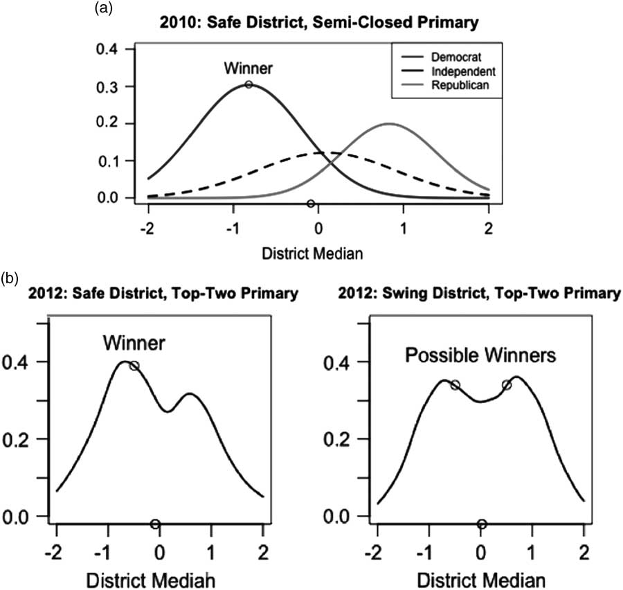
Fig. 1 Spatial voting illustration (a) Before reform (b) After reform
If this logic plays out in California elections, legislative representation should improve in politically contested territory. The Commission’s work might not change politics in solidly blue areas such as San Francisco or Los Angeles’ liberal Westside, or in steadfastly red areas in the Central Valley or southern Orange County. But in new battleground districts drawn in places like the Inland Empire, the Bay Area exurbs, Sacramento, the border between Los Angeles and Orange Counties, and Ventura, politics should change. The Democratic and Republican Parties will face a clear incentive to run more moderate candidates for office in these marginal territories, and the winner should be the one most tuned in to voter needs. This leads to two clear hypotheses about the impact of the Citizens Redistricting Commission implemented along with the top-two rules:
Hypothesis 3 : Congruence between the district’s median voter and the general election winner is higher in a competitive district than in one dominated by one of the parties.
Hypothesis 4: By creating more competitive districts, the Citizens Redistricting Commission’s plans improved legislator–voter congruence in 2012.
Of course, there was the possibility that California’s election would not unfold exactly as reformers intended. There were reasons to be skeptical of whether the new districts and primary rules would deliver on their promise, reasons that can be phrased as flaws in the assumptions that underlie the spatial voting logic. In order for either reform to work, voters need to be able to discern the ideological positions of candidates and to support those closest to them. In these down-ballot legislative contests, sorting out a moderate Democrat from a liberal one can be quite difficult, and Ahler, Citrin and Lenz (Reference Ahler, Citrin and Lenz2016) find that voters in fact had great difficulty doing so. Incumbents who had taken extremist positions to win under the past rules may be tethered to those positions but still electorally powerful, weakening the impact of the reforms at least in the short run.
Hypothesis 5 : In all types of districts, voter–legislator congruence remained constant or even declined after the implementation of redistricting and top-two reform.
The Impact of Reform on Legislative Representation
Before testing these hypotheses, we present descriptive figures and analyses confirming that our measures of voter and candidate ideology fit with expectations about California politics, and that there is some spatial content to voting in these elections. The bottom plot in figure 2 draws on our statewide random sample of registered voters to chart their positions, based on responses to the same set of 46 Vote Smart issue position questions. Based on their survey responses, voters from the two major parties occupy their expected places in the ideological spectrum, with independents centered almost perfectly in the middle. Unsurprisingly, there is little crossover between the curve representing Democratic and Republican registrants, indicating that there are only a few moderates in either party who occupy the same centrist ideological ground inhabited by the other party’s moderates. There are independentsFootnote 6 located in the middle of the spectrum, a group that now composes 26.9 percent of California’s electorate.
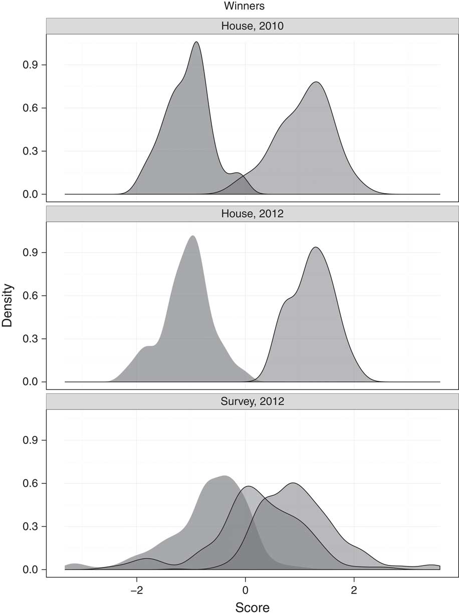
Fig. 2 Ideological positions of California’s voters (bottom) and US House Representatives by party, 2010–2012
Figure 2 also reports the ideological distributions of elected officials from both parties, allowing us to compare voters with lawmakers. The top-two panels report the positions of all lawmakers elected to the US House in the 2010 and 2012 elections, while the bottom panel summarizes survey respondents’ ideology by self-identified partisan status. First, notice that there is no non-major party shaded region for the lawmakers, because not a single member of California’s congressional delegation was elected as an independent or minor party member.Footnote 7 Note, too, that Independent voters in the middle of the ideological spectrum have little representation. Neither do either major party’s more centrist voters, because elected officials from both parties are more polarized than California voters. The median Democratic lawmaker is located far to the left of the typical Democratic voter, just as the median Republican legislator is to the right of that party’s base.Footnote 8 Moderates in either party are a scarce breed, leaving the middle of the ideological spectrum virtually uninhabited, providing no representatives to match the policy preferences of voters in the middle. It is this democratic disconnect—precisely measured in Figure 2, but long bemoaned by observers of California politics—that inspired the reforms that reshaped California elections.
Figure 2 also provides initial evidence that the reforms of 2012 did not resolve this disconnect. Drawing on evidence from all winning congressional candidates, it compares the ideological distribution of candidates in pre-reform 2010 to post-reform 2012. If the reforms shifted legislators back to the center of the political spectrum, the distributions representing their 2012 positions should be closer to the middle. Instead, we see that lawmakers shifted marginally to the extremes, particularly in the Republican Party (where many of the party’s remaining moderates lost in 2012). At least judged by candidate positions in campaigns, the new rules did not bring the return to moderation that many of their backers had expected.Footnote 9
Now we proceed from a survey-level analysis comparing voters and candidates with the district level, using the MRP procedure described above. Figure 3 shows the major party candidates and district means for the 53 districts in California for the post-reform (2012) elections (a similar figure for pre-reform elections, not displayed here, shows similar patterns). Districts are ordered by the ideological position of their mean voter, with the most left-leaning districts at the top and the most right-leaning on the bottom. Two things are immediately obvious. First, district means are generally fairly centrist throughout California; on the other hand, candidates are generally polarized and divergent. Next, the extent of that polarization has little to do with the position of the average voter in each district. While left-leaning districts tend to elect Democrats, there are moderate Democrats in some of the most liberal districts leaning districts tend to elect Democrats, as well as liberals in some of the most moderate districts (such as Julia Brownley in a more affluent coastal seat). There is a large jump in ideology between the most conservative Democrat and the most liberal Republican, but within each party, ideological positions and thus the level of polarization are not a clear function of district ideology, either in 2010 or 2012.
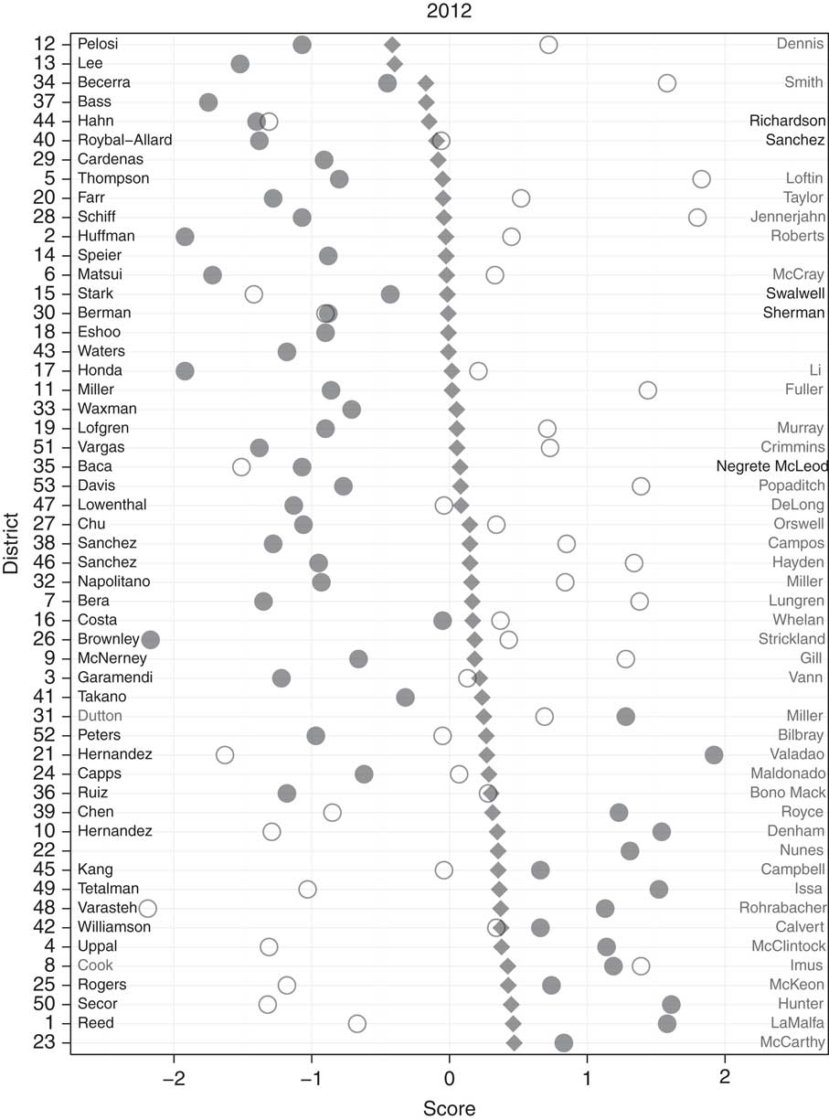
Fig. 3 2012 Voter–candidate congruence, by Congressional district Note: Circles on the left represent the positions of Democratic candidates, circles on the right are Republican candidates, and winning candidates have filled circles. In cases of a same-party contest, the leftmost candidate ideologically is on the left hand side of the figure, and the rightmost candidate ideologically is on the right hand side of the figure. Gray diamonds indicate the position of the mean voter in each district.
District ideology also does not appear to predict congruence with the mean voter, with lawmakers like Becerra and Eric Swalwell (Bay Area) matching the average voter in liberal districts and Jim Costa (Central Valley) and George Takano (Inland Empire) providing congruent representation in more moderate districts. This is evidence against Hypotheses 3 and 4: the competitive, moderate districts drawn by the Citizens Commission do not seem to lead to the election of representatives who are systematically closer to the average voter (a pattern we later confirm by showing the lack of a correlation between competitiveness and representation across all districts).
What this figure does not show is who performed best in these contests, the candidate closest to the district median or the one farther away. Table 1 answers this question, providing evidence that there is some spatial logic to congressional voting patterns in California. We regress each candidate’s November vote share on the distance from the district’s average voter, subsetted by party. By convention, Republican distances are increasingly positive as they move away from voters, and Democratic distances are increasingly negative. Our expectation is that the coefficient for Republicans should be negative, implying a loss as they move away from voters, and the reverse for Democrats. Our models reveal that Republican candidates win more votes in the general election when they are closer to the district’s average voter, at the rate of ~8 percent for a one-unit increase in distance. The same is not true for Democratic candidates, however. It suggests that, at least in the general election when they have party labels to guide them, voters are able to reward at least some candidates who take positions closer to them on the ideological spectrum. It remains for future research to determine the reasons for the heterogeneity in effects by party.
Table 1 Models of Candidate Vote Share by Party
Note: MRP=multilevel regression and post-stratification.
*p<0.1, **p<0.05, ***p<0.01.
Now we turn to our central analysis by comparing the district-by-district distance between candidates and voters to see if California’s electoral reforms delivered better representation. The clear message of the data described below is “No, not yet.” Figure 4(a) uses our measure of representation—the ideological congruence between a candidate and the average voter in the district where the candidate is running—and summarizes congruence for winning and losing Democratic and Republican congressional candidates in 2010 and 2012. Here, the distances from district means as estimated by MRP are displayed as density curves. Perfect congruence would be represented by candidate location around 0. Not surprisingly, Democrats and Republicans are quite divergent. And the degree of that divergence has mostly increased or stayed the same in 2012 relative to 2010, quite the opposite of reformer’s hopes and expectations. For both winning Republicans and winning Democrats, the distribution of candidate distances from the average voter is very similar in the two years. There are marginally more candidates located closer to voters in 2010 (the lighter curve) than in 2012 (the darker curve), though this difference is not statistically significant. The average distance between winning candidates and the district mean was 0.68 in 2010 for Republicans and −1.00 for Democrats, and it grew to 0.85 and −1.11 in 2012. This 0.17 and 0.11 unit change—a shift from better to worse representation, along the ideological scale—fell short of significance in a difference of means test. What we observe, then, is maintenance of the status quo. The lawmakers whom Californians send to Congress are nearly always located away from their district’s average voter and toward their party’s side of the ideological divide, a trend that the reforms of 2012 did nothing to halt.
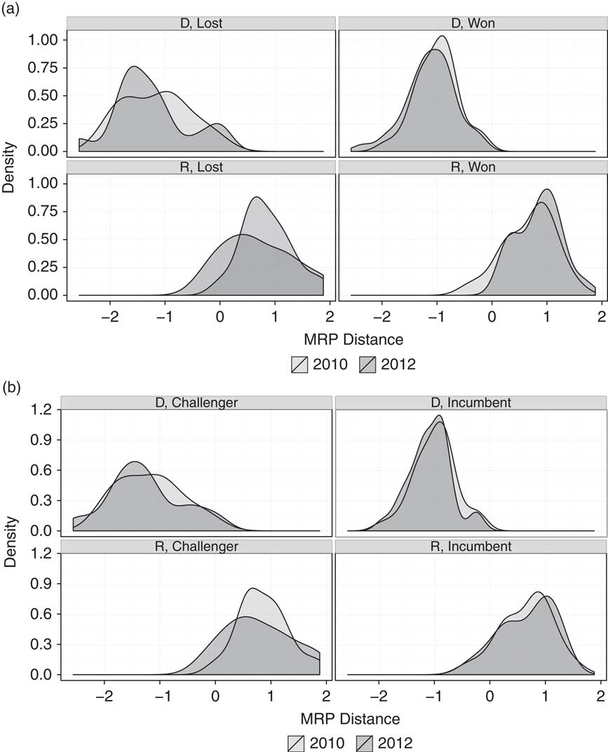
Fig. 4 Spatial distances between voters and candidates by candidate type and year (a) The distance between district means and candidate positions (b) Elected officials before and after reform
There is thus no evidence here that California’s electoral reforms have improved representation, at least in the first post-reform election. In part, this could be a “carry over” effect, because many incumbents elected under the past rules have static ideological positions. If this is the case, we should see a set of “out of touch” incumbents, but we ought to observe a much closer fit between candidates and voters among challengers, especially in 2012, given the creation of more competitive districts. In fact, as Figure 4(b) shows, incumbents are on average closer to average voters than challengers are.Footnote 10 This is, after all, how they became incumbents in the first place. Groseclose (Reference Groseclose2001) provides an intuition about why this might be so. His theoretical model suggests candidates attempt to minimize spatial distances relative to challengers so as to win elections using their valence advantages, like name recognition. Yet, it is discouraging for reformers hoping that, as today’s incumbents eventually leave office, they will necessarily be replaced by challengers located closer to each district’s average voter.
Why did the reforms not bring an immediate improvement in representation? Tests of our more specific hypothesis suggest that voters in California, when they are not guided by party labels, are unable to vote according to the spatial model in the way that the theories behind reform dictate. First, we examine the expectation of Hypothesis 2 that, when two candidates of the same party advance from the top-two primary, November voters will be able to distinguish between the positions of these co-partisans to elect the candidate closest to the district’s average voter. There were seven congressional districts that featured these sorts of same-party runoffs. In three of them, the candidate closest to the district’s mean voter won (Paul Cook in CD8, Eric Swalwell in CD15, and Gloria Negrete McCleod in CD35). Yet, in three other districts, the candidate located further away from the average voter won (conservative Republican Gary Miller in the Democratic-leaning CD31, Lucille Royball-Allard in CD40, and Janice Hahn in CD 44). The two contestants in CD30, Brad Sherman and Howard Berman, were essentially identical in their policy positions. In sum, the candidate closer to a district’s ideological center won in only half of these same-party runoffs, explaining why one hope of the top-two reform went unfulfilled and overall representation did not improve.
Finally, contrary to the expectation in Hypothesis 3 that more competitive districts will yield a better fit between lawmakers and voters, we find no such link. The correlation between district competitiveness (measured by the percentage point difference in major party registration) and squared distance to the district median is a mere 0.09. Perhaps, because candidates running in California’s few competitive districts face pressures to conform to party and interest group discipline in order to raise the money necessary for close campaigns, they are not able to converge on the district median in a Downsian manner. An independent redistricting process did indeed deliver a handful more swing congressional districts, but these did not produce better representation.
Discussion
Our analysis provides a clear lesson for the immediate impact of California’s twin electoral reforms of 2012: neither the Citizens Redistricting Commission nor the top-two primary immediately halted the continuing partisan polarization of California’s elected lawmakers or their drift away from the average voter in each district. This may change in the future, and the voting behavior of those elected in 2012 may become different from the policy positions that they took in their campaigns, with recent work by Grose (Reference Grose2014) and by McGhee (Reference McGhee2015) yielding different verdicts on the impact of California’s reform. More elections and legislative session will provide more information, but for now our results points to the conclusion that these reforms did not fulfill their promise of fundamentally reshaping California politics by electing legislators who were better ideological fit with their districts.
More broadly, this project identifies a new way to study political representation, a concept that is manifestly important on normative grounds. We introduce a relatively low-cost method of studying representation in many districts over time, demonstrating both its empirical validity and its substantive utility. We have used it to see which types of elections lead to better representation, but this measure of ideological congruence could also be used to see which types of district or which types of lawmakers provide better representation of voters in a variety of federal and state contexts. Scholars could also implement this method in other nations or subnational units, as long as they can gather sincere position taking by lawmakers, a representative sample of voters asking them to take a position on these issues, and data on district characteristics that are predictive of voter positions.
Studies of representation are dramatically improving in today’s data revolution. Our method has a niche in this field. Previous attempts like Bafumi and Herron (Reference Bafumi and Herron2010) put voters and lawmakers on the same ideological scale, but need enormous sample sizes in order to get the district-based estimates of representation that make hypothesis testing possible. This approach might be beyond the funding scope of most researchers. Butler and Nickerson (Reference Butler and Nickerson2011) leverage an innovative field experiment to ask whether learning about district preferences pushes legislators into line with voters, but polling on bills that may be amended throughout the legislative process introduces logistical complexity to this approach. Tausanovitch and Warshaw (Reference Tausanovitch and Warshaw2013) pool responses across many polls and use MRP to obtain district-based estimates of opinion that will stimulate much research, but do not put voters and lawmakers on the same scale.
We present a method of measuring the ideologies of voters, legislators, and losing candidates together on a single scale and doing so across districts and years for the price of a single survey with 1000 respondents. Other scholars could conduct a similar survey and use this approach in any political system in which candidates take clear issues positions and district-level demographic data on voters is available. Future research could also go beyond what we have done by estimating the average positions for members of different parties, different ethnic groups, or members of different income quartiles in order to see what type of voter is best represented in a legislature. Such extensions could open up new ways to address, either over time or across different types of districts, the factors that improve congruence between politicians and a range of constituencies. While our study does not have that scope, it provides a replicable way for political scientists to ask a substantively important question that resonates with scholars and reformers alike: What leads to better legislative representation?


