


Introduction
For decades, U.S. research and policy targeted farm retention (Ahearn, Yee, and Korb Reference Ahearn, Yee and Korb2005; Akobundu et al. Reference Akobundu, Alwang, Essel, Norton and Tegene2004; Goetz and Davlasheridze Reference Goetz and Davlasheridze2017). However, an increasingly large proportion of the U.S. food and fiber supply chain is off-farm and encompasses economic activity such as producer services, manufacturing, transportation, warehousing, wholesaling, and retail trade, extending beyond traditional agricultural industrial classifications. The agricultural supply chain is an important component of rural economies, resulting from rural and often region-specific production of agricultural commodities. Productivity and locational changes in off-farm food and agricultural industry (FAI) sectors will influence on-farm activity, and the resulting effects, upstream and downstream from the farm, can have important feedback effects on agricultural producers. Despite their importance, the attributes associated with FAI locations along the agricultural supply chain, such as agricultural support services and farm-related manufacturers and wholesalers, have not been thoroughly explored.
A key barrier to modeling FAI industry locational outcomes has been the availability of comprehensive and accurate data, particularly for smaller rural economies. The relatively limited county-level counts of agriculture-related businesses in rural areas lead to heavy suppression of publicly available data on these establishments, resulting in either incomplete, inaccurate, or biased data and data estimates (Carpenter, Van Sandt, and Loveridge Reference Carpenter, Van Sandt and Loveridge2022c). Since agricultural support services are often geographically bound by the type of crop they support, the heavily censored publicly available data sets that are available contain many zeros, further complicating the process of modeling their locational outcomes. Researchers have hitherto been constrained to use either highly aggregated data or estimated point data of unknown error.
The objective of this article is to demonstrate the potential value of modeling FAI establishment locations using restricted access microdata on multiple industry size measures in the Federal Statistical Research Data Center (FSRDC) system.Footnote 1 To achieve this objective, we use FSRDC restricted access data to first econometrically estimate the determinants of FAI locational outcomes for Support Activities for Agriculture and Forestry (North American Industrial Classification System [NAICS] 115), a relatively aggregated industry that is commonly used in response to public data suppressions (Hertz and Zahniser Reference Hertz and Zahniser2013).Footnote 2 Then, we examine its subsectors – Support Activities for Crop Production (NAICS 1151), Support Activities for Animal Production (NAICS 1152), Support Activities for Forestry (NAICS 1153) – using the same approach. The FSRDC data make several improvements over public or proprietary data, which have limitations that are especially constraining in locational outcome research.Footnote 3 Much of the literature revolving around business locational outcomes measures industry size by the number of establishments within an industry and region (Carpenter, Van Sandt, and Loveridge Reference Carpenter, Van Sandt and Loveridge2021).
Several studies explored these measures in other industries at higher levels of industry aggregation, but the confidential nature of this data has restricted its use (Cleary et al. Reference Cleary, Bonanno, Chenarides and Goetz2018). Data aggregations and suppressions not only limit the understanding of industries germane to the agricultural supply chain but also constrain agricultural support efforts and rural economic development. As shown in the results, aggregation across related sectors can mask (and even reverse the direction of) important statistical relationships. In an effort to overcome these issues, researchers often resort to proprietary data sets with unpublished suppressed cell estimation techniques, or to estimating suppressed cells with their own algorithms. Both solutions yield biased estimates (Carpenter, Van Sandt, and Loveridge Reference Carpenter, Van Sandt and Loveridge2022c).
The Longitudinal Business Database (LBD) is an annual series produced by the U.S. Census Bureau based on establishment records from the Business Register (Jarmin and Miranda Reference Jarmin and Miranda2002). The LBD remains a core data set for studying the characteristics and determinants of entry, growth, and exit at the establishment, firm, industry, and economy-wide level (Carpenter and Loveridge Reference Carpenter and Loveridge2018, Reference Carpenter and Loveridge2019, Reference Carpenter and Loveridge2020; Davis, Faberman, and Haltiwanger Reference Davis, Faberman and Haltiwanger2006; Foster, Haltiwanger, and Krizan Reference Foster, Haltiwanger and Krizan2006; Haltiwanger, Jarmin, and Miranda Reference Haltiwanger, Jarmin and Miranda2013). The Integrated Longitudinal Business Database (ILBD) covers non-employers.Footnote 4 Longitudinal establishment-level data that encompass an entire state or regional economy are similarly becoming available in other countries, with economists often using them to examine firm establishment locations, though FAI locational analysis remains relatively neglected (Arauzo-Carod and Viladecans-Marsal Reference Arauzo-Carod and Viladecans-Marsal2009; Chen and Moore Reference Chen and Moore2010; Devereux, Griffith, and Simpson Reference Devereux, Griffith and Simpson2007; Figueiredo, Guimaraes, and Woodward Reference Figueiredo, Guimarães and Woodward2002; Holl Reference Holl2004).
An FSRDC is thus a natural place to make improvements to research. Researchers cannot release minimum or total counts, but we develop unbiased coefficients in regression results. By using the LBD, ILBD, and publicly available county-level data, we propose improving existing FAI location research by:
-
1. Increasing accuracy in industry size measurement by comparing location determinants of both employer establishments and non-employer establishments.
-
2. Reducing generalizability by expanding geographic scope.
-
3. Testing the influence of industry aggregation on FAI location outcome models.
The next section summarizes prior research on FAI locational outcomes. Then, we review related econometric and data issues. This review leads to our flexible approach in the supporting example empirical method, which uses FSRDC data. The example results section demonstrates that significant location attributes of FAI vary depending on the type and level of industry in the FAI supply chain. We note different data generation processes not only across different FAI but also between employers and non-employers within a specific industry.Footnote 5 In most FAI, agricultural production variables are important contributors to the likelihood of a county containing at least some FAI establishments, as well as the number of establishments. We also show that aggregating sectors can lead to substantial changes in the magnitude, significance, and even direction of estimated coefficients. The article concludes by summarizing our review and supporting modeling exercise to achieve our objective of demonstrating the value of FSRDC data and flexible modeling in accurately modeling FAI locational outcomes.
FAI locational research
Using FSRDC microdata, Dunn and Hueth (Reference Dunn and Hueth2017) show the number of crop services establishments is in secular decline, but the number of employees per establishment is growing. The authors also show that multi-unit establishments make up a relatively constant and small proportion of that sector and that business establishment births are in decline. Consolidation to exploit economies of scale in FAI is therefore likely an ongoing process that involves firms deciding to stay in business at their current location, to grow at their current location, go out of business, or move. This observation has two implications for FAI location research:
-
1. The classic location question from industrial recruitment literature, that is, how to attract a branch plant, takes on a slightly different form with FAI, implying a need to explore fully characteristics associated with viability of existing locations rather than focusing exclusively on decisions involving new locations.
-
2. A secular trend towards fewer and larger FAI establishments translates into more counties with suppressed data, leading to a need to aggregate across industries for a full data set. Aggregation can produce important shortcomings in estimations, as critical locational factors for one industry may be very different than another, even if they occupy the same two-digit NAICS sector. Thus, over time, as the number of suppressions grows, models based on public data may become less accurate.
Modeling approaches from industrial recruitment inform our analytical choices in exploring determinants of FAI firm locations. In the context of rural areas (non-FAI), manufacturing arises from several conditions. Importantly, the location choice literature reveals that rural areas can be attractive to manufacturing firms because wages, property taxes, and land costs can be lower than in metro areas, though rural workforce size can be a limitation. Unfortunately, research into rural manufacturing locational outcomes remains hamstrung by rural data suppression, which worsen with industry disaggregation.
A demand threshold is defined as the minimum market size (population) required to support a particular type of retail or service business and still yield a rate of return such that the business will continue to operate (Berry and Garrison Reference Berry and Garrison1958a and Reference Berry and Garrison1958b; Parr and Denike Reference Parr and Denike2016). In examining off-farm FAI service industries, such as agricultural support services, we draw on past retail and service industry demand threshold analysis. Cleary et al. (Reference Cleary, Bonanno, Chenarides and Goetz2018) adapt Bresnahan and Reiss (Reference Bresnahan and Reiss1991) to estimate the minimum market size (population thresholds) that imply profitability for one or more large grocery stores in non-metro U.S. counties. The intuition is straightforward, with lower population thresholds implying store profitability in less populated areas. Their results suggest that the cost-effectiveness of broad-based policy solutions to improve physical access to large food stores or to stimulate demand may be limited. Similarly, threshold analyses could serve as a useful tool to highlight over-investment in off-farm FAI, such as may be the case with food hubs (Cleary et al. Reference Cleary, Goetz, Mcfadden and Ge2019). More specific FAI and FAI-related threshold analyses and more precise policy implications are now possible with the FSRDC system.
For off-farm FAI manufacturing, most research focuses on the locational determinants of food processing and food manufacturing. Typically, these studies only examine a specific geographic region, probably due to non-disclosures. Food manufacturing locations tend to occur in counties with access to input and product markets, developed transportation networks, agglomeration economies (efficiencies that occur when industries locate near each other and industrial clusters), favorable fiscal policies, and low wages (Davis and Schluter Reference Davis and Schluter2005; Henderson and McNamara Reference Henderson and McNamara1997, Reference Henderson and McNamara2000). Particularly, important factors include proximity of agricultural commodities and low-cost labor. Rural counties tend to historically have a comparative disadvantage for attracting food processors, though non-metropolitan counties adjacent to urban areas may have an advantage for some food manufacturers (Lambert and McNamara Reference Lambert and McNamara2009). Studies enhancing the understanding of agglomeration economies may be particularly important for rural areas, where there may be possible negative effects of competition from growing concentrations of firms (Schmit and Hall Reference Schmit and Hall2013). Consolidation under spatial monopsony may also result in unserved areas.
Less discussed in prior location modeling efforts is the role of industry aggregation from nesting more refined industry categories in limiting the accuracy of model outcomes. This may be a function of prior limits on alternative levels of aggregation. In contrast, aggregation bias is familiar to analysts working in international trade (Feenstra and Hanson Reference Feenstra and Hanson2000; Hillberry Reference Hillberry2002) or regional economic models using input-output or CGE approaches (Miller and Blair Reference Miller and Blair2009). Wensley and Stabler (Reference Wensley and Stabler1998) refer to this industry aggregation issue as the product mix effect. They find that their demand threshold models on subsector classifications within the NAICS system that include many more narrowly defined industries more often exhibit increasing establishment multiplication rates. Despite Wensley and Stabler’s (Reference Wensley and Stabler1998) comment on the potential issue of the product mix effect from industry aggregation, most demand threshold studies count establishments at the subsector or industry group levels (Chakraborty Reference Chakraborty2012; Mushinski and Weiler Reference Mushinski and Weiler2002; Reum and Harris Reference Reum and Harris2006; Shonkwiler and Harris Reference Shonkwiler and Harris1996).
Clearly, there are also disadvantages in finer levels of disaggregation. No two businesses are alike; at some point of disaggregation, more output becomes cumbersome, suggesting diminishing marginal returns from disaggregation, particularly in sector classifications with small product mixes. The number of zero values across geography will also grow with greater sectoral detail. Within the FSRDC system, it becomes more feasible to test various levels of aggregation. In the analysis that follows, we explore results associated with two levels of NAICS code aggregation. The next section provides a basis for the model structure used in our analysis.
Estimation methods in the context of FAI
This section first outlines estimation methods of traditional locational choice and demand threshold literatures before weighing the trade-offs with several different estimators, largely following the recent review by Carpenter, Van Sandt, and Loveridge (Reference Carpenter, Van Sandt and Loveridge2021) and applying their guidance to the FAI context.
Carlton (Reference Carlton1983) and Bartik (Reference Bartik1985) are among the first to model the determinants of business location using multinomial logit (McFadden Reference McFadden and Zarembka1973). Limitations of this approach include an excessive number of alternatives and violation of the independence of irrelevant alternatives (IIA) assumption, given the location alternatives are likely correlated, even when conditioning on observable characteristics (Wooldridge Reference Wooldridge2010). Researchers aggregated alternatives to address the excessive alternatives problem and attempted to control for the IIA violation by introducing spatial group indicator variables (Bartik Reference Bartik1985).Footnote 6 Despite these efforts, the limitations led to use of nested logit, which uses a smaller sample of alternatives randomly drawn from the full set of alternatives (Friedman et al. Reference Friedman, Gerlowski and Silberman1992; Woodward Reference Woodward1992). This approach faces limitations both in the imposition of an arbitrarily limited and hierarchical choice set on firms, and the implied reduction in information. Furthermore, both approaches are limited because they are only consistent if the IIA assumption holds within subsets of the alternatives, that is, various hierarchies for the nested logit and spatial groups for the multinomial logit.
Given these limitations, others model establishment location by using count data models to examine locational outcomes in a particular area (Coughlin and Segev Reference Coughlin and Segev2000; Guimarães, Figueiredo, and Woordward Reference Guimarães, Figueiredo and Woodward2004; Papke Reference Papke1991; Wu Reference Wu1999). Importantly, Guimarães, Figueiredo, and Woodward (Reference Guimarães, Figueiredo and Woodward2003, Reference Guimarães, Figueiredo and Woodward2004) demonstrate not only that the Poisson count model presents a more tractable approach than conditional logit approaches but also that the coefficients of the Poisson model can be given an economic interpretation compatible with the framework of random utility (profit) maximization. Conveniently in the context of FAI, which include both services/retail and manufacturing, count data models are also compatible with the Central Place Theory (CPT) theoretical perspective, which researchers use in demand threshold analysis of retail and service sectors (Carpenter, Van Sandt, and Loveridge Reference Carpenter, Van Sandt and Loveridge2021). Furthermore, the count data regression is preferred when dealing with large sets of alternatives, since each spatial alternative becomes an observation, and thus, the excessive choice set problem faced by logit models becomes an advantage (Guimarães, Figueiredo, and Woodward Reference Guimarães, Figueiredo and Woodward2003).
When modeling demand threshold and business location using count data, multiple theoretical dimensions can be considered. First, the location or “participation” decision $\left\{ {0,\;1} \right\}$
and the establishment count or “amount” decision
$\left\{ {0,\;1} \right\}$
and the establishment count or “amount” decision $\left\{ {0,\;1,\;2,\;3,\; \ldots } \right\}$
may be separate for FAI (and understanding each decision may be of interest), so a flexible estimator that models the decisions separately (with a zero-inflated estimator) is preferable. Relatedly, the effect of explanatory variables on the respective participation and amount decisions may have different partial effects, and there may be conditional correlation between the participation distribution and the amount distribution. Finally, both the participation and amount decision allow for the possibility of zero values. For establishment location data, there may be two types of zeros: (1) structural zeros – locations that establishments will never choose for participation; and (2) non-structural zeros – locations that establishments could potentially choose but are not chosen.
$\left\{ {0,\;1,\;2,\;3,\; \ldots } \right\}$
may be separate for FAI (and understanding each decision may be of interest), so a flexible estimator that models the decisions separately (with a zero-inflated estimator) is preferable. Relatedly, the effect of explanatory variables on the respective participation and amount decisions may have different partial effects, and there may be conditional correlation between the participation distribution and the amount distribution. Finally, both the participation and amount decision allow for the possibility of zero values. For establishment location data, there may be two types of zeros: (1) structural zeros – locations that establishments will never choose for participation; and (2) non-structural zeros – locations that establishments could potentially choose but are not chosen.
Review of corner response and count data models
Given the nature of the establishment data, $y \in \left\{ {0,\;1,\;2,\;3,\; \ldots } \right\}$
, count data models are most appropriate for empirical estimation.Footnote
7
Indeed, count data estimators have become common in locational and threshold models, though researchers often fail to appropriately apply and compare the various models, as we will demonstrate. For non-FAI establishments, applications of Poisson, Negative Binomial (NB), Hurdle Poisson (HP), and Zero-Inflated Poisson (ZIP) are numerous with Carpenter, Van Sandt, and Loveridge (Reference Carpenter, Van Sandt and Loveridge2021) providing a near comprehensive review for each. They also show a place for the Zero-Inflated Negative Binomial (ZINB), especially when using an expanded geographic scope.
$y \in \left\{ {0,\;1,\;2,\;3,\; \ldots } \right\}$
, count data models are most appropriate for empirical estimation.Footnote
7
Indeed, count data estimators have become common in locational and threshold models, though researchers often fail to appropriately apply and compare the various models, as we will demonstrate. For non-FAI establishments, applications of Poisson, Negative Binomial (NB), Hurdle Poisson (HP), and Zero-Inflated Poisson (ZIP) are numerous with Carpenter, Van Sandt, and Loveridge (Reference Carpenter, Van Sandt and Loveridge2021) providing a near comprehensive review for each. They also show a place for the Zero-Inflated Negative Binomial (ZINB), especially when using an expanded geographic scope.
The Poisson model remains useful at least as a starting point for comparison to other estimation procedures. However, the Poisson model’s assumption that the conditional variance of the dependent variable is equal to the conditional mean is often violated in practice due to multiple potential sources of overdispersion. If the conditional distribution is overdispersed, the NB will be more efficient than Poisson. The NB allows for unobserved heterogeneity between subjects that implies overdispersion. Specifically, the NB assumes the Poisson parameter is Gamma distributed and allows the amount of overdispersion to increase with ${\rm{E}}\left( {{y_i}|{x_i}} \right)$
(Wooldridge Reference Wooldridge2010).
Footnote 8
Although this likely holds when modeling FAI employment (e.g., due to rare large FAI manufacturers), this relationship is unlikely to hold when measuring FAI establishments due to excess zeros driving much of the overdispersion while decreasing
${\rm{E}}\left( {{y_i}|{x_i}} \right)$
(Wooldridge Reference Wooldridge2010).
Footnote 8
Although this likely holds when modeling FAI employment (e.g., due to rare large FAI manufacturers), this relationship is unlikely to hold when measuring FAI establishments due to excess zeros driving much of the overdispersion while decreasing ${\rm{E}}\left( {{y_i}|{x_i}} \right)$
. Hence, zero-inflated and hurdle versions of the Poisson model are often used to account for excess zeros in the data. Zero-inflated models add a logit link function which allows for an inflation stage in which the probability of an outcome being a structural zero is estimated, while still allowing for the estimation of (non-structural) zeros in the typical Poisson.Footnote
9
This results in two sets of estimates: (1) coefficients describing the likelihood of an observation being a structural zero and (2) coefficients describing changes in the level of the dependent variable given the observation is not a structural zero. Conversely, HP only assumes one type of zero by truncating the Poisson distribution after the zero-generating process. Such a restriction would be difficult to justify for any off-farm FAI under consideration here, so we do not test the HP. See Carpenter, Van Sandt, and Loverdige (Reference Carpenter, Van Sandt and Loveridge2021) for more details.
${\rm{E}}\left( {{y_i}|{x_i}} \right)$
. Hence, zero-inflated and hurdle versions of the Poisson model are often used to account for excess zeros in the data. Zero-inflated models add a logit link function which allows for an inflation stage in which the probability of an outcome being a structural zero is estimated, while still allowing for the estimation of (non-structural) zeros in the typical Poisson.Footnote
9
This results in two sets of estimates: (1) coefficients describing the likelihood of an observation being a structural zero and (2) coefficients describing changes in the level of the dependent variable given the observation is not a structural zero. Conversely, HP only assumes one type of zero by truncating the Poisson distribution after the zero-generating process. Such a restriction would be difficult to justify for any off-farm FAI under consideration here, so we do not test the HP. See Carpenter, Van Sandt, and Loverdige (Reference Carpenter, Van Sandt and Loveridge2021) for more details.
Finally, previous research failed to account for overdispersion that remains after the zero inflation in ZIP (Carpenter, Van Sandt, and Loveridge Reference Carpenter, Van Sandt and Loveridge2021). This remaining overdispersion may result from unobserved heterogeneity between subjects and excessive concentration of firms, which itself increases in economies of scale and agglomeration. Such economies are common to off-farm FAI. Thus, ZINB is underutilized in the current literature, with examinations of FAI typically using NB due to overdispersion, but failing to test for the source of that overdispersion (Bhattacharya and Innes Reference Bhattacharya and Innes2016; Henderson and McNamara Reference Henderson and McNamara2000; Lambert and McNamara Reference Lambert and McNamara2009; Weiss and Wittkopp Reference Weiss and Wittkopp2005). Indeed, we highlight that ZINB is the preferred model for numerous off-farm FAI.
Review of off-farm FAI data sources and issues
As noted above, researchers typically measure industry size in a location with establishment counts. Despite the growing body of literature highlighting effective econometric methods to measure demand thresholds on establishment counts in rural areas, extant demand thresholds research focuses on retail businesses almost exclusively and is limited in detail, or limited in industrial and geographic scope due to data limitations (Chakraborty Reference Chakraborty2012). Indeed, many demand threshold analysis and locational analysis studies use the publicly available County Business Patterns (CBP) data, resulting in several limitationsFootnote 10 and biased estimates (Carpenter, Van Sandt, and Loveridge Reference Carpenter, Van Sandt and Loveridge2022c).
Other federal data programs publish information about the economic activity in FAI, including the National Establishment Time-Series (NETS), Quarterly Census of Employment and Wages (QCEW), the Quarterly Workforce Indicators (QWI), and Non-employer Statistics (NS).Footnote 11 Although versions of the QCEW, QWI, and NS are available publicly, researchers encounter the same problem as the CBP data: the exact counts of a particular NAICS code are often suppressed. While the NETS data avoid issues with suppressions and include non-employers, it remains a smaller sample (while the LBD is essentially the universe of establishments in its frame), and thus, researchers often must pool NETS observations across multiple years to reach sufficient observations of FAI (Low et al. Reference Low, Bass, Thilmany and Castillo2020). Isserman and Westervelt (Reference Isserman and Westervelt2006) provide methods to improve over simply taking the midpoint from suppressed CBP data and numerous proprietary data sets exist that estimate suppressed cells. However, these data sets remain substantially biased, with estimates ranging from 30% attenuation bias in 3-digit NAICS county-level data to being unreliable in 5- and 6-digit NAICS data (Carpenter, Van Sandt, and Loveridge Reference Carpenter, Van Sandt and Loveridge2022c). Suppressions are particularly prevalent in some FAI due to their relatively small count in rural counties. Given the extensiveness of disclosure limitations, exact counts yield more precise models. Finally, the LBD includes all off-farm FAI establishments with paid employees without regard to whether any employees are engaged in agricultural production. An FSRDC is thus a natural place to make improvements to existing research.
Example empirical approach
In support of the objective of this paper – to demonstrate the potential value of federal administrative data for food and agricultural industry (FAI) locational outcome research – we conduct an example empirical approach. First, we compare results and model diagnostics from the Poisson, NB, and their zero-inflated counterparts to provide robust results across NAICS 115, 1151, 1152, and 1153. This flexible approach takes advantage of the count nature of the data and allows for the separate analysis of factors contributing to both structural zeros and non-structural, while also addressing the multiple potential sources of overdispersion. We selected the data generation process underlying each industry by first testing for overdispersion in the data to select between the Poisson and negative binomial distributions. After checking for zero inflation, the alpha parameter was double-checked to ensure that overdispersion was still present in the data after accounting for excess zeros.
The log-likelihood function for ZIP may be written as:
 \begin{align}\ln L &= \mathop \sum \limits_{i \in {\rm{S}}} {\rm{ln}}\left\{ {{\rm{F}}\left( {\gamma '{Z_i}} \right) + \left[ {1 - {\rm{F}}\left( {\gamma '{Z_i}} \right)} \right]\ {\rm{exp}}\left( { - {\lambda _i}} \right)} \right\}\\
&\quad + \mathop \sum \limits_{i \notin {\rm{S}}} \left\{ {\ln \left[ {1 - {\rm{F}}\left( {\gamma '{Z_i}} \right)} \right] - {\lambda _i} + {y_i}\beta '{X_i} - \ln \left( {{y_i}!} \right)} \right\}\end{align}
\begin{align}\ln L &= \mathop \sum \limits_{i \in {\rm{S}}} {\rm{ln}}\left\{ {{\rm{F}}\left( {\gamma '{Z_i}} \right) + \left[ {1 - {\rm{F}}\left( {\gamma '{Z_i}} \right)} \right]\ {\rm{exp}}\left( { - {\lambda _i}} \right)} \right\}\\
&\quad + \mathop \sum \limits_{i \notin {\rm{S}}} \left\{ {\ln \left[ {1 - {\rm{F}}\left( {\gamma '{Z_i}} \right)} \right] - {\lambda _i} + {y_i}\beta '{X_i} - \ln \left( {{y_i}!} \right)} \right\}\end{align}
where S is a set of observations where ${y_i} = 0$
,
${y_i} = 0$
, ${\rm{F}}$
is the logit link function (for zero inflation),
${\rm{F}}$
is the logit link function (for zero inflation), $Z$
is a vector containing covariates in the participation decision, and
$Z$
is a vector containing covariates in the participation decision, and $X$
is a vector containing covariates in the amount decision. The log-likelihood function for ZINB differs from this by allowing the Poisson parameter to be Gamma distributed thereby relaxing the assumption of equidispersion.
$X$
is a vector containing covariates in the amount decision. The log-likelihood function for ZINB differs from this by allowing the Poisson parameter to be Gamma distributed thereby relaxing the assumption of equidispersion.
To choose among the various count data models empirically, much previous work has incorrectly used Vuong’s Statistic to test for zero inflation (Wilson Reference Wilson2015).Footnote 12 To provide a consistent comparison to evaluate the various count data models, we focus on graphical distribution analysis and comparison of the Akaike and Bayesian information criteria (AIC and BIC, respectively) as suggested in Greene (Reference Greene1994). If an industry follows a zero-inflated data generation process, we retest the overdispersion parameter again to ensure the overdispersion was not solely a product of the zero-inflation process.
Off-Farm FAI data
We use restricted access establishment-level data from the Census’ LBD and ILBD for the year 2014, along with secondary data sources to econometrically estimate the locational outcomes for the more-aggregated Support Activities for Agriculture and Forestry (NAICS 115), along with its (less-aggregated) sub-industries Support Activities for Crop Production (NAICS 1151), Support Activities for Animal Production (NAICS 1152), and Support Activities for Forestry (NAICS 1153). Table 1 provides summary statistics for these industries.
Food and agricultural industry summary statistics

Note: Due to disclosure concerns, these statistics come from publicly available census county business patterns and non-employer statistics data.
Despite the inclusion of all businesses within the LBD and the ILBD, the U.S. Census Bureau requires us to conduct our analysis at an aggregated county level due to the sensitivity of the data. This unit of analysis is also necessary for including important secondary data sources that capture the potential influence of internet access, travel infrastructure, labor characteristics, urban influence, and other demographic and location variables. Further, county-level aggregation facilitates the implementation of the previously discussed methods. Table 2 provides descriptive statistics for the publicly available county-level FAI data and sources. A subset of FAI is selected to demonstrate the empirical implications of industry aggregation and size measurement in the results section.
Covariate descriptive statistics and sources
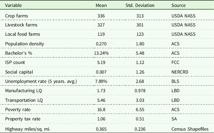
Note: Table provides some descriptive statistics for model covariates and their respective sources. Local food farms are defined by USDA NASS (direct to consumer/retailer, agritourism, and value-added products). Descriptive statistics for the LQ are reproduced using publicly available U.S. Census County Business Pattern to assuage disclosure concerns.
Abbreviations: ACS: American Community Survey; BLS: Bureau of Labor Statistics; FCC: Federal Communications Commission; LQ: Locational Quotient; NASS: National Agricultural Statistics Service; NERCRD: Northeast Regional Center for Rural Development at Pennsylvania State University; SA: SmartAsset.com; USDA: United States Department of Agriculture.
This article does not estimate the locational outcomes of farms and ranches, but rather agricultural support services (i.e., 115, 1151, 1152, and 1153). As we describe in the next section, results vary by industry and sub-industry.
While FAI includes dozens of industry types spanning many sectors of the economy, we focus on investigating this subset of these industries with a 2014 cross section of the data using every county in the continental U.S. With the intention of highlighting the multitude of potential directions of FAI location outcomes research in the FSRDC system, we provide a diverse and large set of covariates routinely found in the location determinants literature (Carpenter, Dudensing, and Van Sandt Reference Carpenter, Dudensing and Van Sandt2022a; Carpenter et al. Reference Carpenter, Van Sandt, Dudensing and Loveridge2022b; Henderson, Kelly, and Taylor Reference Henderson, Kelly and Taylor2000; Lambert and McNamara Reference Lambert and McNamara2009; Van Sandt et al. Reference Van Sandt, Carpenter, Dudensing and Loveridge2021a; Reference Van Sandt, Carpenter, Dudensing and Loveridge2021b) and to facilitate comparisons across different measures of industry size (e.g., non-employer establishments and employer establishments), covariates are the same across industries. More specifically, each model uses 2014 county-level data and includes production variables (crop farm counts, livestock farm counts, and share local food farms), place-based factors (population density and internet service providers), labor-force characteristics (social capital index, share with a bachelor’s degree or higher, share in poverty, and the unemployment rate), industrial sector interdependencies (manufacturing location quotient, and transportation and wholesale location quotient), and factor costs (property tax rate and highway density).Footnote 13
Example results
Tables 3 and 4 summarize the information criteria tests across support services and sub-industries for both employer establishments and non-employer establishments, respectively. The resulting distribution is itself indicative of economic and administrative features. For example, the NB distribution amongst employer establishments in Support Activities for Forestry (NAICS 1153) indicates these establishments can operate in most locations and likely serve smaller, more rural communities where market demand is not great enough to support larger employers more common in Support Activities for Crop Production (NAICS 1151) and Support Activities for Animal Production (NAICS 1152).Footnote 14 Hence, industry aggregation also influences researchers’ ability to identify the data generation process, with the more-aggregated Support Activities for Agriculture and Forestry (NAICS 115) preferring ZINB and obscuring this nuance. Thus, research questions specific to an industry subset of an aggregated NAICS suffer not only from estimated coefficients values being confounded by other industries’ noise but also from the inability to select the industry’s correct data generation process.
Information criteria for employer establishments
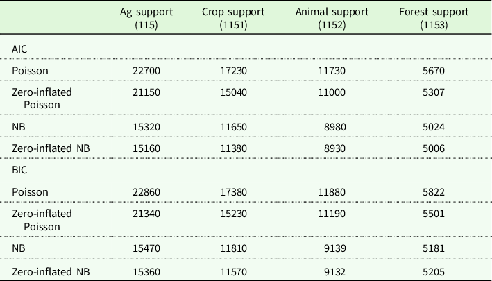
Note: Table shows the Akaike and Bayesian information criteria (AIC and BIC, respectively) across count data estimators for employer establishments in 2014. NB is negative binomial.
Information criteria for non-employer establishments
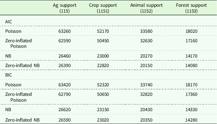
Note: Table shows the Akaike and Bayesian information criteria (AIC and BIC, respectively) across count data estimators for non-employer establishments in 2014. NB is negative binomial.
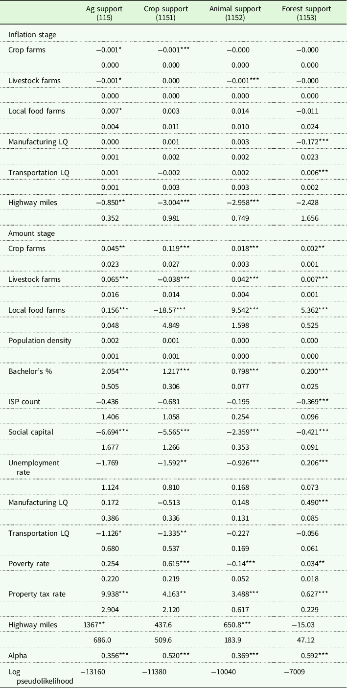
The marginal effects for our example industries are presented in Tables 5 and 6 to demonstrate the effect on model coefficients from (1) different levels of industry aggregation, which we discuss based on the difference between results for NAICS 115 compared to 1151, 1152, and 1153; and (2) different measures of industry size, which we discuss based on the difference between results for employers and non-employers. Of course, there exist unobservable variables that may affect location and correlate with explanatory variables, so we again emphasize the associative and non-causal interpretation of these example results, while focusing on (1) and (2).
Employer establishment locational determinants results
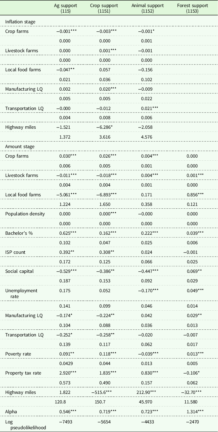
Note: Table shows the results across Ag support services and its subsectors when using county-level employer establishment counts as unit of analysis. Forest support (NAICS 1153) shows no inflation stage because the information criteria testing preferred negative binomial to zero-inflated negative binomial (see Table 5).
Abbreviations: Bachelors %, percent of the population with a bachelor’s degree or higher; ISP, internet service provider; LQ, location quotient.
Significance levels: ***p < 1%, **p < 5%, *p < 10%.
Non-employer establishment locational determinants results
Note: Table shows the results across Ag support services and its subsectors when using county-level non-employer establishment counts as unit of analysis.
Abbreviations: Bachelors %, percent of the population with a bachelor’s degree or higher; ISP, internet service provider; LQ, location quotient.
Significance levels: ***p < 1%, **p < 5%, *p < 10%.
In all zero-inflated models, the logistic function predicts whether a county is a structural zero. Thus, the negative coefficients in the inflation stage of Tables 5 and 6 indicate that an increase in the variable is expected to lead to a decrease in the likelihood of the county being a structural zero. Following a priori expectations, the presence of agricultural production businesses corresponds to a smaller likelihood of a county being a structural zero for 115, 1151, and 1152 for both employer and non-employer establishments. Inflation stage results also show a positive association between above-average manufacturing industry concentration and a county having zero crop support services (1151) structurally, and a positive association between transportation industry concentration and a county having animal support services (1152) structurally. Researchers examining the more-aggregated agricultural support services (115) would find statistically insignificant coefficients for both manufacturing and transportation location quotients.
To examine the effects of different levels of industry aggregation, in the agricultural and forestry support services industries, we compare the marginal effects in the amount stage presented in Tables 5 and 6 across the more-aggregated NAICS 115 with its three subsectors. Results suggest that aggregating industries can influence the magnitude, direction, and statistical significance of locational factors for establishments involved in support activities for crop and animal production. This finding is clear when examining the association of crop farms and livestock farms with the location of support services establishments. For example, Table 5 shows that local livestock producers have a negative relationship with the more-aggregated Support Activities for Agriculture and Forestry (NAICS 115), but that this is driven by the relationship with Support Activities for Crop Production (1151), while the relationship with Animal Support Services (1152) and Forestry Support Services (1153) reverses direction and is positive. The relationship between crop farms and our selection of industries is positive, but varies in statistical significance and is statistically insignificant for Forestry Support Services. This statistically significant variation and sign reversal occurs across a number of variables common to location choice research, including the share of the population with a bachelor’s degree, social capital, unemployment rate, industrial location quotients, poverty rate, property tax rate, and highway miles. To summarize, using industry classifications that are more broadly defined than implied by a research question leads to statistically significant over- or underestimating the influence of important location factors specific to a sub-industry of interest.
To examine the effect of using different measures of industry size, we compare marginal effects estimated with employer establishments (Table 5) to marginal effects with non-employer establishments (Table 6). The differences between these associations are statistically significant for multiple covariates. For example, livestock farms have a negative association with the number of employer businesses in the aggregated 115, but a large positive association with the number of 115 non-employer businesses. (The sub-industries are more stable directionally.) The association between the local poverty rate and the aggregated 115 loses statistical significance for non-employers, while the sub-industries maintain significance and directional consistency with employer establishments. More generally, the less-aggregated industries show a much higher share of significant covariates in the amount stage of the models, indicating that more specific industry codes may benefit from less noise resulting from the mix of competing industry-specific nuances in aggregated 115 classifications. In summary, it is clear from the amount stage results that non-employer FAI establishments are different from the locational determinants than employer FAI.
Summary and concluding remarks
An increasingly large share of the food and fiber supply chain has moved beyond the farm gate, leading to FAI being located across different sectors of the economy. Despite this shift, research aimed at selecting factors associated with locational outcomes of these FAI remains difficult, due to the rural nature of FAI and the associated suppression of FAI metrics in publicly available data sets. Previous demand threshold literature circumnavigates this issue by limiting the geographic scope of their study area, aggregating industries to more general classifications, and by adopting econometric methods that may fit and describe the sample but not the population of interest.
Our review and supporting example results using FSRDC data demonstrate the potential value of using FSRDC data to conduct FAI locational analysis at various levels of aggregation. In particular, we show that the choice of industrial aggregation and size measurement often affect the magnitude, sign, and significance of several variables common to locational choice research. Hence, researchers using aggregated FAI industries should take care when generalizing their results (to all sub-industries). Our supporting results make contributions to the literature by employing zero-inflation count data models to restricted access data sets through the Federal Statistical Research Data Center system to estimate demand threshold models for several FAI. We find that while the ZINB data generation process is almost always preferred across FAI. The distributions of these industries reveal important findings: (1) the significant overdispersion present in all FAI signifies the tendency of FAI to cluster; and (2) the variety of agricultural support services have different data generation processes with nuanced structural and sampling zeros.
Estimated coefficients across employers and non-employers show the benefits of more finely disaggregated industry classifications. Notably, in agricultural support services, broader industry classifications lead to underestimation or even sign reversal of statistically significant location factors. The importance of non-employer establishments to rural economies and their different locational determinants compared to employer establishments is also evident through differences in the models’ assumed distributions, the magnitudes of coefficient marginal effects, and the differences in significant coefficients.
Some data limitations persist, even in an FSRDC. For example, researchers cannot comingle USDA NASS (National Agricultural Statistics Service) Census of Agriculture microdata in the FSRDC. Thus, integration of the two data sources requires either taking (suppressed and aggregated) public versions of FSRDC data into the USDA NASS laboratories or taking (suppressed and aggregated) public versions of the NASS data into an FSRDC laboratory. Although the methods section highlights the benefits of using aggregated count data in the context of FAI locational outcomes, future research opportunities would further expand, given the ability to comingle USDA NASS and FSRDC microdata. This comingled data would not only facilitate substantial research on the interplay between on- and off-farm business dynamics over time and with respect to policy (and structural) changes but also improve the seasonal measures of industry size in FAI.
The USDA remains an outlier in their provision of microdata to FSRDC researchers, as current federal entities that allow comingling of data in the FSRDC system (directly or indirectly) include the U.S. Census Bureau, Internal Revenue Service, Bureau of Labor Statistics, Bureau of Justice Statistics, Environmental Protection Agency, National Center for Health Statistics, and Agency for Healthcare Research and Quality, among several others. This policy by USDA is needlessly limiting the research questions researchers can answer with USDA data. Our example results highlight that compelling researchers to use relatively aggregated industry classifications can lead to entirely incorrect conclusions when attempting to generalize to FAI subsectors.
Despite the contributions made here, there are still many research questions that cannot be answered with current public data resources. These questions are not only central to agricultural marketing and economic development, but the livelihoods of the people who depend on FAI as well as other frequently censored industries primarily found in rural areas. With this in mind, we highlight three areas using FSRDC data resources for future research. First, while specific industrial quality comparisons between public and restricted access data are understandably prohibited within the FSRDC, comparisons between restricted access and purchased estimates may reveal the true value of these expensive yet proprietary data sets beyond the broad implications of Carpenter, Van Sandt, and Loveridge (2022).Footnote 15 Second, aggregation bias may vary across space. Western counties are larger than eastern counties, and this may lead to less suppression and aggregation bias. Third, modeling more disaggregated industries within FAI would improve our knowledge of agricultural supply chain location decisions and their impact on rural economies. Finally, the different industry size measures used here could be expanded beyond FAI to explore the data generation and decision processes of other industries and sub-industries, particularly those that may be germane to rural economic development that are often suppressed in public data.
Data availability statement
The data that support the findings for this article are available through the Federal Statistical Research Data Center (FSRDC). For details on how to access the FSRDC system, visit https://www.census.gov/about/adrm/fsrdc.html. Other data are publicly available, with details on sources available in Table 2.
Acknowledgements
The authors thank Rebekka Dudensing and numerous conference participants for their comments on an earlier version of this work. Any opinions and conclusions expressed herein are those of the author and do not necessarily represent the views of the U.S. Census Bureau. All results have been reviewed to ensure that no confidential information is disclosed.
Author contributions
CC, AV, and SL conceived and designed the study. AV conducted data gathering. CC and AV performed statistical analyses. CC, AV, and SL wrote the article.
Funding statement
The project was supported by the Agricultural and Food Research Initiative Competitive Program of the USDA National Institute of Food and Agriculture (NIFA), award numbers 2017-67023-26242 and 2018-68006-27641.
Competing interests
The authors declare none.


 Open access