


Introduction
Atom probe tomography (APT) is an analytical microscopy technique with up to single atom sensitivity in all three dimensions. A needle-shaped specimen with an apex radius of ~50–150 nm is subjected to a high DC voltage. By controlled voltage or laser pulsing, individual atoms are field desorbed from the surface and accelerated toward a position-sensitive detector, where the time of flight and the impact position are recorded (Cerezo et al., Reference Cerezo, Godfrey and Smith1988; Blavette et al., Reference Blavette, Bostel, Sarrau, Deconihout and Menand1993). After the measurement, the evaporated volume of the tip is reconstructed from the detected events to reveal the structural arrangement of the atoms inside the material. Since the exact ion trajectories are not known from the experiment, this reconstruction of the emitter is only possible by assumptions of the emitter's surface during field evaporation.
In most experimental works, the reconstruction follows a simple point projection model assuming a hemispherical apex (Bas et al., Reference Bas, Bostel, Deconihout and Blavette1995). However, in the case of multiphase materials with varying evaporation threshold, the real tip shape changes during the measurement and the projection on a spherical emitter leads to significant distortions in the reconstruction known as local magnification artifacts (Miller & Hetherington, Reference Miller and Hetherington1991; Miller et al., Reference Miller, Cerezo, Hetherington and Smith1996). Though the composition of features in the APT reconstruction may not be severely affected by local magnifications, the size of embedded nano-precipitates can deviate significantly (Vurpillot et al., Reference Vurpillot, Bostel and Blavette2000), which also explains why APT is often not applied to obtain size information. There have been several attempts in improving the reconstruction protocol pertaining to a hemispherical emitter (Gault et al., Reference Gault, Haley, de Geuser, Moody, Marquis, Larson and Geiser2011b, Reference Gault, Loi, Araullo-Peters, Stephenson, Moody, Shrestha, Marceau, Yao, Cairney and Ringer2011c; Suram & Rajan, Reference Suram and Rajan2013), but concepts with nonspherical symmetry that are capable to correct for local magnification artifacts during the measurement are rare. De Geuser et al. (Reference De Geuser, Lefebvre, Danoix, Vurpillot, Forbord and Blavette2007) proposed an iterative reconstruction procedure that accounts for the difference in evaporation behavior of different phases, after the phases have been identified, and thereby homogenizes the volume laterally. Also, a reconstruction approach based on an analytical description of the emitter curvature for axial symmetric cases of bilayers (Rolland et al., Reference Rolland, Larson, Geiser, Duguay, Vurpillot and Blavette2015a) and multilayers (Rolland et al., Reference Rolland, Vurpillot, Duguay and Blavette2015b) has been proposed. Another promising reconstruction approach by Fletcher et al. (Reference Fletcher, Moody and Haley2020) utilizes a 3D continuum model-driven reconstruction algorithm. Most recently, Beinke & Schmitz (Reference Beinke and Schmitz2019) and Beinke et al. (Reference Beinke, Bürger, Solodenko, Acharya, Klauk and Schmitz2020) demonstrated a concept to extract the real shape of the emitter directly from the event density on the detector that is applicable to sample surfaces of almost arbitrary shape.
As an alternative to improving the reconstruction, one may use simulations of the evaporation process to predict the emitter shape, to correlate the simulated results with the experimental data, and to identify the required correction. Inspired by the work of Vurpillot et al. (Reference Vurpillot, Bostel, Menand and Blavette1999), several groups developed simulation models and sequentially calculated ion trajectories of desorbing atoms determined by the highest field or polarization force until each atom has been removed from the model emitter (Geiser et al., Reference Geiser, Larson, Gerstl, Reinhard, Kelly, Prosa and Olson2009; Larson et al., Reference Larson, Geiser, Prosa, Gerstl, Reinhard and Kelly2011; Marquis et al., Reference Marquis, Geiser, Prosa and Larson2011; Oberdorfer et al., Reference Oberdorfer, Eich and Schmitz2013). Applications of these simulation approaches (e.g., Vurpillot et al., Reference Vurpillot, Bostel and Blavette2000; Oberdorfer et al., Reference Oberdorfer, Eich, Lütkemeyer and Schmitz2015) have improved the understanding of artifacts caused by local magnification and trajectory overlaps in atom probe measurements.
The necessary computation time to simulate a respective emitter and to derive the necessary parameters for the correction of the local magnification effects is extensive, whereas the conventional reconstruction approach is very fast, in comparison. Therefore, it would be still beneficial to use the point projection protocol applying generally valid quantitative corrections to the size and composition values of precipitates that were determined from the erroneous reconstruction. Such a correction becomes especially important when the size of the precipitates scales down to less than 5 nm. A first approach that utilizes an analytical model with parameters derived from ion-trajectory simulations and which accounts for spatial overlaps near-phase interfaces due to local magnification effects was proposed by Blavette et al. (Reference Blavette, Vurpillot, Pareige and Menand2001) and enabled to correct the apparent composition of spherical precipitates with a lower evaporation field.
Utilizing this idea, we simulated the field evaporation of emitters with embedded spherical precipitates with the versatile simulation package TAPSim (Oberdorfer et al., Reference Oberdorfer, Eich and Schmitz2013) and analyzed the size, shape, and atomic density of the reconstructed precipitates by a statistical approach. Based on these numerical data, we developed a model to calculate the correct size of precipitates that appeared locally magnified or compressed in the APT reconstruction. The applicability of the concept is demonstrated on APT measurements of a ferritic alloy containing NiAl-type precipitates. It is further shown that the concept can be extended to also determine the composition of the precipitates avoiding the use of composition profiles or proxigrams (Hellman et al., Reference Hellman, Vandenbroucke, Rüsing, Isheim and Seidman2000) and even to optimize the in-depth scaling of the APT reconstruction.
Experimental
The ferritic alloy FBB-8 designed by Teng et al. (Reference Teng, Liu, Ghosh, Liaw and Fine2010) which is strengthened by ordered NiAl-type precipitates was chosen to demonstrate the effect of local magnifications on the reconstruction of small precipitates. Two differently heat-treated alloys were analyzed complementarily by transmission electron microscopy (TEM) and APT. Additionally, a series of APT simulations were set up to study the influence of the evaporation behavior of spherical precipitates embedded in a matrix on the reconstruction after field evaporation. Finally, a statistical approach is presented to analyze the size and shape of reconstructed precipitates in simulated and experimental APT datasets.
Alloy Details
An ingot of the ferritic alloy FBB-8 with a nominal composition of Fe–12.7Al–9Ni–10.2Cr–1.9Mo–0.14Zr (in atomic percentage) was prepared using raw materials of at least 99.99% purity in an arc melting furnace and subsequently solution treated for 30 min at 1,200°C sealed in quartz tubes under an argon atmosphere. After solution treatment, the ingot was quenched in water and cut into 2-mm-thick slices for isothermal heat treatments at 700 and 800°C in pre-heated tube furnaces (in air atmosphere). After 50 h, the samples were removed from the furnace. During the subsequent cooling in air to room temperature, nano-sized NiAl-type (cooling) precipitates formed, which have shown in a previous study (Lawitzki et al., Reference Lawitzki, Beinke, Wang and Schmitz2021), to precipitate in B2 structure when cooling from 800°C but in a metastable (Pnma) structure when cooling from 700°C.
Experimental Details
Samples for the investigation by TEM and APT were prepared by FIB lift-out with a dual-beam FEI SCIOS FIB-SEM and fixed for TEM to a copper grid provided by PELCO® and for APT by fixation of a blank to a tungsten post and subsequent annular milling (Giannuzzi & Stevie, Reference Giannuzzi and Stevie1999; Miller & Russell, Reference Miller and Russell2007). The TEM specimens were investigated with a Philips CM-200 FEG TEM operated at 200 kV in a dark-field (DF) mode. In order to obtain the best contrast between the NiAl-type ordered precipitates and the matrix, the specimens were aligned in a two-beam condition close to a low indexed zone axis and tilted to intensify a specific superlattice reflection (e.g., [001]-zone axis with {010}-reflection intensified).
The APT analysis of the samples heat treated at 800°C were performed in a noncommercial femtosecond laser-assisted local electrode tomographic atom probe (TAP; Schlesiger et al., Reference Schlesiger, Oberdorfer, Würz, Greiwe, Stender, Artmeier, Pelka, Spaleck and Schmitz2010). The TAP was operated with a pulse frequency of 200 kHz using a laser power of 33 mW (with a spot size of ~60 μm giving a pulse energy of 150 nJ) while cooling the specimen to 50 K.
The samples heat treated at 700°C were analyzed in a noncommercial wide-angle tomographic atom probe (WATAP; Stender et al., Reference Stender, Oberdorfer, Artmeier, Pelka, Spaleck and Schmitz2007) by applying voltage pulses with a repetition rate of 75 kHz, a pulse fraction of 20% (a pulse width of 5 ns), and a 120 mm delay line detector. In order to obtain a higher throughput of long measurements, the specimen temperature was increased to 80 K.
The APT reconstruction was performed with the software Scito (Balla & Stender, Reference Balla and Stender2019) according to the protocol by Bas et al. (Reference Bas, Bostel, Deconihout and Blavette1995) which requires the detection efficiency (here 50%), the average evaporation field and the field compression factor as input parameters.
For the laser-pulsed measurement, the evaporation field was determined by first measuring the number of 1+ and 2+ ions for specific elements, calculating their ratio and referencing the post-ionization theory by Haydock & Kingham (Reference Haydock and Kingham1980) and Kingham (Reference Kingham1982) and the ionization energies given in Tsong's review (Tsong, Reference Tsong1978). The field was determined to be an average of 22 V/nm for the Cr, Fe, and Ni ions. In the case of the voltage pulsed measurement, the evaporation field of pure iron of 33 V/nm was used (Gault et al., Reference Gault, Moody, Cairney and Ringer2012); the lack of 1+ charged ions in the mass spectrum clearly indicated a higher evaporation field of atoms in the voltage pulsed measurement. The choice of the field compression factor influences the scaling of the z (in-depth) dimension of the reconstruction and is usually adjusted by matching the distance of lattice planes in the reconstruction to those in the real material or by adjusting the reconstruction to the a priori known tip shape (or features in the tip) investigated by complementary electron microscopy. In the discussion part, a new method for the choice of the field compression factor is presented.
Precipitates were searched with the maximum separation algorithm (Heinrich et al., Reference Heinrich, Al-Kassab and Kirchheim2003; Vaumousse et al., Reference Vaumousse, Cerezo and Warren2003) with Ni as the marker species. The critical distance d max was derived from the tenth nearest neighbor distance distribution and set to the first maximum of the double-peaked distribution, which stems from distances within the precipitates (Lawitzki et al., Reference Lawitzki, Beinke, Wang and Schmitz2021). The surfaces of the identified clusters were Delaunay triangulated, allowing the calculation of proxigrams of the elemental distribution and atomic density in shells of constant thickness around the convex hull, even in the case of nonspherical shape.
Atom Probe Simulations
Full-scale simulations of APT measurements were performed with the simulation package TAPSim (Oberdorfer et al., Reference Oberdorfer, Eich and Schmitz2013, Reference Oberdorfer, Eich, Lütkemeyer and Schmitz2015), which is, in comparison with other approaches, not restricted to regular meshes. Needle-shaped tips with a radius of 9 nm, a length of 35 nm, and a shaft angle of 5° with a bcc mesh (lattice parameter of 0.2886 nm) containing about 0.8 million grid points (~1.5 million grid points when including additional support points) were constructed. The effect of a limited spatial resolution of APT was modeled by randomly shifting atoms laterally by ±0.2 nm and in-depth by ±0.05 nm in half width, which further avoids complications by crystalline faceting. The microstructure of the field emitters was set up to match the particular experimental situation in the ferritic alloy: Six tips containing a matrix of 5.8 at.% solute atoms and one centralized spherical precipitate of different radii (1.2, 1.7, 2.2, 2.7, 3.2, and 4.1) nm containing 44.0 at.% solute atoms. The emitters were then field evaporated by the calculation of the desorption probabilities from the polarization forces. The field evaporations of each of these model emitters were simulated seven times with varying contrast in the evaporation thresholds between matrix atoms (Eα = 20.0 V/nm) and precipitate atoms (Eβ = 16.0, 17.2, 20.0, 22.8, 24.0, 25.2, or 27.3 V/nm) yielding in total 42 simulations. The simulated 2D detector data were reconstructed with a reconstruction protocol that fixes the initial radius and shaft angle of the emitter (Jeske & Schmitz, Reference Jeske and Schmitz2001).
Methods
A Statistical Approach for the Size Analysis
Since extracting the size and shape of nano-precipitates directly from an APT reconstruction (e.g., by evaluation of the volume within an isosurface) depends strongly on the coarse-graining process and the user-defined interface between the precipitate and the matrix (Barton et al., Reference Barton, Hornbuckle, Darling and Thompson2019), the size of precipitates is easily over- or underestimated if too many or too few atoms are considered as belonging to the precipitate. An alternative method is to calculate the radius of gyration r g from the coordinates of the constituent atoms i by
 $$r_{\rm g} = \sqrt {\displaystyle{{\mathop \sum \nolimits_{i\in N} r_i^2 } \over N}} \;, \;$$
where N is the number of atoms in the precipitate and  $r_i = {\mathop{x}\limits^{\vskip 2pt\scale 75%\rightharpoonup}}_i-{\mathop{x}\limits^{\vskip 2pt\scale 75%\rightharpoonup}}_S$ is the distance of an individual atom ${\mathop{x}\limits^{\vskip 2pt\scale 75%\rightharpoonup}}_i$ from the center of mass ${\mathop{x}\limits^{\vskip 2pt\scale 75%\rightharpoonup}} _S$ (Miller, Reference Miller2000; Miller & Kenik, Reference Miller and Kenik2004). However, for a precipitate embedded in a matrix that consists of the same atomic species only with a different composition, the number of atoms in the precipitate N is unknown and cannot be extracted directly from the APT data without defining the precipitate interface. A quantity that could be accessed instead is the number of excess atoms Γ. Consider a larger volume consisting of A and B atoms surrounding a single precipitate. The B atoms may represent the decomposing solute atoms. They may have a matrix concentration c 0,B. Then, the number of excess atoms ΓB due to the embedded precipitate is calculated by
 $$\Gamma _B = \mathop \sum \limits_{\,j\in B} ( {1-c_{0, B}} ) -\mathop \sum \limits_{i\in A} ( c_{0, B}) = N_B( {1-c_{0, B}} ) -N_Ac_{0, B}, \;$$
where N A and N B are the total number of A and B atoms, respectively, in the volume. Similarly, equation (1) can be generalized to determine the radius of gyration r g without identifying the atoms of the precipitate by
 $$r_{\rm g} = \sqrt {\displaystyle{{\mathop \sum \nolimits_{\,j\in B} ( {1-c_{0, B}} ) {( {\mathop{x}^{\vskip 2pt\scale 75%\rightharpoonup} }_j-{\mathop{x}^{\vskip 2pt\scale 75%\rightharpoonup} }_S ) }^2-\mathop \sum \nolimits_{i\in A} ( c_{0, B}) {( {\mathop{x}^{\vskip 2pt\scale 75%\rightharpoonup} }_i-{\mathop{x}^{\vskip 2pt\scale 75%\rightharpoonup} }_S} ) }^2} \over {\Gamma _B}}} , \;$$
where the center of mass  ${\mathop{x}\limits^{\vskip 2pt\scale 75%\rightharpoonup}}_S$ is given by
 $${\mathop{x}^{\vskip 2pt\scale 75%\rightharpoonup}}_S = \displaystyle{{\mathop \sum \nolimits_{\,j\in B} ( {1-c_{0, B} ) {\mathop{x}\limits^{\vskip 2pt\scale 75%\rightharpoonup}}_j-\mathop \sum \nolimits_{i\in A} ( c_{0, B}) {\mathop{x}\limits^{\vskip 2pt\scale 75%\rightharpoonup}} }_i} \over {\Gamma _B}}.$$
For homogeneous spherical precipitates, the radius of gyration r g is related to the more intuitively interpreted sphere radius R (Guinier, Reference Guinier1963) by
 $$R = \sqrt {\displaystyle{5 \over 3}} r_{\rm g}.$$
In order to solve equations (2)–(5), the concentration c 0,B of solute atoms B in the bulk phase has to be known. A possibility to determine this concentration c 0,B from atoms in vicinity of the precipitate is, to express equation (2) as a function of an offset Δc 0,B
 $${\rm \Gamma }_B^{{\rm calc}} = N_B( {1-c_{0, B}-\Delta c_{0, B}} ) -N_A( {c_{0, B} + \Delta c_{0, B}} ), $$
 $$\hskip -2.5pc\mathop \Leftrightarrow \limits_{( 2 ) \;} \;\quad {\rm \Gamma }_B^{{\rm calc}} = {\rm \Gamma }_B-( {N_B + N_A} ) \Delta c_{0, B} = {\rm \Gamma }_B-N_{{\rm tot}}\Delta c_{0, B}, $$
where N tot is the total number of atoms in any analysis volume that includes the precipitate completely. As the excess must be independent of the chosen volume, the linear relation on Δc 0,B expressed in equation (7) may be evaluated for volumes of different size (see Fig. 1a), and thus different N tot. The correct bulk concentration and excess are found as the crossing of the linear graphs produced of differently sized volumes. This is demonstrated in Figure 1b, where the bulk concentration c 0,B and the excess  ${\rm \Gamma }_B$ are directly obtained from the intersection. It should be mentioned that in real APT measurements, the calculated excess by equation (7) is reduced by the detection efficiency. As a caveat, it has to be further mentioned here that, while increasing the volume, one has to carefully avoid including parts of another particle.

Fig. 1. A method to determine the number of excess atoms B belonging to a precipitate in an atom probe dataset: (a) atom probe reconstruction of the model tip showing only B atoms containing a precipitate with an original radius of 2.2 nm. For illustration, precipitate atoms were identified by cluster search and triangulated to present their convex hull (red). Volumes of three arbitrary shells around the precipitate (Ch + x) were cropped and used for generating the diagram in (b): calculated excess atoms  ${\rm \Gamma }_B^{{\rm calc}}$ as a function of the bulk concentration (c 0,B + Δc 0,B) for three differently sized shells (red solid lines) merge in one point that represents the correct choice.
Analysis of Aspect Ratios and Relative Density Ratios
Precipitates with a different evaporation field with respect to the surrounding bulk appear typically compressed or expanded laterally in the APT reconstruction due to local magnification artifacts. The change in morphology of the reconstructed precipitates is, in the following, described in terms of their aspect ratio and the ratio of the atomic densities inside and outside the precipitate. The aspect ratio Φ AR of the reconstructed precipitates is obtained by equation (3), when the radius of gyration is evaluated in the x-, y-, and z-directions separately which allows to define
 $$\Phi _{\rm AR}: = \displaystyle{{1/2( {r_{\rm g}( x ) + r_{\rm g}( y ) } ) } \over {r_{\rm g}( z ) }}.$$
To calculate the density ratios Φ DR between reconstructed precipitates (β′) and the surrounding α matrix
 $$\Phi _{DR}: = \rho _\alpha /\rho _{{\beta }^{\prime}}, \;$$
concentric spherical shells are positioned around the center of mass of a precipitate (equation (4)) and their atomic densities are determined. Plotting these densities versus the shell radius and extrapolating to the center (R → 0) and far off the precipitate R → “∞” the densities inside the precipitates  $\rho _{{\beta }^{\prime}}$ and inside the matrix in vicinity of the precipitates $\rho _\alpha$ are evaluated. In this work, we isolated the precipitates by cluster search with the maximum separation method.
Results
The Model to Correct Size and Shape of Precipitates in APT Volume Reconstructions
Numerical simulations of APT measurements of emitters containing a spherical precipitate were performed to study the artifacts in the morphology of the precipitate. For transparency, only the results of the emitters containing the precipitate with an initial radius of 2.2 nm are demonstrated in Figure 2, a comparison of the results of all 42 simulations is given in the Supplementary material. In Figure 2 (and in Supplementary Figs. S1–S3), phase and density maps of the simulated field emitters are presented in dependence on the ratio between the evaporation thresholds
 $$\Phi _{\rm FR} = E_{{\beta }^{\prime}}/E_\alpha , $$
between precipitate (pure β′) and matrix phase (pure α). As already shown by other authors (Vurpillot et al., Reference Vurpillot, Bostel and Blavette2000, Reference Vurpillot, Cerezo, Blavette and Larson2004; Oberdorfer et al., Reference Oberdorfer, Eich, Lütkemeyer and Schmitz2015; Hatzoglou et al., Reference Hatzoglou, Radiguet and Pareige2017; Beinke & Schmitz, Reference Beinke and Schmitz2019), field evaporated precipitates with Φ FR > 1 show an expansion and those with Φ FR < 1 a compression in their size, mainly in the lateral direction. Furthermore, it is shown that the density distribution around the precipitate is not homogeneous and the geometry of the reconstructed precipitate is rather complex and not simply ellipsoidal.

Fig. 2. Comparison of phase maps (left) and atomic density distribution maps (right) of APT reconstructions from datasets obtained by simulated field evaporation. The simulations were performed with different ratios between the evaporation thresholds of the matrix and the precipitate as stated at the left. The model emitter contained a precipitate sized 2.2 nm in radius. In the top row, the original input structure of the simulation is shown.
In Figure 3, the evaluated radii R Exp of the reconstructed precipitates are compared in the dependence of the ratio of evaporation fields. The radii obtained by considering cluster atoms only (solid lines), calculated by equations (1) and (5) are compared with the radii evaluated, considering both matrix and precipitate atoms in a larger volume, calculated by equations (3) and (5) (dotted lines). Both methods deliver almost identical results (solid and dotted lines). Only for clusters with radii of less than 2.7 nm and with very large ratios Φ FR, do deviations become noticeable, which are caused by statistical fluctuations.

Fig. 3. Comparison of the isotropic radii R Exp(x, y, z) (a) and the radii in the z-direction R Exp(z) (b) of the precipitates in dependence of the ratio of evaporation fields Φ FR. The solid lines are the radii obtained when considering only the precipitate atoms for the evaluation (only possible for simulated emitters, in which the origin of all atoms can be identified) and dotted lines, when matrix atoms are considered as well in the evaluation. Dashed lines indicate the original precipitate radii R 0.
Since the precipitates are not spherical after field evaporation (cf. Fig. 2), the radii in the x- and y-directions differ from the radii in the z-direction. Therefore, the isotropic radii R Exp(x, y, z) (in Fig. 3a) are compared with those determined only in the z-direction R Exp(z) (Fig. 3b). The radius in the z-direction R Exp(z) delivers already rather good size estimates of the original precipitate radius R 0 (with a relative error of ±3.0% considering only cluster atoms and of ±7.3% considering all atoms). In contrast to this, R Exp(x, y, z) is not a suitable direct measure of the original precipitate size, since it strongly depends on the ratio between evaporation thresholds; only for Φ FR = 1, the isotropic radius R Exp(x, y, z) equals the original radius and confirms the validity of equation (5). Since the in-depth scaling of an APT reconstruction, and therefore the z-dimension of the precipitates, depends strongly on the reconstruction parameters (e.g., like the field compression factor or the detector efficiency), a conclusion from R Exp(z) to R 0 is nevertheless doubtful if the in-depth scaling cannot be proven by an independent method. For this reason, we develop here a model to calculate the original cluster radii R 0 from the isotropic radii R Exp(x, y, z) that allows an accurate size estimate even if the in-depth scaling is not correct (which will be shown in the discussion part below).
In Figure 3a, the isotropic radii R Exp(x, y, z) show linear dependences, with slope m 1, on the ratio of evaporation fields Φ FR and no deviation to the original radii R 0 for Φ FR = 1. This suggests a radius correction as
 $$R_{{\rm Exp}} = R_0\cdot f( {R_0, \;\Phi_{\rm FR}} ) = R_0[ {1 + m_1( {R_0} ) \cdot ( {\Phi_{\rm FR}-1} ) } ].$$
The size ratios of the isotropic and original radii R Exp(x, y, z)/R 0, as shown in Figure 4, demonstrate that the slope m 1(R 0) is a function of the original radius that converges to 1 for R 0 → “∞”. Indeed, the dependence of slope m 1 on the original radius R 0 can be approximated exponentially by
 $$m_1( {R_0} ) = 1 + a_1\cdot {\rm exp}( {-b_1\cdot R_0} ) , \;$$
where a 1 = 2.78 and b 1 = 0.76 (as shown in Supplementary Fig. S5a). Following equations (11) and (12), the original precipitate radii R 0 could be evaluated when the ratio of evaporation fields Φ FR is known (cf. the three-dimensional graph in Supplementary Fig. S4).

Fig. 4. Dependence of the size ratio between the isotropic radii R Exp(x, y, z) and the original radii R 0 versus the ratio in evaporation fields Φ FR. The dashed line indicates a 1:1 correlation.
To determine Φ FR, a second quantity describing the cluster morphology that depends on the original size and the ratio of evaporation fields is necessary. Both, the aspect ratios Φ AR (equation (8)) and the density ratios Φ DR (equation (9)) are suitable candidates for this.
As presented in Figure 5a, the aspect ratios Φ AR also follow a linear dependence on the ratio of evaporation fields (analogously to the size ratios) and can, therefore, be described by
 $$\Phi _{\rm AR} = 1 + m_2( {R_0} ) \cdot ( {\Phi_{\rm FR}-1} ) \enspace \mathop \Leftrightarrow \limits_\;\enspace \;\Phi _{\rm FR}-1 = \displaystyle{{\Phi _{\rm AR}-1} \over {m_2( {R_0} ) }}, $$
where m 2(R 0) is again approximated exponentially as in equation (12) with a 2 = 2.82 and b 2 = 0.30 (as shown in Supplementary Fig. S5b). Considering equations (11) and (13), now the isotropic radius R Exp can be described by
 $$R_{{\rm Exp}} = R_0\cdot f( {R_0, \;\Phi_{\rm AR}} ) = R_0\cdot \left[{1 + \displaystyle{{( {1 + a_1\cdot \exp ( {-b_1\cdot R_0} ) } ) } \over {( {1 + a_2\cdot \exp ( {-b_2\cdot R_0} ) } ) }}\cdot ( {\Phi_{\rm AR}-1} ) } \right].$$
which can be solved numerically for the original radii R 0 after measurement of the isotropic radii R Exp and the aspect ratios Φ AR.

Fig. 5. Correlation between the aspect ratios Φ AR (a) and the cubic root of the density ratios (b) of the reconstructed precipitates and the ratio in evaporation fields Φ FR. The dashed lines indicate a 1:1 correlation.
In Figure 6b, the dependence of the cubic root of the density ratios Φ DR on Φ FR is presented. Under the assumptions that precipitates β′ and matrix phase α have the same initial density  $( \rho _\alpha = \rho _{{{\beta }^{\prime}}_0})$ and that the density of the matrix $\rho _\alpha$ is properly reproduced in the reconstruction, the density ratios Φ DR, as defined by equation (9), can be rewritten as
 $$\Phi _{\rm DR} = \displaystyle{{\rho _{{{\beta }^{\prime}}_0}} \over {\rho _{{{\beta }^{\prime}}_{{\rm Exp}}}}} = \displaystyle{{V_{{\rm Exp}}} \over {V_0}}\approx \displaystyle{{R_{{\rm Exp}}^3 } \over {R{_0^3 }^{}}}\quad \;\mathop \Leftrightarrow \limits_\;\quad \root 3 \of {\Phi _{\rm DR}} \approx \displaystyle{{R_{{\rm Exp}}} \over {R_0}}, $$
where V 0 and V Exp are the volumes of the precipitates before field evaporation and in the reconstruction. Equation (15) indicates that the cubic root of the density ratios should show the same behavior as the size ratios between the isotropic and original radii R Exp(x, y, z)/R 0 as presented in Figure 4. However, from Figure 5b, it is obvious that  ${\it \Phi}_{\rm DR}^{1/3}$ cannot be described solely by a linear function (e.g., by an analog to equation (13)) but when additionally subtracting a quadratic dependence on the ratios of evaporation fields Φ FR
 $$\root 3 \of {\Phi _{\rm DR}} = 1 + m_3( {R_0} ) \cdot ( {\Phi_{\rm FR}-1} ) -( {\Phi_{\rm FR}-1} ) ^2, $$
a well matching description is achieved, where m 3(R 0) is again approximated exponentially as in equation (12) with a 3 = 2.15 and b 3 = 0.16 (as shown in Supplementary Fig. S5c). A possible explanation for the quadratic term in equation (16) is seen in the change of the morphology of the clusters. Since the clusters are not spherical, and not even ellipsoidal, in the reconstruction, the approximation of  $V\propto R_{{\rm Exp}}^3$ is not accurate anymore. This is demonstrated in Supplementary Figure S6 where the isotropic radius R Exp(x, y, z) is compared with the equivalent radius R Ellips
 $$R_{{\rm Ellips}} = \root 3 \of {R_{{\rm Exp}}( x ) \cdot R_{{\rm Exp}}( y ) \cdot R_{{\rm Exp}}( z ) } , \;$$
when assuming an ellipsoidal cluster shape. Equation (16) can be rewritten as
 $$\Phi _{\rm FR}-1 = \displaystyle{1 \over 2}\left({m_3( {R_0} ) \pm \sqrt {4 + m_3{( {R_0} ) }^2-4\cdot \root 3 \of {\Phi_{\rm DR}} } } \right), $$
and by considering equations (11) and (18), now the isotropic radius R Exp can be described by
 $$\eqalign{R_{{\rm Exp}} &= R_0\cdot f( {R_0, \;\Phi_{\rm DR}} )\cr &= R_0\cdot \left[{1 + m_1( {R_0} ) + \displaystyle{1 \over 2}\left({m_3( {R_0} ) -\sqrt {4 + m_3{( {R_0} ) }^2-4\cdot \root 3 \of {\Phi_{\rm DR}} } } \right)} \right].}$$
Fig. 6. Comparison of the radii of the reconstructed precipitates after correction using the measured isotropic radii R Exp and the density ratios Φ DR (solid lines) by equation (19), after correction using the measured isotropic radii R Exp and the aspect ratios Φ AR (dotted lines) by equation (14) to the original radii R Exp in the dependence of the ratio in evaporation fields Φ FR (dashed lines).
Equation (19) allows calculating the original radii R 0 after measurement of the isotropic radii R Exp and the density ratios Φ DR.
In deriving the previous equations (14) and (19) that enable the calculation of the original precipitate radii R 0, only the atoms indexed as a precipitate phase in the reconstructed emitters were considered to obtain a maximum in accuracy of the model. In Figure 6, corrected radii of the precipitates in the reconstructed emitters have been calculated considering all atoms (situation in real experiments). Both approaches yield very good size estimates for precipitates ≥2.7 nm and with ratios in evaporation fields Φ FR < 1.3 (total deviation in size of less than 1.5%). Only for smaller precipitates and higher positive field ratios, statistical fluctuations may cause larger deviations to the original size (±3.6% for 2.2-nm-sized clusters and ±5.2% deviation for 1.7-nm-sized clusters). The results of the smallest precipitates with a radius of 1.2 nm (containing only 266 excess atoms) are not shown in the diagrams since their size could not be evaluated to a precision better than ±20%.
Tests with Experimental Data
The model for correction of precipitate sizes after local magnification or compression in APT reconstructions, as introduced in the previous section, is applied to APT measurements of a ferritic alloy containing nano-sized NiAl-type precipitates and compared with an evaluation by TEM in the following section.
Investigation by TEM
The existence of nano-sized ordered precipitates in both heat-treated samples of alloy FBB-8 was proven by TEM dark-field imaging (cf. Fig. 7). In the sample heat treated at 700°C (Fig. 7a), the precipitates are barely resolvable, in contrast, the situation after heat treatment at 800°C (Fig. 7b) shows that the spherical precipitates can be clearly identified. With the software ImageJ (Schneider et al., Reference Schneider, Rasband and Eliceiri2012), the bright areas of more than 100 precipitates in each state were manually overlaid by circles enabling the estimation of mean radii. After heat treatment at 700°C, a mean radius of (1.7 ± 0.3) nm, and after heat treatment at 800°C, a mean radius of (6.2 ± 1.2) nm for the ordered precipitates were obtained. Since the contrast of small precipitates is not homogeneously bright, but rather fades out at the edges, the radii evaluated by TEM DF imaging strongly depend on how the surface of a precipitate is defined, indicating further that conventional TEM cannot give a more precise answer here. Additionally, no clear information on the composition by energy dispersive X-ray (EDX) spectroscopy or by electron energy loss spectroscopy (EELS) can be obtained, because the signal of small precipitates cannot be deconvoluted from the surrounding matrix.

Fig. 7. Dark-field TEM images of ordered NiAl type precipitates (white contrast) in the alloy FBB-8 after heat treatment at 700°C (a) and 800°C (b).
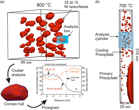
In Figure 8, the reconstructions of two APT tips after heat treatment at 800°C (Fig. 8a) and 700°C (Fig. 8b) are compared. The precipitates are visualized by isosurfaces (25 at.% Ni). Consistent with the results evaluated by TEM (see Fig. 7), the cooling precipitates are larger after heat treatment at 800°C. (The large precipitate also seen in Fig. 8b is part of a primary precipitate that exhibits a precipitate free zone around it.) In the reconstruction, the cooling precipitates have a lower atomic density than the matrix and appear compressed in the measurement direction when the specimen was cooled from 800°C (Fig. 8a). Surprisingly, after heat treatment at 700°C, they show the opposite behavior appearing more stretched in the measurement direction and have a higher atomic density (Fig. 8b and later Fig. 10). Since these precipitates naturally exhibit a spherical shape (cf. TEM images in Fig. 7) and are coherent to the matrix (with the same density), it is obvious that their APT reconstructions must have been influenced by local magnification artifacts, or possibly by a general erroneous scaling of the reconstruction, and therefore serve as an ideal example to test the presented model to evaluate the precipitates’ original sizes. Following the conclusions from the performed APT simulations, the precipitates reconstructed with a lower density after heat treatment at 800°C have a higher evaporation threshold than the matrix atoms (Φ FR > 1) and vice versa, after heat treatment at 700°C, precipitates are expected to have a lower evaporation threshold (Φ FR < 1).

Fig. 8. Reconstruction of two atom probe tips visualized by 25 at.% Ni isosurfaces after heat treatment of the alloy FBB-8 at 800°C (a) and 700°C (b); regions containing NiAl-type cooling precipitates (analyses boxes) were cropped to further study the cooling precipitates by cluster analysis and calculating proxigrams as shown in (a).
Precipitates with a Higher Evaporation Threshold than the Bulk
For the measurement represented in Figure 8a, five analysis boxes containing one precipitate each were cropped and further analyzed. First, the maximum separation method for cluster detection was applied for Ni atoms, allowing representation of the precipitate by a convex hull and calculation of the composition and density in the vicinity of the triangulated surface. As shown by the proxigram in Figure 8a, in this case of still rather large precipitates, a quantification of the fraction of Ni in the core of the precipitate (44 at.%) is best obtained by the fit with an error function (see also Table 1). On the contrary, the fraction of Ni would be underestimated, when calculating the Ni fraction from all atoms within the convex hull (33.5 at.%) because of a contribution of matrix atoms in the interface region.
Table 1. Comparison of the Evaluated Radii and Atomic Fractions of Ni Atoms of Five Different Precipitates after Heat Treatment at 800°C Obtained by Different Analysis Methods.

The isotropic radius R Exp(x, y, z) of each precipitate was then analyzed by the presented statistical approach (equation (5)) and applied to calculate the original radius R 0 by considering the density ratios Φ DR (equation (19)). From the number of excess atoms  ${\rm \Gamma }_B$, the density $\rho _{{\beta }^{\prime}}$, and the radius $R_{{\beta }^{\prime}}$ of the precipitate, the concentration of B atoms in the precipitate $c_{{\beta }^{\prime}}\;$can be calculated by
 $$c_{{\beta }^{\prime}} = \displaystyle{{{\rm \Gamma }_{\rm B}} \over {\rho _{{\beta }^{\prime}}\cdot ( 4/3) \pi R_{{\beta }^{\prime}}^3 }} + c_{0, B}, \;$$
where c 0,B is the concentration of solute atoms B in the matrix. Since the precipitates and matrix have the same density in the alloy FBB-8, the matrix density  $\rho _\alpha$ has to equal the density of the precipitates $\rho _{{\beta }^{\prime}}$ in the alloy. The obtained concentration $c_{{\beta }^{\prime}}$ is not reduced by the limited detection efficiency, since both the number of excess atoms ${\rm \Gamma }_B$ and the measured density $\rho _\alpha$ are reduced by the detection efficiency. On the other hand, the limited detection efficiency reduces the accuracy of the analysis, especially for small precipitates. Equation (20) can be applied to all elements which are enriched (show a positive excess) within the precipitate.
The concentration  $c_{{\beta }^{\prime}}$ can now be compared with the concentrations obtained from the proxigram and allows to cross-check, whether the size estimation was reasonable (cf. Table 1). In view of the data in the table, it becomes clear that both the size directly obtained from the convex hulls R CH, as well as the isotropic radius R Exp overestimate the real size of the precipitate. However, when using the observed density ratio for the calculation of the ratio in evaporation thresholds Φ FR by equation (18) (Φ DR = 1.14 ± 0.05) and applying this to calculate the original radii R 0 equation (19), the evaluated composition differs in average by only ±2.6 at.% Ni compared with the composition obtained from the proxigram. Consequently, the corrected size is convincingly close to the real size of the precipitate.
Precipitates with a Lower Evaporation Threshold than the Bulk
The second example (Fig. 8b) shows precipitates with a lower evaporation threshold that leads to a higher reconstructed density (see also Fig. 10). One cylinder over the complete width of the tip and with 37 nm in length containing 19 precipitates was cropped and further analyzed. After precipitate localization by cluster search and statistical size analysis of each individual cluster, the averaged isotropic mean radius R Exp of (1.45 ± 0.23) nm was determined. Applying equation (19), an original mean radius R 0 of (1.80 ± 0.31) nm with an average ratio in evaporation thresholds Φ FR of (0.83 ± 0.03) was calculated by considering the measured density ratios, which is very close to the radius evaluated by TEM, (1.7 ± 0.3) nm. Applying equation (20) to calculate the fraction of Ni in the precipitate yields a concentration of (73 ± 16) at.% Ni using the isotropic radius R Exp but (43.7 ± 7.0) at.% Ni when using the correctly calculated original radius R 0. The comparison of these concentrations to the average of (40.2 ± 2.1) at.% Ni obtained by evaluating all 19 proxigrams demonstrates the quality of the size corrected radius which only allows a realistic determination of the composition. Furthermore, this is a very clear example to demonstrate the impact of a small evaporation threshold on the volume of the reconstructed precipitate which is only half of the real volume of the precipitate.
Discussion
The presented examples have demonstrated that the original size of locally magnified or compressed precipitates in APT reconstructions can be correctly derived by considering the isotropic radii and the density ratios by equation (19). For the simulated tips in the section “Analysis of aspect ratios and relative density ratios”, it was shown that instead of the density ratios, also the aspect ratios equation (14) can be used for the calculation of the original precipitate radii. In this work, both methods to determine the original size of the precipitates have been tested with the result that the calculations using the density ratios performed better; especially for the large clusters presented in Figure 8a. The main reason for this is that the aspect ratio of the reconstructed precipitates depends very strongly on the quality of the APT reconstruction. A derivation of the assumed hemispherical tip shape, for example, due to crystallographic effects during reconstruction (Nakamura & Kuroda, Reference Nakamura and Kuroda1969; Waugh et al., Reference Waugh, Boyes and Southon1975; Oberdorfer & Schmitz, Reference Oberdorfer and Schmitz2011), modifies the reconstructed shape of the precipitates relative to the direction of a zone axis. Furthermore, the scaling of the z-dimension (measurement direction) of the APT tip depends on the field compression factor k f which is a user-defined parameter in the APT reconstruction protocol (Bas et al., Reference Bas, Bostel, Deconihout and Blavette1995). A common practice to derive this parameter is by tuning k f until either the geometry of (or the arrangement of features in) the APT reconstruction matches to the a priori known shape determined by correlative electron microscopy (Larson et al., Reference Larson, Russell and Miller1999; Arslan et al., Reference Arslan, Marquis, Homer, Hekmaty and Bartelt2008; De Geuser et al., Reference De Geuser, Gault, Stephenson, Moody and Muddle2008; Gault et al., Reference Gault, de Geuser, Bourgeois, Gabble, Ringer and Muddle2011a), or if visible, by matching the distance of reconstructed lattice planes with those in the real material (Gault et al., Reference Gault, Moody, Cairney and Ringer2012). If none of these methods can be applied, which was the case for the example shown in Figure 8a, a reconstruction with a correct in-depth scaling is so far not possible. Nonetheless, the size estimation of precipitates derived from the density ratios has shown to be a reliable measure of the evaporation thresholds of different species yielding accurate compositions, even if the in-depth scaling might not have been absolutely correct. A generalization of this approach to originally ellipsoidal (or other convex) shaped precipitates appears possible but still is to be tested in future studies.
In the APT reconstruction of the measurement performed with the voltage-pulsed atom probe (WATAP) (Fig. 8b), a better in-depth resolution was obtained and lattice planes became visible which are identified by the spatial distribution map (SDM) technique (Moody et al., Reference Moody, Gault, Stephenson, Haley and Ringer2009) in Figure 9a. Since 2D desorption maps have not revealed any clear zone axis or zone lines, an easy identification of the zone axis is not possible. Therefore, we performed several reconstructions with a variation in the field compression factor k f as presented in Figures 9b–9d and Figure 10, where k f was varied from 6.6 (a), to 7.6 (b), to 8.6 (c). In Figure 10, the atomic density of the reconstructed tips (left) and the triangulated convex hulls of precipitates after cluster search by the maximum separation method (right) are compared. The lattice plane distance can be extracted from small regions (4 × 4 × 6 nm3) around the zone axis by averaging the SDMs in the z-direction, as presented in Figures 9b–9d, and increases from 0.151 nm (b), to 0.205 nm (c), to 0.264 nm (d).

Fig. 9. (a) Spatial distribution map (SMD) in the x- and z-direction of atoms close to a zone axis in the sample heat treated at 700°C; (b–d) radial distribution maps obtained by averaging the SDM in the z-direction and applying different field compression factors kf of 6.6 (b), 7.6 (c), 8.6 (d) in the APT reconstruction. The data points were fitted by a sum of Gaussian functions.

Fig. 10. Density maps (left) and detected precipitates after use of the maximum separation algorithm and visualized by their triangulated convex hulls (right) of one APT dataset reconstructed by applying three different field compression factors kf of 6.6 (a), 7.6 (b), and 8.7 (c).
Based on the shown experimental data, there is seemingly no method to decide, which of the three APT reconstructions is best. Naively, one could choose the field compression factor k f (according to Fig. 10a), so that precipitates become spherical in the reconstruction and thereby ignoring local magnification effects. However, the more realistic solution can be found, when comparing the field ratio Φ FR obtained from the aspect ratios Φ AR (equation (13)) to the field ratio determined from the density ratios Φ DR (equation (18)), as shown in Table 2. Whereas Φ AR is strongly influenced by a variation in the field compression factor, Φ DR is constant for all three reconstructions and, therefore, is an independent measure of the field ratio Φ FR of ~0.83. Only for kf = 7.6, the field ratios obtained from Φ AR or Φ DR are equal, indicating that this field compression factor is the most realistic one. When comparing the evaluated lattice plane distances (see Figs. 9b–9d) to the theoretical distances in the bcc lattice of alloy FBB-8 (cf. Table 2), a distance of 0.2638 nm for kf = 8.6 is far off from any theoretical distance (d 110 = 0.2041 nm is the closest one) and also a distance of 0.1511 nm for kr = 6.6, does not clearly represent a specific lattice plane family in the ferritic alloy (d 111 = 0.1666 nm and d 200 = 0.1443 nm are closest). But for kr = 7.6, the measured lattice plane distance of 0.2045 nm agrees well with the distance of (110) planes (d 110 = 0.2041 nm). Furthermore, this field compression factor of 7.6 is confirmed when comparing the Ni concentration evaluated by equation (20) from the calculated radii of the precipitates (43.7 at.% by Φ AR and 43.4 at.% by Φ DR) to the concentration that is obtained by averaging all individual proxigrams (40.2 at.%). For kf = 6.6 and 8.6, the erroneously evaluated radius by the aspect ratios (1.75 or 2.02 nm, respectively) results in a strongly overestimated (84.6 at.% for kf = 6.6) or underestimated (26.6 at.% for kf = 8.6) amount in Ni. This example shows that the presented model for size evaluation of precipitates in APT datasets can be even applied to tune the field compression factor and, therefore, offers a new possibility to find the optimum in-depth scaling of APT measurements without prior knowledge of the APT tips shape and the visibility of lattice planes in the APT reconstruction.
Table 2. Analysis of the APT Measurement of the Sample Heat Treated at 700°C Reconstructed by Applying Three Different Field Compression Factors kf. Compared are the lattice plane distances evaluated by spatial distribution maps (SDM) and the closest theoretical lattice plane distance of the bcc Fe-alloy, the field ratios Φ FR derived by the aspect ratios Φ AR (equation (13)) and the density ratios Φ DR (equation (18)), the isotropic radius R Exp(x, y, z) and the calculated original radii R 0(Φ AR) (equation (14)) and R 0(Φ DR) (equation (19)) and the elemental concentration of Ni derived from the proxigrams and calculated with equation (20) applying the corrected radii estimates of the precipitates.

Conclusions
Numerical simulations were performed to study the influence of the field evaporation behavior of spherical nano-sized precipitates embedded in a matrix in APT measurements. A statistical analysis based on the evaluation of excess atoms of the precipitates revealed the following relations to the ratio in evaporation thresholds between the matrix and precipitate atoms:
• a linear relation with the isotropic radius derived from the gyration radius of the precipitates;
• a linear relation to the aspect ratio of the precipitates; and
• a quadratic relation to the cubic root of the density ratio of the precipitate and matrix densities.
With the observed relations, a model was developed to evaluate the original size of locally magnified or compressed precipitates. The model was tested on APT data of the ferritic alloy FBB-8 containing precipitates with either a higher (1.14 times) or lower (0.83 times) evaporation field compared with the surrounding bulk depending on the heat treatment. Complementary measurements by TEM and additional tests have shown that the size information after size correction with the proposed model are reliable.
Furthermore, it was shown that the proposed model can be used to tune the APT reconstruction parameters to find a correct in-depth scaling for cases where no lattice planes are visible in the APT reconstruction and no complementary information on the APT tip (shape) exists. It is also recommended as an independent method to evaluate the difference in evaporation thresholds of matrix and precipitates.
Supplementary material
To view supplementary material for this article, please visit https://doi.org/10.1017/S1431927621000180.
Acknowledgments
This work was supported by the German Research Foundation (grant numbers: SCHM 1182/19-2, HO 3322/3-1, WA 3818/1-1, and KR 3687/3-1). We thank Thomas Meisner and Arnold Weible for their assistance in the alloy fabrication, Daniel Beinke for the assistance in developing model datasets, and Sebastian Eich for the help on the spatial distribution mapping analysis.


 Open access