


1. Introduction
Two of the most prominent risk measures which are also extensively used in practice are Value at Risk and Conditional Tail Expectation. Both have their pros and cons and it is well known that Conditional Tail Expectation is the smallest coherent (in the sense of Artzner et al. Reference Artzner, Delbaen, Eber and Heath(1999)) risk measure dominating the Value at Risk (see e.g. Föllmer & Schied, Reference Föllmer and Schied2016: Theorem 4.67). Though in numerical examples the Conditional Tail Expectation is often much larger than the Value at Risk, given the same level  $\alpha$
. In this paper we present a class of risk measures which includes both the Value at Risk and the Conditional Tail Expectation. Another class with this property is the Range Value at Risk, introduced in Cont et al. (Reference Cont, Deguest and Scandolo2010) as a robustification of Value at Risk and Conditional Tail Expectation. Our approach relies on the generalisation of Quasi-Linear Means. Quasi-Linear Means can be traced back to Bonferroni (Reference Bonferroni1924: p. 103) who proposed a unifying formula for different means. Interestingly he motivated this with a problem from actuarial sciences about survival probabilities (for details see also Muliere & Parmigiani Reference Muliere and Parmigiani1993: p. 422).
$\alpha$
. In this paper we present a class of risk measures which includes both the Value at Risk and the Conditional Tail Expectation. Another class with this property is the Range Value at Risk, introduced in Cont et al. (Reference Cont, Deguest and Scandolo2010) as a robustification of Value at Risk and Conditional Tail Expectation. Our approach relies on the generalisation of Quasi-Linear Means. Quasi-Linear Means can be traced back to Bonferroni (Reference Bonferroni1924: p. 103) who proposed a unifying formula for different means. Interestingly he motivated this with a problem from actuarial sciences about survival probabilities (for details see also Muliere & Parmigiani Reference Muliere and Parmigiani1993: p. 422).
The Quasi-Linear Mean of a random variable X, denoted by  $\psi_{U}(X),$
is for an increasing, continuous function U defined as
$\psi_{U}(X),$
is for an increasing, continuous function U defined as
 \begin{equation*}
\psi_{U}\left(X\right) =U^{-1}\left( \mathbb{E}\left[ U\left( X\right)
\right] \right)
\label{eq11}
\end{equation*}
\begin{equation*}
\psi_{U}\left(X\right) =U^{-1}\left( \mathbb{E}\left[ U\left( X\right)
\right] \right)
\label{eq11}
\end{equation*}
where  $U^{-1}$
is the generalised inverse of U (see e.g. Muliere & Parmigiani, Reference Muliere and Parmigiani1993). If U is in addition concave,
$U^{-1}$
is the generalised inverse of U (see e.g. Muliere & Parmigiani, Reference Muliere and Parmigiani1993). If U is in addition concave,  $\psi_{U}(X)$
is a Certainty Equivalent. If U is convex
$\psi_{U}(X)$
is a Certainty Equivalent. If U is convex  $\psi_{U}(X)$
corresponds to the Mean Value Risk Measure (see Hardy et al., Reference Hardy, Littlewood and Polya1952). We take the actuarial point of view here, i.e. we assume that the random variable X is real-valued and represents a discounted net loss at the end of a fixed period. This means that positive values are losses whereas negative values are seen as gains. A well-known risk measure which is obtained when taking the exponential function in this definition is the Entropic Risk Measure which is known to be a convex risk measure but not coherent (see e.g. Müller, Reference Müller2007; Tsanakas, Reference Tsanakas2009).
$\psi_{U}(X)$
corresponds to the Mean Value Risk Measure (see Hardy et al., Reference Hardy, Littlewood and Polya1952). We take the actuarial point of view here, i.e. we assume that the random variable X is real-valued and represents a discounted net loss at the end of a fixed period. This means that positive values are losses whereas negative values are seen as gains. A well-known risk measure which is obtained when taking the exponential function in this definition is the Entropic Risk Measure which is known to be a convex risk measure but not coherent (see e.g. Müller, Reference Müller2007; Tsanakas, Reference Tsanakas2009).
In this paper, we generalise Quasi-Linear Means by focusing on the tail of the risk distribution. The proposed measure quantifies the Quasi-Linear Mean of an investor when conditioning on outcomes that are higher than its Value at Risk. More precisely it is defined by
 \begin{equation*}
\rho_{U}^{\alpha}(X)\,:\!=U^{-1}\Big(\mathbb{E}\big[U(X)|X\geq VaR_{\alpha
}(X)\big]\Big)
\end{equation*}
\begin{equation*}
\rho_{U}^{\alpha}(X)\,:\!=U^{-1}\Big(\mathbb{E}\big[U(X)|X\geq VaR_{\alpha
}(X)\big]\Big)
\end{equation*}
where  $VaR_{\alpha}$
is the usual Value at Risk. We call it Tail Quasi-Linear Mean (TQLM). It can be shown that when we restrict to concave (utility) functions, the TQLM interpolates between the Value at Risk and the Conditional Tail Expectation. By choosing the utility function U in the right way, we can be close to either the Value at Risk or the Conditional Tail Expectation. Both extreme cases are also included when we plug in specific utility functions. The Entropic Risk Measure is also a limiting case of our construction. Though in general not being convex, the TQLM has some nice properties. In particular, it is still manageable and useful in applications. We show the application of TQLM risk measures for capital allocation, for optimal reinsurance and for finding minimal risk portfolios. In particular, within the class of symmetric distributions we show that explicit computations lead to analytic closed-forms of TQLM.
$VaR_{\alpha}$
is the usual Value at Risk. We call it Tail Quasi-Linear Mean (TQLM). It can be shown that when we restrict to concave (utility) functions, the TQLM interpolates between the Value at Risk and the Conditional Tail Expectation. By choosing the utility function U in the right way, we can be close to either the Value at Risk or the Conditional Tail Expectation. Both extreme cases are also included when we plug in specific utility functions. The Entropic Risk Measure is also a limiting case of our construction. Though in general not being convex, the TQLM has some nice properties. In particular, it is still manageable and useful in applications. We show the application of TQLM risk measures for capital allocation, for optimal reinsurance and for finding minimal risk portfolios. In particular, within the class of symmetric distributions we show that explicit computations lead to analytic closed-forms of TQLM.
In the actuarial sciences there are already some approaches to unify risk measures or premium principles. Risk measures can be seen as a broader concept than insurance premium principles, since the latter one is considered as a “price” of a risk (for a discussion, see e.g. Goovaerts et al., Reference Goovaerts, Kaas, Dhaene and Tang2003; Furman & Zitikis, Reference Furman and Zitikis2008). Both are in its basic definition mappings from the space of random variables into the real numbers, but the interesting properties may vary with the application. In Goovaerts et al. (Reference Goovaerts, Kaas, Dhaene and Tang2003) a unifying approach to derive risk measures and premium principles has been proposed by minimising a Markov bound for the tail probability. The approach includes among others the Mean Value principle, the Swiss premium principle and Conditional Tail Expectation.
In Furman & Zitikis (Reference Furman and Zitikis2008), weighted premiums have been introduced where the expectation is taken with respect to a weighted distribution function. This construction includes e.g. the Conditional Tail Expectation, the Tail Variance and the Esscher premium. This paper also discusses invariance and additivity properties of these measures.
Further, the Mean Value Principle has been generalised in various ways. In Bühlmann et al. (Reference Bühlmann, Gagliardi, Gerber and Straub1977), these premium principles have been extended to the so-called Swiss Premium Principle which interpolates with the help of a parameter  $z\in[0,1]$
between the Mean Value Principle and the Zero-Utility Principle. Properties of the Swiss Premium Principle have been discussed in De Vylder & Goovaerts (Reference De Vylder and Goovaerts1980). In particular, monotonicity, positive subtranslativity and subadditivity for independent random variables are shown under some assumptions. The latter two notions are weakened versions of translation invariance and subadditivity, respectively.
$z\in[0,1]$
between the Mean Value Principle and the Zero-Utility Principle. Properties of the Swiss Premium Principle have been discussed in De Vylder & Goovaerts (Reference De Vylder and Goovaerts1980). In particular, monotonicity, positive subtranslativity and subadditivity for independent random variables are shown under some assumptions. The latter two notions are weakened versions of translation invariance and subadditivity, respectively.
The so-called Optimised Certainty Equivalent has been investigated in Ben-Tal & Teboulle (Reference Ben-Tal and Teboulle2007) as a mean to construct risk measures. It comprises the Conditional Tail Expectation and bounded shortfall risk.
The following section provides definitions and preliminaries on risk measures that will serve as necessary foundations for the paper. Section 3 introduces the proposed risk measure and derives its fundamental properties. We show various representations of this class of risk measures and prove for concave functions U (under a technical assumption) that the TQLM is bounded between the Value at Risk and the Conditional Tail Expectation. Unfortunately the only coherent risk measure in this class turns out to be the Conditional Tail Expectation (this is maybe not surprising since this is also true within the class of ordinary Certainty Equivalents, see Müller, Reference Müller2007). In Section 4 we consider the special case when we choose the exponential function. In this case we call  $\rho_U^\alpha$
Tail Conditional Entropic Risk Measure and show that it is convex within the class of comonotone random variables. Section 5 is devoted to applications. In the first part we discuss the application to capital allocation. We define a risk measure for each subportfolio based on our TQLM and discuss its properties. In the second part we consider an optimal reinsurance problem with the TQLM as target function. For convex functions U we show that the optimal reinsurance treaty is of stop-loss form. In Section 6, the proposed risk measure is investigated for the family of symmetric distributions. Some explicit calculations can be done there. In particular, there exists an explicit formula for the Tail Conditional Entropic Risk Measure. Finally, a minimal risk portfolio problem is solved when we consider the Tail Conditional Entropic Risk Measure as target function. Section 7 offers a discussion to the paper.
$\rho_U^\alpha$
Tail Conditional Entropic Risk Measure and show that it is convex within the class of comonotone random variables. Section 5 is devoted to applications. In the first part we discuss the application to capital allocation. We define a risk measure for each subportfolio based on our TQLM and discuss its properties. In the second part we consider an optimal reinsurance problem with the TQLM as target function. For convex functions U we show that the optimal reinsurance treaty is of stop-loss form. In Section 6, the proposed risk measure is investigated for the family of symmetric distributions. Some explicit calculations can be done there. In particular, there exists an explicit formula for the Tail Conditional Entropic Risk Measure. Finally, a minimal risk portfolio problem is solved when we consider the Tail Conditional Entropic Risk Measure as target function. Section 7 offers a discussion to the paper.
2. Classical Risk Measures and Other Preliminaries
We consider real-valued continuous random variables  $X\,:\, \Omega\to\mathbb{R}$
defined on a probability space
$X\,:\, \Omega\to\mathbb{R}$
defined on a probability space  $(\Omega, \mathcal{F},\mathbb{P})$
and denote this set by
$(\Omega, \mathcal{F},\mathbb{P})$
and denote this set by  $\mathcal{X}$
. These random variables represent discounted net losses at the end of a fixed period, i.e. positive values are seen as losses whereas negative values are seen as gains. We denote the (cumulative) distribution function by
$\mathcal{X}$
. These random variables represent discounted net losses at the end of a fixed period, i.e. positive values are seen as losses whereas negative values are seen as gains. We denote the (cumulative) distribution function by  $F_{X}(x)\,:\!=\mathbb{P}(X \leq
x), x\in\mathbb{R}$
. Moreover, we consider increasing and continuous functions
$F_{X}(x)\,:\!=\mathbb{P}(X \leq
x), x\in\mathbb{R}$
. Moreover, we consider increasing and continuous functions  $U\,:\,\mathbb{R}\to\mathbb{R}$
(in case X takes only positive or negative values, the domain of U can be restricted). The generalised inverse
$U\,:\,\mathbb{R}\to\mathbb{R}$
(in case X takes only positive or negative values, the domain of U can be restricted). The generalised inverse  $U^{-1}$
of such a function is defined by
$U^{-1}$
of such a function is defined by
 \begin{equation*}
U^{-1}(x)\,:\!=\inf\{y\in\mathbb{R}\,:\,U(y)\geq x\}
\end{equation*}
\begin{equation*}
U^{-1}(x)\,:\!=\inf\{y\in\mathbb{R}\,:\,U(y)\geq x\}
\end{equation*}
where  $x \in\mathbb{R}$
. With
$x \in\mathbb{R}$
. With
 \begin{equation*}
L^{1}\,:\!=\{X \in \mathcal{X}\,:\, \ X \text{ is a random variable with }
\mathbb{E}[X] < \infty\}
\end{equation*}
\begin{equation*}
L^{1}\,:\!=\{X \in \mathcal{X}\,:\, \ X \text{ is a random variable with }
\mathbb{E}[X] < \infty\}
\end{equation*}
we denote the space of all real-valued, continuous, integrable random variables. We now recall some notions of risk measures. In general, a risk measure is a mapping  $\rho\,:\, L^{1} \to\mathbb{R}\cup\{\infty\}$
. Of particular importance are the following risk measures.
$\rho\,:\, L^{1} \to\mathbb{R}\cup\{\infty\}$
. Of particular importance are the following risk measures.
Definition 2.1. For  $\alpha\in(0,1)$
and
$\alpha\in(0,1)$
and  $X \in L^{1}$
with distribution function
$X \in L^{1}$
with distribution function  $F_{X}$
we define
$F_{X}$
we define
(a) the Value at Risk of X at level $\alpha$
as
$VaR_{\alpha
}(X) \,:\!= \inf\{x\in\mathbb{R}\,:\, F_{X}(x)\geq\alpha\}$
,
$\alpha$
as
$VaR_{\alpha
}(X) \,:\!= \inf\{x\in\mathbb{R}\,:\, F_{X}(x)\geq\alpha\}$
,(b) the Conditional Tail Expectation of X at level
$\alpha$
as
\begin{equation*}
CTE_{\alpha}(X)\,:\!= \mathbb{E}[ X | X \ge VaR_{\alpha}(X)].
\end{equation*}


Note that for continuous random variables the definition of Conditional Tail Expectation is the same as the Average Value at Risk, the Expected Shortfall or the Tail Conditional Expectation (see Chapter 4 of Föllmer & Schied (Reference Föllmer and Schied2016) or Denuit et al. Reference Denuit, Dhaene, Goovaerts and Kaas(2006)). Below we summarise some properties of the generalised inverse (see e.g. McNeil et al., Reference McNeil, Frey and Embrechts2005: A.1.2).
Lemma 2.2. For an increasing, continuous function U with generalised inverse  $U^{-1}$
it holds the following:
$U^{-1}$
it holds the following:
(a)
$U^{-1}$
is strictly increasing and left-continuous.(b) For all
$x\in\mathbb{R}_{+}, y\in\mathbb{R}$
, we have
$U^{-1} \circ
U(x)\le x$
and
$U\circ U^{-1}(y) = y.$
(c) If U is strictly increasing on
$(x-\varepsilon,x)$
for an
$\varepsilon>0$
, we have
$U^{-1} \circ U(x)= x$
.


The next lemma is useful for alternative representations of our risk measure. It can be directly derived from the definition of Value at Risk.
Lemma 2.3. For  $\alpha\in(0,1)$
and any increasing, left-continuous function
$\alpha\in(0,1)$
and any increasing, left-continuous function  $f\,:\, \mathbb{R} \to\mathbb{R}$
it holds
$f\,:\, \mathbb{R} \to\mathbb{R}$
it holds  $VaR_{\alpha}(\kern1.5ptf(X)) =
f\big(VaR_{\alpha}(X)\big).$
$VaR_{\alpha}(\kern1.5ptf(X)) =
f\big(VaR_{\alpha}(X)\big).$
In what follows we will study some properties of risk measures  $\rho\,:\, L^{1} \to\mathbb{R}\cup\{\infty\}$
, like
$\rho\,:\, L^{1} \to\mathbb{R}\cup\{\infty\}$
, like
(i) law-invariance:
$\rho(X)$
depends only on the distribution
$F_{X}$
;(ii) constancy:
$\rho(m)=m$
for all
$m\in\mathbb{R}_{+}$
;(iii) monotonicity: if
$X\le Y$
, then
$\rho(X)\le\rho(Y)$
;(iv) translation invariance: for
$m\in\mathbb{R}$
, it holds
$\rho(X+m)=\rho(X)+m$
;(v) positive homogeneity: for
$\lambda\ge0$
it holds that
$\rho(\lambda X)=\lambda\rho(X);$
(vi) subadditivity:
$\rho(X+Y)\le\rho(X)+\rho(Y)$
;(vii) convexity: for
$\lambda\in[0,1]$
, it holds that
$\rho(\lambda X+(1-\lambda)Y)\le\lambda\rho(X)+(1-\lambda)\rho(Y).$


A risk measure with the properties (iii)–(vi) is called coherent. Note that  $CTE_{\alpha}(X)$
is not necessarily coherent when X is a discrete random variable, but is coherent if X is continuous. Also note that if
$CTE_{\alpha}(X)$
is not necessarily coherent when X is a discrete random variable, but is coherent if X is continuous. Also note that if  $\rho$
is positive homogeneous, then convexity and subadditivity are equivalent properties. Next we need the notion of the usual stochastic ordering (see e.g. Müller & Stoyan, Reference Müller and Stoyan2002).
$\rho$
is positive homogeneous, then convexity and subadditivity are equivalent properties. Next we need the notion of the usual stochastic ordering (see e.g. Müller & Stoyan, Reference Müller and Stoyan2002).
Definition 2.4. Let X,Y be two random variables. Then X is less than Y in usual stochastic order ( $X \leq_{st}Y$
) if
$X \leq_{st}Y$
) if  $\mathbb{E}[\kern1ptf(X)] \leq\mathbb{E}[\kern1ptf(Y)]$
for all increasing
$\mathbb{E}[\kern1ptf(X)] \leq\mathbb{E}[\kern1ptf(Y)]$
for all increasing  $f\,:\,\mathbb{R}\to\mathbb{R}$
, whenever the expectations exist. This is equivalent to
$f\,:\,\mathbb{R}\to\mathbb{R}$
, whenever the expectations exist. This is equivalent to  $F_{X}(t) \ge F_{Y}(t)$
for all
$F_{X}(t) \ge F_{Y}(t)$
for all  $t\in\mathbb{R}$
.
$t\in\mathbb{R}$
.
Finally we also have to deal with comonotone random variables (see e.g. Definition 1.9.1 in Denuit et al. Reference Denuit, Dhaene, Goovaerts and Kaas(2006));
Definition 2.5. Two random variables X, Y are called comonotone if there exists a random variable Z and increasing functions  $f,g\,:\,\mathbb{R}\to\mathbb{R}$
such that
$f,g\,:\,\mathbb{R}\to\mathbb{R}$
such that  $X=f(Z)$
and
$X=f(Z)$
and  $Y=g(Z)$
. The pair is called countermonotone if one of the two functions is increasing, the other decreasing.
$Y=g(Z)$
. The pair is called countermonotone if one of the two functions is increasing, the other decreasing.
3. Tail Quasi-Linear Means
For continuous random variables  $X\in \mathcal{X}$
and levels
$X\in \mathcal{X}$
and levels  $\alpha\in(0,1)$
let us introduce risk measures of the following form.
$\alpha\in(0,1)$
let us introduce risk measures of the following form.
Definition 3.1. Let  $X\in \mathcal{X}$
,
$X\in \mathcal{X}$
,  $\alpha\in (0,1)$
and U an increasing, continuous function. The TQLM is defined by
$\alpha\in (0,1)$
and U an increasing, continuous function. The TQLM is defined by
 \begin{equation}
\rho_{U}^{\alpha}(X)\,:\!=U^{-1}\Big(\mathbb{E}\big[U(X)|X\geq VaR_{\alpha
}(X)\big]\Big)
\label{eqn1}
\end{equation}
\begin{equation}
\rho_{U}^{\alpha}(X)\,:\!=U^{-1}\Big(\mathbb{E}\big[U(X)|X\geq VaR_{\alpha
}(X)\big]\Big)
\label{eqn1}
\end{equation}
whenever the conditional expectation inside exists and is finite.
(a) It is easy to see that
$U(x)=x$
leads to
$CTE_{\alpha}(X)$
.(b) The Quasi-Linear Mean
$\psi_U(X)$
is obtained by taking
$\lim_{\alpha\downarrow 0} \rho_U^\alpha(X).$


In what follows we will first give some alternative representations of the TQLM. By definition of the conditional distribution, it follows immediately that we can write
 \begin{equation*}
\rho_{U}^{\alpha}(X)= U^{-1}\left( \frac{\mathbb{E}\big[U(X) 1_{\{X\geq
VaR_{\alpha}(X)\}} \big]}{\mathbb{P}(X\ge VaR_{\alpha}(X))}\right)
\end{equation*}
\begin{equation*}
\rho_{U}^{\alpha}(X)= U^{-1}\left( \frac{\mathbb{E}\big[U(X) 1_{\{X\geq
VaR_{\alpha}(X)\}} \big]}{\mathbb{P}(X\ge VaR_{\alpha}(X))}\right)
\end{equation*}
where  $\mathbb{P}(X\ge VaR_{\alpha}(X))=1-\alpha$
for continuous X. Moreover, when we denote by
$\mathbb{P}(X\ge VaR_{\alpha}(X))=1-\alpha$
for continuous X. Moreover, when we denote by  $\tilde{\mathbb{P}}(\cdot)= \mathbb{P}(\cdot|
X\geq VaR_{\alpha}(X))$
the conditional probability given
$\tilde{\mathbb{P}}(\cdot)= \mathbb{P}(\cdot|
X\geq VaR_{\alpha}(X))$
the conditional probability given  $X\geq VaR_{\alpha
}(X)$
, then we obtain
$X\geq VaR_{\alpha
}(X)$
, then we obtain
 \begin{equation}\rho_{U}^{\alpha}(X)=U^{-1}\Big(\tilde{\mathbb{E}
}\big[U(X)\big]\Big)
\label{eqn2}
\end{equation}
\begin{equation}\rho_{U}^{\alpha}(X)=U^{-1}\Big(\tilde{\mathbb{E}
}\big[U(X)\big]\Big)
\label{eqn2}
\end{equation}
Thus,  $\rho_{U}^{\alpha}(X)$
is just the Quasi-Linear Mean of X with respect to the conditional distribution. In order to get an idea what the TQLM measures, suppose that U is sufficiently differentiable. Then we get by a Taylor series approximation (see e.g. Bielecki & Pliska, Reference Bielecki and Pliska2003) that
$\rho_{U}^{\alpha}(X)$
is just the Quasi-Linear Mean of X with respect to the conditional distribution. In order to get an idea what the TQLM measures, suppose that U is sufficiently differentiable. Then we get by a Taylor series approximation (see e.g. Bielecki & Pliska, Reference Bielecki and Pliska2003) that
 \begin{equation}
\rho_U^\alpha(X) \approx CTE_\alpha(X)-\frac12 \ell_U(CTE_\alpha(X)) TV_\alpha(X)
\label{eqn3}
\end{equation}
\begin{equation}
\rho_U^\alpha(X) \approx CTE_\alpha(X)-\frac12 \ell_U(CTE_\alpha(X)) TV_\alpha(X)
\label{eqn3}
\end{equation}
with  $\ell_U(x) = -\frac{U''(x)}{U'(x)}$
being the Arrow–Pratt function of absolute risk aversion and
$\ell_U(x) = -\frac{U''(x)}{U'(x)}$
being the Arrow–Pratt function of absolute risk aversion and
 \begin{equation}
TV_{\alpha}\left( X\right) \,:\!=Var\left( X|X\geq VaR_{\alpha}\left(X\right) \right) =
\mathbb{E}[(X-CTE_{\alpha}( X))^2 | X> VaR_\alpha(X)]
\label{eqn4}
\end{equation}
\begin{equation}
TV_{\alpha}\left( X\right) \,:\!=Var\left( X|X\geq VaR_{\alpha}\left(X\right) \right) =
\mathbb{E}[(X-CTE_{\alpha}( X))^2 | X> VaR_\alpha(X)]
\label{eqn4}
\end{equation}
being the tail variance of X. If U is concave  $\ell_U \ge 0$
and
$\ell_U \ge 0$
and  $TV_\alpha$
is subtracted from
$TV_\alpha$
is subtracted from  $CTE_\alpha$
. If U is convex
$CTE_\alpha$
. If U is convex  $\ell_U \le 0$
and
$\ell_U \le 0$
and  $TV_\alpha$
is added, penalising deviations in the tail. In this sense
$TV_\alpha$
is added, penalising deviations in the tail. In this sense  $\rho_U^\alpha(X) $
is approximately a Lagrange-function of a restricted optimisation problem, where we want to optimise the Conditional Tail Expectation under the restriction that the tail variance is not too high.
$\rho_U^\alpha(X) $
is approximately a Lagrange-function of a restricted optimisation problem, where we want to optimise the Conditional Tail Expectation under the restriction that the tail variance is not too high.
The following technical assumption will be useful:
(A) There exists an  $\varepsilon\gt0$
such that U is strictly increasing on
$\varepsilon\gt0$
such that U is strictly increasing on  $( VaR_{\alpha}(X) -\varepsilon,VaR_{\alpha}(X) )$
.
$( VaR_{\alpha}(X) -\varepsilon,VaR_{\alpha}(X) )$
.
Obviously assumption (A) is satisfied if U is strictly increasing on its domain which should be satisfied in all reasonable applications. Economically (A) states that at least shortly before the critical level  $VaR_{\alpha}(X)$
our measure strictly penalises higher outcomes of X. Under assumption (A) we obtain another representation of the TQLM.
$VaR_{\alpha}(X)$
our measure strictly penalises higher outcomes of X. Under assumption (A) we obtain another representation of the TQLM.
Lemma 3.3. For all  $X\in \mathcal{X}$
, increasing continuous functions U and
$X\in \mathcal{X}$
, increasing continuous functions U and  $\alpha\in(0,1)$
such that (A) is satisfied we have that
$\alpha\in(0,1)$
such that (A) is satisfied we have that
 \begin{equation*}
\rho_{U}^{\alpha}(X)=U^{-1}\Big( CTE_{\alpha}(U(X))\Big)
\end{equation*}
\begin{equation*}
\rho_{U}^{\alpha}(X)=U^{-1}\Big( CTE_{\alpha}(U(X))\Big)
\end{equation*}
Proof. We first show that under (A) we obtain
 \begin{equation*}
\{ X\ge VaR_{\alpha}(X)\} = \{ U(X)\ge VaR_{\alpha}(U(X))\}
\end{equation*}
\begin{equation*}
\{ X\ge VaR_{\alpha}(X)\} = \{ U(X)\ge VaR_{\alpha}(U(X))\}
\end{equation*}
Due to Lemma 2.3 we immediately obtain
 \begin{equation*}
\{ X\ge VaR_{\alpha}(X)\} \subset\{ U(X)\ge U(VaR_{\alpha}(X))\}=\{ U(X)\ge
VaR_{\alpha}(U(X))\}
\end{equation*}
\begin{equation*}
\{ X\ge VaR_{\alpha}(X)\} \subset\{ U(X)\ge U(VaR_{\alpha}(X))\}=\{ U(X)\ge
VaR_{\alpha}(U(X))\}
\end{equation*}
On the other hand, we have with Lemma 2.2 b),c) that
 \begin{equation*}
U(X)\ge VaR_{\alpha}(U(X)) \Rightarrow X\ge U^{-1} \circ U(X)\ge U^{-1} \circ
U(VaR_{\alpha}(X))=VaR_{\alpha}(X)
\end{equation*}
\begin{equation*}
U(X)\ge VaR_{\alpha}(U(X)) \Rightarrow X\ge U^{-1} \circ U(X)\ge U^{-1} \circ
U(VaR_{\alpha}(X))=VaR_{\alpha}(X)
\end{equation*}
which implies that both sets are equal.
Thus, we get that
 \begin{equation*}
\mathbb{E}\big[U(X)|X\geq VaR_{\alpha}(X)\big] = \mathbb{E}\big[U(X)|U(X)\geq
VaR_{\alpha}(U(X))\big] = CTE_{\alpha}(U(X))
\end{equation*}
\begin{equation*}
\mathbb{E}\big[U(X)|X\geq VaR_{\alpha}(X)\big] = \mathbb{E}\big[U(X)|U(X)\geq
VaR_{\alpha}(U(X))\big] = CTE_{\alpha}(U(X))
\end{equation*}
which implies the statement.
Next we provide some simple yet fundamental features of the TQLM. The first one is rather obvious and we skip the proof.
Lemma 3.4. For any  $ X \in \mathcal{X}$
, the TQLM and the Quasi-Linear Mean
$ X \in \mathcal{X}$
, the TQLM and the Quasi-Linear Mean  $\psi_{U}$
are related as follows:
$\psi_{U}$
are related as follows:
 \begin{equation*}
\rho_{U}^{\alpha}(X) \ge\psi_{U}(X)
\end{equation*}
\begin{equation*}
\rho_{U}^{\alpha}(X) \ge\psi_{U}(X)
\end{equation*}
The TQLM interpolates between the Value at Risk and the Conditional Tail Expectation in case U is concave. We will show this in the next theorem under our assumption (A) (see also Figure 1):
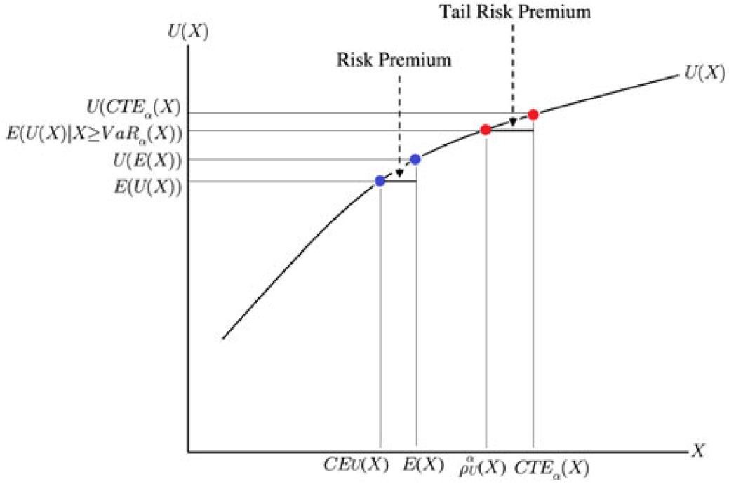
Figure 1. Relation between the TQLM, the CTE, the Certainty Equivalent and the expectation in case the utility function U is concave.
Theorem 3.5. For  $X\in \mathcal{X}$
and concave increasing functions U and
$X\in \mathcal{X}$
and concave increasing functions U and  $\alpha\in(0,1)$
such that (A) is satisfied, we have that
$\alpha\in(0,1)$
such that (A) is satisfied, we have that
 \begin{equation*}
VaR_{\alpha}(X) \le\rho_{U}^{\alpha}(X) \le CTE_{\alpha}(X)
\end{equation*}
\begin{equation*}
VaR_{\alpha}(X) \le\rho_{U}^{\alpha}(X) \le CTE_{\alpha}(X)
\end{equation*}
Moreover, there exist utility functions such that the bounds are attained. In case U is convex and satisfies (A) and all expectations exist, we obtain
 \begin{equation*}
\rho_{U}^{\alpha}(X) \ge CTE_{\alpha}(X)
\end{equation*}
\begin{equation*}
\rho_{U}^{\alpha}(X) \ge CTE_{\alpha}(X)
\end{equation*}
Proof. Let U be concave. We will first prove the upper bound. Here we use the representation of  $\rho_{U}^{\alpha}(X)$
in (2) as a Certainty Equivalent of the conditional distribution
$\rho_{U}^{\alpha}(X)$
in (2) as a Certainty Equivalent of the conditional distribution  $\tilde{\mathbb{P}}$
. We obtain with the Jensen inequality
$\tilde{\mathbb{P}}$
. We obtain with the Jensen inequality
 \begin{equation}\tilde{\mathbb{E}}[U(X)] \le U(\tilde{\mathbb{E}}[X]) =
U(CTE_{\alpha}(X))
\label{eqn5}
\end{equation}
\begin{equation}\tilde{\mathbb{E}}[U(X)] \le U(\tilde{\mathbb{E}}[X]) =
U(CTE_{\alpha}(X))
\label{eqn5}
\end{equation}
Taking the generalised inverse of U on both sides and using Lemma 2.2(a) and (b) yield
 \begin{equation*}
\rho_{U}^{\alpha}(X) \le U^{-1}\circ U(CTE_{\alpha}(X))\le CTE_{\alpha}(X)
\end{equation*}
\begin{equation*}
\rho_{U}^{\alpha}(X) \le U^{-1}\circ U(CTE_{\alpha}(X))\le CTE_{\alpha}(X)
\end{equation*}
The choice  $U(x)=x$
leads to
$U(x)=x$
leads to  $\rho_{U}^{\alpha}(X) =CTE_{\alpha}(X).$
For the lower bound first note that
 \begin{equation*}
U(VaR_{\alpha}(X))\leq\mathbb{E}\big[U(X)|X\geq VaR_{\alpha}(X)\big]
\end{equation*}
\begin{equation*}
U(VaR_{\alpha}(X))\leq\mathbb{E}\big[U(X)|X\geq VaR_{\alpha}(X)\big]
\end{equation*}
Taking the generalised inverse of U on both sides and using Lemma 2.2(c) yield
 \begin{equation*}
VaR_{\alpha}(X)=U^{-1}\circ U(VaR_{\alpha}(X))\leq\rho_{U}^{\alpha}(X)
\end{equation*}
\begin{equation*}
VaR_{\alpha}(X)=U^{-1}\circ U(VaR_{\alpha}(X))\leq\rho_{U}^{\alpha}(X)
\end{equation*}
Defining
 \begin{equation*}
U(x)=\left\{
\begin{array}[c]{cl}
x, & x\leq VaR_{\alpha}(X)\\
VaR_{\alpha}(X), & x>VaR_{\alpha}(X)
\end{array}
\right.
\end{equation*}
\begin{equation*}
U(x)=\left\{
\begin{array}[c]{cl}
x, & x\leq VaR_{\alpha}(X)\\
VaR_{\alpha}(X), & x>VaR_{\alpha}(X)
\end{array}
\right.
\end{equation*}
yields
 \begin{equation*}
U^{-1}(x)=\left\{
\begin{array}[c]{cl}
x, & x\leq VaR_{\alpha}(X)\\
\infty, & x>VaR_{\alpha}(X)
\end{array}
\right.
\end{equation*}
\begin{equation*}
U^{-1}(x)=\left\{
\begin{array}[c]{cl}
x, & x\leq VaR_{\alpha}(X)\\
\infty, & x>VaR_{\alpha}(X)
\end{array}
\right.
\end{equation*}
and we obtain
 \begin{equation*}
\mathbb{E}\big[U(X)|X\geq VaR_{\alpha}(X)\big]=U(VaR_{\alpha}(X))
\end{equation*}
\begin{equation*}
\mathbb{E}\big[U(X)|X\geq VaR_{\alpha}(X)\big]=U(VaR_{\alpha}(X))
\end{equation*}
Taking the generalised inverse of U on both sides and using Lemma 2.2(c) yield
 \begin{equation*}
\rho_{U}^{\alpha}(X)=U^{-1}\circ U(VaR_{\alpha}(X))=VaR_{\alpha}(X)
\end{equation*}
\begin{equation*}
\rho_{U}^{\alpha}(X)=U^{-1}\circ U(VaR_{\alpha}(X))=VaR_{\alpha}(X)
\end{equation*}
which shows that the lower bound can be attained. If U is convex, the inequality in (5) reverses.
Next we discuss the properties of the TQLM. Of course when we choose U in a specific way, we expect more properties to hold.
Theorem 3.6. The TQLM  $\rho_{U}^{\alpha}$
has the following properties:
$\rho_{U}^{\alpha}$
has the following properties:
(a) It is law-invariant.
(b) It has the constancy property.
(c) It is monotone.
(d) It is translation-invariant within the class of functions which are strictly increasing if and only if
$U(x)=-{\rm e}^{-\gamma x},\gamma
>0,$
or if U is linear.(e) It is positive homogeneous within the class of functions which are strictly increasing if and only
$U(x)=\frac{1}{\gamma}x^{\gamma
},x>0,\gamma\neq0$
or
$U(x)=\ln(x)$
or U is linear.

Proof.
(a) The law-invariance follows directly from the definition of
$\rho
_{U}^{\alpha}$
and the fact that
$VaR_{\alpha}$
is law-invariant.(b) For
$m\in\mathbb{R}$
we have that
$VaR_{\alpha}(m)=m$
and thus
$\tilde{\mathbb{P}}=\mathbb{P}$
which implies the statement.(c) We use here the representation
\begin{equation*}
\rho_{U}^{\alpha}(X)= U^{-1}\left( \frac{\mathbb{E}\big[U(X) 1_{\{X\geq
VaR_{\alpha}(X)\}} \big]}{1-\alpha}\right)
\end{equation*}
Thus it suffices to show that the relation
$X\le Y$
implies
$\mathbb{E}\big[U(X) 1_{\{X\geq
VaR_{\alpha}(X)\}} \big]\le \mathbb{E}\big[U(Y) 1_{\{Y\geq
VaR_{\alpha}(Y)\}} \big].$
Since we are only interested in the marginal distributions of X and Y, we can choose
$X=F_{X}^{-1}(V),Y=F_{Y}^{-1}(V)$
with same random variable V which is uniformly distributed on (0,1). We obtain with Lemma 2.2
\begin{align*}
& X\geq VaR_{\alpha}(X)\Leftrightarrow F_{X}^{-1}(V)\geq VaR_{\alpha}
(F_{X}^{-1}(V))\Leftrightarrow F_{X}^{-1}(V)\geq F_{X}^{-1}\big(VaR_{\alpha
}(V)\big)\\
& \Leftrightarrow F_{X}^{-1}(V)\geq F_{X}^{-1}\big(\alpha\big)\Leftrightarrow
V\geq\alpha
\end{align*}
The same holds true for Y. Since
$X\le Y$
, we obtain
$F_X^{-1} \le F_Y^{-1}$
, and thus
\begin{eqnarray*}
\mathbb{E}\big[U(X) 1_{\{X\geq VaR_{\alpha}(X)\}} \big] &=& \mathbb{E}\big[F_X^{-1}(V) 1_{\{V\geq \alpha\}} \big] \\ &\le& \mathbb{E}\big[F_Y^{-1}(V) 1_{\{V\geq \alpha\}} \big] = \mathbb{E}\big[U(Y) 1_{\{Y\geq VaR_{\alpha}(Y)\}} \big]
\end{eqnarray*}
which implies the result.
(d) Since we have the representation
(6)
\begin{equation}
\rho_{U}^{\alpha}(X)=U^{-1}\Big(\tilde{\mathbb{E}}\big[U(X)\big]\Big)
\label{eqn6}
\end{equation}
this statement follows from Müller (Reference Müller2007: Theorem 2.2). Note that we can work here with one fixed conditional distribution since
$\{X\ge VaR_{\alpha}(X)\}=\{X+c
\ge VaR_{\alpha}(X+c)\}$
for all
$c\in\mathbb{R}$
.(e) As in (d) this statement follows from Müller (Reference Müller2007: Theorem 2.3). Note that we can work here with one fixed conditional distribution since
$\{X\ge
VaR_{\alpha}(X)\}=\{\lambda X \ge VaR_{\alpha}(\lambda X)\}$
for all
$\lambda>0$
.


Remark 3.7. The monotonicity property of Theorem 3.6 seems to be obvious, but it indeed may not hold if X and Y are discrete. One has to be cautious in this case (see also the examples given in Bäuerle & Müller (Reference Bäuerle and Müller2006)). The same is true for the Conditional Tail Expectation.
Theorem 3.8. If  $\rho_{U}^{\alpha}$
is a coherent risk measure, then it is the Conditional Tail Expectation Measure
$\rho_{U}^{\alpha}$
is a coherent risk measure, then it is the Conditional Tail Expectation Measure  $\rho_{U}^{\alpha
}(X)=CTE_{\alpha}\left( X\right) .$
$\rho_{U}^{\alpha
}(X)=CTE_{\alpha}\left( X\right) .$
Proof. As can be seen from Theorem 3.6, the translation invariance and homogeneity properties hold simultaneously if and only if U is linear, which implies that  $\rho_{U}^{\alpha}$
is the Conditional Tail Expectation.
$\rho_{U}^{\alpha}$
is the Conditional Tail Expectation.
4. Tail Conditional Entropic Risk Measure
In case  $U(x)=\frac1\gamma {\rm e}^{\gamma x},\gamma\neq0,$
we obtain a conditional tail version of the Entropic Risk Measure. It is given by
$U(x)=\frac1\gamma {\rm e}^{\gamma x},\gamma\neq0,$
we obtain a conditional tail version of the Entropic Risk Measure. It is given by
 \begin{equation}
\rho_{U}^{\alpha}(X)=\frac{1}{\gamma}\log\mathbb{E}[{\rm e}^{\gamma X}|X\geq
VaR_{\alpha}(X)]
\label{eqn7}
\end{equation}
\begin{equation}
\rho_{U}^{\alpha}(X)=\frac{1}{\gamma}\log\mathbb{E}[{\rm e}^{\gamma X}|X\geq
VaR_{\alpha}(X)]
\label{eqn7}
\end{equation}
In this case we write  $\rho_{\gamma}^{\alpha}$
instead of
$\rho_{\gamma}^{\alpha}$
instead of  $\rho_{U}^{\alpha}$
, since U is determined by
$\rho_{U}^{\alpha}$
, since U is determined by  $\gamma$
. For
$\gamma$
. For  $\alpha\downarrow 0$
we obtain in the limit the classical Entropic Risk Measure. We call
$\alpha\downarrow 0$
we obtain in the limit the classical Entropic Risk Measure. We call  $\rho_{\gamma}^{\alpha}(X)$
Tail Conditional Entropic Risk Measure and get from (3) the following approximation of
$\rho_{\gamma}^{\alpha}(X)$
Tail Conditional Entropic Risk Measure and get from (3) the following approximation of  $\rho_{\gamma}^{\alpha}(X)$
: If
$\rho_{\gamma}^{\alpha}(X)$
: If  $\gamma\neq0$
is sufficiently close to zero, the conditional tail version of the Entropic Risk Measure can be approximated by
$\gamma\neq0$
is sufficiently close to zero, the conditional tail version of the Entropic Risk Measure can be approximated by
 \begin{equation*}
\rho_{\gamma}^{\alpha}(X)\approx CTE_{\alpha}\left( X\right) -\frac{\gamma
}{2}TV_{\alpha}\left( X\right)
\end{equation*}
\begin{equation*}
\rho_{\gamma}^{\alpha}(X)\approx CTE_{\alpha}\left( X\right) -\frac{\gamma
}{2}TV_{\alpha}\left( X\right)
\end{equation*}
i.e. it is a weighted measure consisting of Conditional Tail Expectation and Tail Variance (see (4)).
Another representation of the Tail Conditional Entropic Risk Measure is for  $\gamma\neq0$
given by (see e.g. Bäuerle & Rieder, Reference Bäuerle, Rieder and Piunovskiy2015; Ben-Tal & Teboulle, Reference Ben-Tal and Teboulle2007)
$\gamma\neq0$
given by (see e.g. Bäuerle & Rieder, Reference Bäuerle, Rieder and Piunovskiy2015; Ben-Tal & Teboulle, Reference Ben-Tal and Teboulle2007)
 \begin{equation*}
\rho_{\gamma}^{\alpha}(X)=\inf_{\mathbb{Q}\ll\tilde{\mathbb{P}}}\left(
\mathbb{E}_{\mathbb{Q}}[X]+\frac{1}{\gamma}\mathbb{E}_{\mathbb{Q}}\left(
\log\frac{d\mathbb{Q}}{d\tilde{\mathbb{P}}}\right) \right)
\end{equation*}
\begin{equation*}
\rho_{\gamma}^{\alpha}(X)=\inf_{\mathbb{Q}\ll\tilde{\mathbb{P}}}\left(
\mathbb{E}_{\mathbb{Q}}[X]+\frac{1}{\gamma}\mathbb{E}_{\mathbb{Q}}\left(
\log\frac{d\mathbb{Q}}{d\tilde{\mathbb{P}}}\right) \right)
\end{equation*}
where  $\tilde{\mathbb{P}}$
is again the conditional distribution
$\tilde{\mathbb{P}}$
is again the conditional distribution  $\mathbb{P}(\cdot|X\geq VaR_{\alpha}(X))$
. The minimising
$\mathbb{P}(\cdot|X\geq VaR_{\alpha}(X))$
. The minimising  ${\mathbb{Q}^{\ast}}$
is attained at
${\mathbb{Q}^{\ast}}$
is attained at
 \begin{equation*}
\mathbb{Q}^{\ast}(dz)=\frac{{\rm e}^{\gamma z}\tilde{\mathbb{P}}(dz)}{\int {\rm e}^{\gamma
y}\tilde{\mathbb{P}}(dy)}
\end{equation*}
\begin{equation*}
\mathbb{Q}^{\ast}(dz)=\frac{{\rm e}^{\gamma z}\tilde{\mathbb{P}}(dz)}{\int {\rm e}^{\gamma
y}\tilde{\mathbb{P}}(dy)}
\end{equation*}
According to Theorem 3.6, we cannot expect the Tail Conditional Entropic Risk Measure to be convex. However, we obtain the following result.
Theorem 4.1. For  $\gamma\gt0$
, the Tail Conditional Entropic Risk Measure is convex for comonotone random variables.
$\gamma\gt0$
, the Tail Conditional Entropic Risk Measure is convex for comonotone random variables.
Proof. First note that the Tail Conditional Entropic Risk Measure has the constancy property and is translation invariant. Thus, using Theorem 6 in Deprez & Gerber (Reference Deprez and Gerber1985) it is sufficient to show that  $g^{\prime\prime
}(0;\,X,Y)\geq0$
for all comonotone X,Y where
$g^{\prime\prime
}(0;\,X,Y)\geq0$
for all comonotone X,Y where
 \begin{equation*}
g(t;\,X,Y)=\rho_{\gamma}^{\alpha}(X+t(Y-X)),\quad t\in(0,1)
\end{equation*}
\begin{equation*}
g(t;\,X,Y)=\rho_{\gamma}^{\alpha}(X+t(Y-X)),\quad t\in(0,1)
\end{equation*}
Since X and Y are comonotone, we can write them as  $X=F_{X}^{-1}
(V),Y=F_{Y}^{-1}(V)$
with same random variable V which is uniformly distributed on (0,1). Thus we get with Lemma 2.2 (compare also the proof of Theorem 3.6(c))
$X=F_{X}^{-1}
(V),Y=F_{Y}^{-1}(V)$
with same random variable V which is uniformly distributed on (0,1). Thus we get with Lemma 2.2 (compare also the proof of Theorem 3.6(c))
 \begin{align*}
& X\geq VaR_{\alpha}(X)\Leftrightarrow F_{X}^{-1}(V)\geq VaR_{\alpha}
(F_{X}^{-1}(V))\Leftrightarrow F_{X}^{-1}(V)\geq F_{X}^{-1}\big(VaR_{\alpha
}(V)\big)\\
& \Leftrightarrow F_{X}^{-1}(V)\geq F_{X}^{-1}\big(\alpha\big)\Leftrightarrow
V\geq\alpha
\end{align*}
\begin{align*}
& X\geq VaR_{\alpha}(X)\Leftrightarrow F_{X}^{-1}(V)\geq VaR_{\alpha}
(F_{X}^{-1}(V))\Leftrightarrow F_{X}^{-1}(V)\geq F_{X}^{-1}\big(VaR_{\alpha
}(V)\big)\\
& \Leftrightarrow F_{X}^{-1}(V)\geq F_{X}^{-1}\big(\alpha\big)\Leftrightarrow
V\geq\alpha
\end{align*}
The same holds true for Y and also for  $X+t(Y-X)=(1-t)X+tY=(1-t)F_{X}
^{-1}(V)+tF_{Y}^{-1}(V)$
since it is an increasing, left-continuous function of V for
$X+t(Y-X)=(1-t)X+tY=(1-t)F_{X}
^{-1}(V)+tF_{Y}^{-1}(V)$
since it is an increasing, left-continuous function of V for  $t\in(0,1)$
. Thus all events on which we condition here are the same:
$t\in(0,1)$
. Thus all events on which we condition here are the same:
 \begin{equation*}
\{X\geq VaR_{\alpha}(X)\}\!=\!\{Y\geq VaR_{\alpha}(Y)\}\!=\!\{X+t(Y-X)\geq
VaR_{\alpha}(X+t(Y-X))\}\!=\!\{V\geq\alpha\}
\end{equation*}
\begin{equation*}
\{X\geq VaR_{\alpha}(X)\}\!=\!\{Y\geq VaR_{\alpha}(Y)\}\!=\!\{X+t(Y-X)\geq
VaR_{\alpha}(X+t(Y-X))\}\!=\!\{V\geq\alpha\}
\end{equation*}
Hence we obtain
 \begin{equation*}
g^{\prime}(t;\,X,Y)=\frac{\mathbb{E}\left[ (Y-X){\rm e}^{\gamma(X+t(Y-X))}
1_{[V\geq\alpha]}\right] }{\mathbb{E}\left[ {\rm e}^{\gamma(X+t(Y-X))}
1_{[V\geq\alpha]}\right] }
\end{equation*}
\begin{equation*}
g^{\prime}(t;\,X,Y)=\frac{\mathbb{E}\left[ (Y-X){\rm e}^{\gamma(X+t(Y-X))}
1_{[V\geq\alpha]}\right] }{\mathbb{E}\left[ {\rm e}^{\gamma(X+t(Y-X))}
1_{[V\geq\alpha]}\right] }
\end{equation*}
and
 \begin{equation*}
g^{\prime\prime}(0;\,X,Y)=\gamma\left\{ \frac{\mathbb{E}\left[ (Y-X)^{2}
{\rm e}^{\gamma X}1_{[V\geq\alpha]}\right] }{\mathbb{E}\left[ {\rm e}^{\gamma
X}1_{[V\geq\alpha]}\right] }-\left( \frac{\mathbb{E}\left[ (Y-X){\rm e}^{\gamma
X}1_{[V\geq\alpha]}\right] }{\mathbb{E}\left[ {\rm e}^{\gamma X}1_{[V\geq\alpha
]}\right] }\right) ^{2}\right\}
\end{equation*}
\begin{equation*}
g^{\prime\prime}(0;\,X,Y)=\gamma\left\{ \frac{\mathbb{E}\left[ (Y-X)^{2}
{\rm e}^{\gamma X}1_{[V\geq\alpha]}\right] }{\mathbb{E}\left[ {\rm e}^{\gamma
X}1_{[V\geq\alpha]}\right] }-\left( \frac{\mathbb{E}\left[ (Y-X){\rm e}^{\gamma
X}1_{[V\geq\alpha]}\right] }{\mathbb{E}\left[ {\rm e}^{\gamma X}1_{[V\geq\alpha
]}\right] }\right) ^{2}\right\}
\end{equation*}
This expression can be interpreted as the variance of  $(Y-X)$
under the probability measure
$(Y-X)$
under the probability measure
 \begin{equation*}
\frac{d\mathbb{P}^{\prime}}{d\mathbb{P}}=\frac{{\rm e}^{\gamma X}1_{[V\geq\alpha]}
}{\mathbb{E}\left[ {\rm e}^{\gamma X}1_{[V\geq\alpha]}\right] }
\end{equation*}
\begin{equation*}
\frac{d\mathbb{P}^{\prime}}{d\mathbb{P}}=\frac{{\rm e}^{\gamma X}1_{[V\geq\alpha]}
}{\mathbb{E}\left[ {\rm e}^{\gamma X}1_{[V\geq\alpha]}\right] }
\end{equation*}
and is thus greater or equal to zero which implies the statement.
5. Applications
In this section, we show that the TQLM is a useful tool for various applications in risk management.
5.1 Capital allocation
Firms often have the problem of allocating a global risk capital requirement down to subportfolios. One way to do this is to use Aumann–Shapley capital allocation rules. For convex risk measures, this is not an easy task and has e.g. been discussed in Tsanakas (Reference Tsanakas2009). A desirable property in this respect would be that the sum of the capital requirements for the subportfolios equals the global risk capital requirement. More precisely, let  $\left( X_{1},X_{2},\ldots,X_{n}\right) $
be a vector of n random variables and let
$\left( X_{1},X_{2},\ldots,X_{n}\right) $
be a vector of n random variables and let  $S=X_{1}+X_{2}+\cdots+X_{n}$
be its sum. An intuitive way to measure the contribution of
$S=X_{1}+X_{2}+\cdots+X_{n}$
be its sum. An intuitive way to measure the contribution of  $X_i$
to the total capital requirement, based on the TQLM, is by defining (compare for instance with Landsman & Valdez (Reference Landsman and Valdez2003)):
$X_i$
to the total capital requirement, based on the TQLM, is by defining (compare for instance with Landsman & Valdez (Reference Landsman and Valdez2003)):
 \begin{equation*}
\rho_{U}^{\alpha}\left( X_{i}|S\right) \,:\!=U^{-1}\left( \mathbb{E}\left[
U\left( X_{i}\right) |S\geq VaR_{\alpha}\left( S\right) \right] \right)
\end{equation*}
\begin{equation*}
\rho_{U}^{\alpha}\left( X_{i}|S\right) \,:\!=U^{-1}\left( \mathbb{E}\left[
U\left( X_{i}\right) |S\geq VaR_{\alpha}\left( S\right) \right] \right)
\end{equation*}
This results in a capital allocation rule if
 \begin{equation}
\rho_{U}^{\alpha}\left( S\right) =\sum_{i=1}^{n}\rho_{U}^{\alpha}\left(
X_{i}|S\right)
\label{eqn8}
\end{equation}
\begin{equation}
\rho_{U}^{\alpha}\left( S\right) =\sum_{i=1}^{n}\rho_{U}^{\alpha}\left(
X_{i}|S\right)
\label{eqn8}
\end{equation}
It is easily shown that this property is only true in a special case.
Theorem 5.1. The TQLM of the aggregated loss S is equal to the sum of TQLM of the risk sources  $X_{i},i=1,2,\ldots,n,$
i.e. (8) holds for all random variables
$X_{i},i=1,2,\ldots,n,$
i.e. (8) holds for all random variables  $X_{i},i=1,2,\ldots,n,$
if and only if U is linear.
$X_{i},i=1,2,\ldots,n,$
if and only if U is linear.
In general we cannot expect (8) to hold. Indeed for the Tail Conditional Entropic Risk Measure we obtain that in case the losses are comonotone, it is not profitable to split the portfolio in subportfolios, whereas it is profitable if two losses are countermonotone.
Theorem 5.2. The Tail Conditional Entropic Risk Measure has for  $\gamma\gt0$
and comonotone
$\gamma\gt0$
and comonotone  $X_i, i=1,\ldots, n$
the property that
$X_i, i=1,\ldots, n$
the property that
 \begin{equation*}
\rho^{\alpha}_{\gamma}(S) \ge\sum_{i=1}^{n} \rho_{\gamma}^{\alpha}(X_{i}|S)
\end{equation*}
\begin{equation*}
\rho^{\alpha}_{\gamma}(S) \ge\sum_{i=1}^{n} \rho_{\gamma}^{\alpha}(X_{i}|S)
\end{equation*}
In case  $n=2$
and
$n=2$
and  $X_1, X_2$
are countermonotone, the inequality reverses.
$X_1, X_2$
are countermonotone, the inequality reverses.
Proof. As in the proof of Theorem 4.1, we get for comonotone X,Y that  $X=F_{X}^{-1}(V), Y=F_{Y}^{-1}(V)$
with same random variable V which is uniformly distributed on (0,1) and that
$X=F_{X}^{-1}(V), Y=F_{Y}^{-1}(V)$
with same random variable V which is uniformly distributed on (0,1) and that
 \begin{align*}
& X+Y\geq VaR_{\alpha}(X+Y)\Leftrightarrow V\geq\alpha
\end{align*}
\begin{align*}
& X+Y\geq VaR_{\alpha}(X+Y)\Leftrightarrow V\geq\alpha
\end{align*}
Thus with  $S=X+Y$
 \begin{eqnarray*}
\frac{1}{1-\alpha}\mathbb{E}\Big[{\rm e}^{\gamma(X+Y)} 1_{[S\ge VaR_\alpha(S)]}\Big] &=& \frac{1}{1-\alpha} \mathbb{E}\Big[{\rm e}^{\gamma (F_X^{-1}(V)+F_Y^{-1}(V))} 1_{[V\ge \alpha]} \Big] \\
&=& \tilde{\mathbb{E}} \Big[ {\rm e}^{\gamma F_X^{-1}(V)} {\rm e}^{\gamma F_Y^{-1}(V)} \Big]\\
&\ge & \tilde{\mathbb{E}}\Big[{\rm e}^{\gamma F_X^{-1}(V)} \Big] \tilde{\mathbb{E}}\Big[ {\rm e}^{\gamma F_Y^{-1}(V)} \Big] \\
&=& \frac{1}{1-\alpha}\mathbb{E}\Big[{\rm e}^{\gamma X} 1_{[S\ge VaR_\alpha(S)]}\Big] \frac{1}{1-\alpha}\mathbb{E}\Big[{\rm e}^{\gamma Y} 1_{[S\ge VaR_\alpha(S)]}\Big]
\end{eqnarray*}
\begin{eqnarray*}
\frac{1}{1-\alpha}\mathbb{E}\Big[{\rm e}^{\gamma(X+Y)} 1_{[S\ge VaR_\alpha(S)]}\Big] &=& \frac{1}{1-\alpha} \mathbb{E}\Big[{\rm e}^{\gamma (F_X^{-1}(V)+F_Y^{-1}(V))} 1_{[V\ge \alpha]} \Big] \\
&=& \tilde{\mathbb{E}} \Big[ {\rm e}^{\gamma F_X^{-1}(V)} {\rm e}^{\gamma F_Y^{-1}(V)} \Big]\\
&\ge & \tilde{\mathbb{E}}\Big[{\rm e}^{\gamma F_X^{-1}(V)} \Big] \tilde{\mathbb{E}}\Big[ {\rm e}^{\gamma F_Y^{-1}(V)} \Big] \\
&=& \frac{1}{1-\alpha}\mathbb{E}\Big[{\rm e}^{\gamma X} 1_{[S\ge VaR_\alpha(S)]}\Big] \frac{1}{1-\alpha}\mathbb{E}\Big[{\rm e}^{\gamma Y} 1_{[S\ge VaR_\alpha(S)]}\Big]
\end{eqnarray*}
since the covariance is positive for comonotone random variables. Here, as before  $\tilde{\mathbb{P}}$
is the conditional distribution given by
$\tilde{\mathbb{P}}$
is the conditional distribution given by  $\frac{d\tilde{\mathbb{P}}}{d\mathbb{P}}=\frac{1}{1-\alpha} 1_{[V\ge \alpha]}$
. Taking
$\frac{d\tilde{\mathbb{P}}}{d\mathbb{P}}=\frac{1}{1-\alpha} 1_{[V\ge \alpha]}$
. Taking  $\frac{1}{\gamma} \log$
on both sides implies the result for
$\frac{1}{\gamma} \log$
on both sides implies the result for  $n=2$
. The general result follows by induction on the number of random variables. In the countermonotone case the inequality reverses.
$n=2$
. The general result follows by induction on the number of random variables. In the countermonotone case the inequality reverses.
5.2 Optimal reinsurance
TQLM risk measures can also be used to find optimal reinsurance treaties. In case the random variable X describes a loss, the insurance company is able to reduce its risk by splitting X into two parts and transferring one of these parts to a reinsurance company. More formally a reinsurance treaty is a function  $f\,:\,\mathbb{R}_{+}\to\mathbb{R}_{+}$
such that
$f\,:\,\mathbb{R}_{+}\to\mathbb{R}_{+}$
such that  $f(x)\le x$
and f as well as
$f(x)\le x$
and f as well as  $R_{f}(x) \,:\!= x-f(x)$
are both increasing. The reinsured part is then f(x). The latter assumption is often made to rule out moral hazard. In what follows let
$R_{f}(x) \,:\!= x-f(x)$
are both increasing. The reinsured part is then f(x). The latter assumption is often made to rule out moral hazard. In what follows let
 \begin{equation*}
\mathcal{C} = \{\kern1ptf\,:\,\mathbb{R}_{+} \to\mathbb{R}_{+} | \ f(x) \leq x \ \forall x
\in\mathbb{R}_{+} \text{ and } f, R_{f} \text{ are increasing}\}
\end{equation*}
\begin{equation*}
\mathcal{C} = \{\kern1ptf\,:\,\mathbb{R}_{+} \to\mathbb{R}_{+} | \ f(x) \leq x \ \forall x
\in\mathbb{R}_{+} \text{ and } f, R_{f} \text{ are increasing}\}
\end{equation*}
be the set of all reinsurance treaties. Note that functions in  $\mathcal{C}$
are in particular Lipschitz-continuous, since
$\mathcal{C}$
are in particular Lipschitz-continuous, since  $R_{f}$
increasing leads to
$R_{f}$
increasing leads to  $f(x_{2})-f(x_{1}) \le x_{2}-x_{1}$
for all
$f(x_{2})-f(x_{1}) \le x_{2}-x_{1}$
for all  $0\le x_{1}\le x_{2}$
. Of course the insurance company has to pay a premium to the reinsurer for taking part of the risk. For simplicity we assume here that the premium is computed according to the expected value premium principle, i.e. it is given by
$0\le x_{1}\le x_{2}$
. Of course the insurance company has to pay a premium to the reinsurer for taking part of the risk. For simplicity we assume here that the premium is computed according to the expected value premium principle, i.e. it is given by  $
(1+\theta)\mathbb{E}[f(X)]
$
for
$
(1+\theta)\mathbb{E}[f(X)]
$
for  $\theta\gt0$
and a certain amount
$\theta\gt0$
and a certain amount  $P\gt0$
is available for reinsurance. The aim is now to solve
$P\gt0$
is available for reinsurance. The aim is now to solve
 \begin{equation}\min_f\quad\rho_{U}^{\alpha}\big( R_{f}(X) \big) \quad
s.t.\quad(1+\theta) \mathbb{E}[\kern1ptf(X)] =P,\; f \in\mathcal{C}
\label{eqn9}
\end{equation}
\begin{equation}\min_f\quad\rho_{U}^{\alpha}\big( R_{f}(X) \big) \quad
s.t.\quad(1+\theta) \mathbb{E}[\kern1ptf(X)] =P,\; f \in\mathcal{C}
\label{eqn9}
\end{equation}
This means that the insurance company tries to minimise the retained risk, given the amount P is available for reinsurance. Problems like this can e.g. be found in Gajek & Zagrodny (Reference Gajek and Zagrodny2004). A multi-dimensional extension is given in Bäuerle & Glauner (Reference Bäuerle and Glauner2018). In what follows we assume that U is strictly increasing, strictly convex and continuously differentiable, i.e. according to (3) large deviations in the right tail of  $R_f(X)$
are heavily penalised. In order to avoid trivial cases, we assume that the available amount of money for reinsurance is not too high, i.e. we assume that
$R_f(X)$
are heavily penalised. In order to avoid trivial cases, we assume that the available amount of money for reinsurance is not too high, i.e. we assume that
 \begin{equation*}
P< (1+\theta)\mathbb{E}[ (X-VaR_{\alpha}(X))_{+}]
\end{equation*}
\begin{equation*}
P< (1+\theta)\mathbb{E}[ (X-VaR_{\alpha}(X))_{+}]
\end{equation*}
The optimal reinsurance treaty is given in the following theorem. It turns out to be a stop-loss treaty.
Theorem 5.3. The optimal reinsurance treaty of problem (9) is given by
 \begin{equation*}
f^{*}(x) = \left\{
\begin{array}[c]{cl}
0, & x \le a\\
x-a, & x\gt a
\end{array}
\right.
\end{equation*}
\begin{equation*}
f^{*}(x) = \left\{
\begin{array}[c]{cl}
0, & x \le a\\
x-a, & x\gt a
\end{array}
\right.
\end{equation*}
where a is a positive solution of  $
\left( 1+\theta \right)\mathbb{E}[{{(X-a)}_{+}}]=P.
$
$
\left( 1+\theta \right)\mathbb{E}[{{(X-a)}_{+}}]=P.
$
Note that the optimal reinsurance treaty does not depend on the precise form of U, i.e. on the precise risk aversion of the insurance company.
Proof. First observe that  $z \mapsto\mathbb{E}[ (X-z)_{+}]$
is continuous and decreasing. Moreover, by assumption
$z \mapsto\mathbb{E}[ (X-z)_{+}]$
is continuous and decreasing. Moreover, by assumption  $P< (1+\theta)\mathbb{E}[ (X-VaR_{\alpha}(X))_{+}].$
Thus by the mean-value theorem there exists an
$P< (1+\theta)\mathbb{E}[ (X-VaR_{\alpha}(X))_{+}].$
Thus by the mean-value theorem there exists an  $a> VaR_{\alpha}(X)$
such that
$a> VaR_{\alpha}(X)$
such that  $\left( 1+\theta \right)\mathbb{E}[{{(X-a)}_{+}}]=P.$
Since
$\left( 1+\theta \right)\mathbb{E}[{{(X-a)}_{+}}]=P.$
Since  $U^{-1}$
is increasing, problem (9) is equivalent to
$U^{-1}$
is increasing, problem (9) is equivalent to
 \begin{equation*}
\label{eq:ORP2}\min\quad\mathbb{E} \Big[ U(R_{f}(X)) 1_{[R_{f}(X)\ge
VaR_{\alpha}(R_{f}(X))]} \big] \quad s.t.\quad(1+\theta) \mathbb{E}[\kern1ptf(X)]
=P,\; f \in\mathcal{C}
\end{equation*}
\begin{equation*}
\label{eq:ORP2}\min\quad\mathbb{E} \Big[ U(R_{f}(X)) 1_{[R_{f}(X)\ge
VaR_{\alpha}(R_{f}(X))]} \big] \quad s.t.\quad(1+\theta) \mathbb{E}[\kern1ptf(X)]
=P,\; f \in\mathcal{C}
\end{equation*}
Since  $f\in\mathcal{C}$
we have by Lemma 2.3 that
$f\in\mathcal{C}$
we have by Lemma 2.3 that  $VaR_{\alpha
}(R_{f}(X))= R_{f}(VaR_{\alpha}(X))$
, and since
$VaR_{\alpha
}(R_{f}(X))= R_{f}(VaR_{\alpha}(X))$
, and since  $R_{f}$
is non-decreasing we obtain
$R_{f}$
is non-decreasing we obtain
 \begin{equation*}
\{ X\ge VaR_{\alpha}(X)\} \subset\{ R_{f}(X)\ge R_{f}(VaR_{\alpha}(X)) =
VaR_{\alpha}(R_{f}(X))\}
\end{equation*}
\begin{equation*}
\{ X\ge VaR_{\alpha}(X)\} \subset\{ R_{f}(X)\ge R_{f}(VaR_{\alpha}(X)) =
VaR_{\alpha}(R_{f}(X))\}
\end{equation*}
On the other hand, it is reasonable to assume that  $f(x) = 0$
for
$f(x) = 0$
for  $x\le
VaR_{\alpha}(X)$
since this probability mass does not enter the target function which implies that
$x\le
VaR_{\alpha}(X)$
since this probability mass does not enter the target function which implies that  $R_{f}(x) = x$
for
$R_{f}(x) = x$
for  $x\le VaR_{\alpha}(X)$
and thus
$x\le VaR_{\alpha}(X)$
and thus
 \begin{equation*}
\{ R_{f}(X)\ge R_{f}(VaR_{\alpha}(X)) = VaR_{\alpha}(R_{f}(X))\} \subset\{
X\ge VaR_{\alpha}(X)\}
\end{equation*}
\begin{equation*}
\{ R_{f}(X)\ge R_{f}(VaR_{\alpha}(X)) = VaR_{\alpha}(R_{f}(X))\} \subset\{
X\ge VaR_{\alpha}(X)\}
\end{equation*}
In total we have that
 \begin{equation*}
\{ R_{f}(X)\ge VaR_{\alpha}(R_{f}(X))\} = \{ X\ge VaR_{\alpha}(X)\}
\end{equation*}
\begin{equation*}
\{ R_{f}(X)\ge VaR_{\alpha}(R_{f}(X))\} = \{ X\ge VaR_{\alpha}(X)\}
\end{equation*}
Hence, we can equivalently consider the problem
 \begin{equation*}
\label{eq:ORP3}\min_f\quad\mathbb{E} \Big[ U(R_{f}(X)) 1_{[X\ge VaR_{\alpha
}(X)]} \big] \quad s.t.\quad(1+\theta) \mathbb{E}[\kern1ptf(X)] =P,\; f \in
\mathcal{C}
\end{equation*}
\begin{equation*}
\label{eq:ORP3}\min_f\quad\mathbb{E} \Big[ U(R_{f}(X)) 1_{[X\ge VaR_{\alpha
}(X)]} \big] \quad s.t.\quad(1+\theta) \mathbb{E}[\kern1ptf(X)] =P,\; f \in
\mathcal{C}
\end{equation*}
Next note that we have for any convex, differentiable function  $g\,:\,
\mathbb{R}_{+}\to\mathbb{R}_{+}$
that
$g\,:\,
\mathbb{R}_{+}\to\mathbb{R}_{+}$
that
 \begin{equation*}
g(x)-g(y) \ge g^{\prime}(y)(x-y), \quad x,y \ge0
\end{equation*}
\begin{equation*}
g(x)-g(y) \ge g^{\prime}(y)(x-y), \quad x,y \ge0
\end{equation*}
Now consider the function  $g(z) \,:\!= U(x-z) 1_{[x\ge VaR_{\alpha}(X)]}+\lambda
z$
for fixed
$g(z) \,:\!= U(x-z) 1_{[x\ge VaR_{\alpha}(X)]}+\lambda
z$
for fixed  $\lambda\,:\!= U^{\prime}(a)>0$
and fixed
$\lambda\,:\!= U^{\prime}(a)>0$
and fixed  $x\in\mathbb{R}_{+}$
. By our assumption g is convex and differentiable with derivative
$x\in\mathbb{R}_{+}$
. By our assumption g is convex and differentiable with derivative
 \begin{equation*}g^{\prime}(z)
= -U^{\prime}(x-z) 1_{[x\ge VaR_{\alpha}(X)]} + \lambda\end{equation*}
\begin{equation*}g^{\prime}(z)
= -U^{\prime}(x-z) 1_{[x\ge VaR_{\alpha}(X)]} + \lambda\end{equation*}
Let  $f^{*}$
be the reinsurance treaty defined in the theorem and
$f^{*}$
be the reinsurance treaty defined in the theorem and  $f\in\mathcal{C}$
any other admissible reinsurance treaty. Then
$f\in\mathcal{C}$
any other admissible reinsurance treaty. Then
 \begin{align*}
& \mathbb{E}\big[ U(X-f(X)) 1_{[X\ge VaR_{\alpha}(X)]} - U(X-f^{*}(X))
1_{[X\ge VaR_{\alpha}(X)]} + \lambda(\kern1.5ptf(X)-f^{*}(X)) \big] \ge\\
& \ge\mathbb{E}\Big[ \big( {-} U^{\prime}(X-f^*(X))1_{[X\ge VaR_{\alpha}(X)]} + \lambda\big)(\kern1.5ptf(X)-f^{*}(X)) \Big]
\end{align*}
\begin{align*}
& \mathbb{E}\big[ U(X-f(X)) 1_{[X\ge VaR_{\alpha}(X)]} - U(X-f^{*}(X))
1_{[X\ge VaR_{\alpha}(X)]} + \lambda(\kern1.5ptf(X)-f^{*}(X)) \big] \ge\\
& \ge\mathbb{E}\Big[ \big( {-} U^{\prime}(X-f^*(X))1_{[X\ge VaR_{\alpha}(X)]} + \lambda\big)(\kern1.5ptf(X)-f^{*}(X)) \Big]
\end{align*}
Rearranging the terms and noting that  $\mathbb{E}[\kern1ptf(X)]=\mathbb{E}[\kern1ptf^{*}(X)]$
, we obtain
$\mathbb{E}[\kern1ptf(X)]=\mathbb{E}[\kern1ptf^{*}(X)]$
, we obtain
 \begin{align*}
& \mathbb{E}\big[ U(X-f(X)) 1_{[X\ge VaR_{\alpha}(X)]} \big] + \mathbb{E}
\Big[ \big( U^{\prime}(X-f^*(X))1_{[X\ge VaR_{\alpha}(X)]} - \lambda\big) (\kern1.5ptf(X)-f^{*}(X))\Big] \ge\\
& \ge\mathbb{E}\big[ U(X-f^{*}(X)) 1_{[X\ge VaR_{\alpha}(X)]}\big]
\end{align*}
\begin{align*}
& \mathbb{E}\big[ U(X-f(X)) 1_{[X\ge VaR_{\alpha}(X)]} \big] + \mathbb{E}
\Big[ \big( U^{\prime}(X-f^*(X))1_{[X\ge VaR_{\alpha}(X)]} - \lambda\big) (\kern1.5ptf(X)-f^{*}(X))\Big] \ge\\
& \ge\mathbb{E}\big[ U(X-f^{*}(X)) 1_{[X\ge VaR_{\alpha}(X)]}\big]
\end{align*}
The statement follows when we can show that
 \begin{equation*}
\mathbb{E}\Big[ \big( U^{\prime}(X-f^*(X))1_{[X\ge VaR_{\alpha}(X)]} - \lambda\big) (\kern1.5ptf(X)-f^{*}(X)) \Big]\le0
\end{equation*}
\begin{equation*}
\mathbb{E}\Big[ \big( U^{\prime}(X-f^*(X))1_{[X\ge VaR_{\alpha}(X)]} - \lambda\big) (\kern1.5ptf(X)-f^{*}(X)) \Big]\le0
\end{equation*}
We can write
 \begin{align*}
& \mathbb{E}\Big[ \big( U^{\prime}(X-f^*(X))1_{[X\ge VaR_{\alpha}(X)]} - \lambda\big)
(\kern1.5ptf(X)-f^{*}(X)) \Big]\\
& = \mathbb{E}\big[ 1_{[X \ge a ]}\big( U^{\prime}(X-f^*(X))1_{[X\ge VaR_{\alpha}(X)]} - \lambda\big)
(\kern1.5ptf(X)-f^{*}(X)) \big]+\\
& + \mathbb{E}\big[ 1_{[X \lt a ]} \big( U^{\prime}(X-f^*(X))1_{[X\ge VaR_{\alpha}(X)]} - \lambda\big)
(\kern1.5ptf(X)-f^{*}(X)) \big]
\end{align*}
\begin{align*}
& \mathbb{E}\Big[ \big( U^{\prime}(X-f^*(X))1_{[X\ge VaR_{\alpha}(X)]} - \lambda\big)
(\kern1.5ptf(X)-f^{*}(X)) \Big]\\
& = \mathbb{E}\big[ 1_{[X \ge a ]}\big( U^{\prime}(X-f^*(X))1_{[X\ge VaR_{\alpha}(X)]} - \lambda\big)
(\kern1.5ptf(X)-f^{*}(X)) \big]+\\
& + \mathbb{E}\big[ 1_{[X \lt a ]} \big( U^{\prime}(X-f^*(X))1_{[X\ge VaR_{\alpha}(X)]} - \lambda\big)
(\kern1.5ptf(X)-f^{*}(X)) \big]
\end{align*}
In the first case we obtain for  $X\ge a$
by definition of
$X\ge a$
by definition of  $f^*$
and
$f^*$
and  $\lambda$
(note that
$\lambda$
(note that  $a\gt VaR_\alpha(X)$
):
$a\gt VaR_\alpha(X)$
):
 \begin{equation*}
U^{\prime}(X-f^*(X))1_{[X\ge VaR_{\alpha}(X)]} - \lambda=U^{\prime}(a)-\lambda=0
\end{equation*}
\begin{equation*}
U^{\prime}(X-f^*(X))1_{[X\ge VaR_{\alpha}(X)]} - \lambda=U^{\prime}(a)-\lambda=0
\end{equation*}
In the second case we obtain for  $X\lt a$
that
$X\lt a$
that  $f(X)-f^{*}(X)=f(X)\ge0$
and since
$f(X)-f^{*}(X)=f(X)\ge0$
and since  $U^{\prime}$
is increasing:
$U^{\prime}$
is increasing:
 \begin{equation*}
U^{\prime}(X-f^*(X))1_{[X\ge VaR_{\alpha}(X)]} - \lambda\le\lambda1_{[X\ge
VaR_{\alpha}(X)]} - \lambda\le0
\end{equation*}
\begin{equation*}
U^{\prime}(X-f^*(X))1_{[X\ge VaR_{\alpha}(X)]} - \lambda\le\lambda1_{[X\ge
VaR_{\alpha}(X)]} - \lambda\le0
\end{equation*}
Hence the statement is shown.
6. TQLM for Symmetric Loss Models
The symmetric family of distributions is well known to provide suitable distributions in finance and actuarial science. This family generalises the normal distribution into a framework of flexible distributions that are symmetric. We say that a real-valued random variable X has a symmetric distribution, if its probability density function takes the form
 \begin{equation}
f_{X}(x)=\frac{1}{\sigma}g\left( \frac{1}{2}\left( \frac{x-\mu}{\sigma
}\right) ^{2}\right) ,\quad x\in\mathbb{R}
\label{eqn10}
\end{equation}
\begin{equation}
f_{X}(x)=\frac{1}{\sigma}g\left( \frac{1}{2}\left( \frac{x-\mu}{\sigma
}\right) ^{2}\right) ,\quad x\in\mathbb{R}
\label{eqn10}
\end{equation}
where  $g\left( t\right) \geq0,$ $t\geq0,$
is the density generator of X and satisfies
$t\geq0,$
is the density generator of X and satisfies
 \begin{equation*}
\int\limits_{0}^{\infty}t^{-1/2}g(t)dt<\infty
\end{equation*}
\begin{equation*}
\int\limits_{0}^{\infty}t^{-1/2}g(t)dt<\infty
\end{equation*}
The parameters  $\mu\in\mathbb{R}$
and
$\mu\in\mathbb{R}$
and  $\sigma^{2}\gt0$
are the expectation and the scale parameter of the distribution, respectively, and we write
$\sigma^{2}\gt0$
are the expectation and the scale parameter of the distribution, respectively, and we write  $X\sim {{S}_{1}}\left( \mu ,{{\sigma }^{2}},g \right)$
. If the variance of X exists, then it takes the form
$X\sim {{S}_{1}}\left( \mu ,{{\sigma }^{2}},g \right)$
. If the variance of X exists, then it takes the form
 \begin{equation*}
\mathbb{V}\left( X\right) =\sigma_{Z}^{2}\sigma^{2}
\end{equation*}
\begin{equation*}
\mathbb{V}\left( X\right) =\sigma_{Z}^{2}\sigma^{2}
\end{equation*}
where
 \begin{equation*}
\sigma_{Z}^{2}=2\underset{0}{\overset{\infty}{\int}}t^{2}g\left( \frac{1}
{2}t^{2}\right) dt<\infty
\end{equation*}
\begin{equation*}
\sigma_{Z}^{2}=2\underset{0}{\overset{\infty}{\int}}t^{2}g\left( \frac{1}
{2}t^{2}\right) dt<\infty
\end{equation*}
For the sequel, we also define the standard symmetric random variable  $
Z\sim {{S}_{1}}\left( 0,1,g \right)
$
and a cumulative generator
$
Z\sim {{S}_{1}}\left( 0,1,g \right)
$
and a cumulative generator  $\skew2\overline{G}(t),$
first defined in Landsman & Valdez (Reference Landsman and Valdez2003), that takes the form
$\skew2\overline{G}(t),$
first defined in Landsman & Valdez (Reference Landsman and Valdez2003), that takes the form
 \begin{equation*}\skew2\overline{G}
(t)=\underset{t}{\overset{\infty}{\int}}g(v)dv\end{equation*}
\begin{equation*}\skew2\overline{G}
(t)=\underset{t}{\overset{\infty}{\int}}g(v)dv\end{equation*}
with the condition  $\skew2\overline{G}(0)<\infty.$
Special members of the family of symmetric distributions are as follows:
$\skew2\overline{G}(0)<\infty.$
Special members of the family of symmetric distributions are as follows:
(a) The normal distribution,
$g(u)={\rm e}^{-u}/\sqrt{2\pi},$
(b) Student’s t-distribution
$g(u)=\frac{\Gamma(\frac{m+1}{2})}
{\Gamma(m/2)\sqrt{m\pi}}\left( 1+\frac{2u}{m}\right) ^{-\left( m+1\right)
/2}$
with
$m\gt0$
degrees of freedom,(c) Logistic distribution, with
$g\left( u\right) =c{\rm e}^{-u}/\left(
1+{\rm e}^{-u}\right) ^{2}$
where
$c\gt0$
is the normalising constant.


In what follows, we will consider the TQLM for this class of random variables.
Theorem 6.1. Let  $X\sim {{S}_{1}}(\mu ,{{\sigma }^{2}},g)$
. Then, the TQLM takes the following form
$X\sim {{S}_{1}}(\mu ,{{\sigma }^{2}},g)$
. Then, the TQLM takes the following form
 \begin{equation}
\rho_{U}^{\alpha}(X)=\rho_{\skew3\tilde{U}}^{\alpha}(Z)
\label{eqn11}
\end{equation}
\begin{equation}
\rho_{U}^{\alpha}(X)=\rho_{\skew3\tilde{U}}^{\alpha}(Z)
\label{eqn11}
\end{equation}
where  $\skew3\tilde{U}(x)=U(\sigma x+\mu).$
Proof. For the symmetric distributed X, we have
 \begin{equation*}
\rho_{U}^{\alpha}(X)= U^{-1}\left( \frac{\mathbb{E}\big[U(X) 1_{\{X\geq
VaR_{\alpha}(X)\}} \big]}{1-\alpha}\right)
\end{equation*}
\begin{equation*}
\rho_{U}^{\alpha}(X)= U^{-1}\left( \frac{\mathbb{E}\big[U(X) 1_{\{X\geq
VaR_{\alpha}(X)\}} \big]}{1-\alpha}\right)
\end{equation*}
Now we obtain
 \begin{align*}
\mathbb{E}\big[U(X) 1_{\{X\geq VaR_{\alpha}(X)\}} \big] & = \int
_{VaR_{\alpha}(X)}^{\infty}U(x) \frac{1}{\sigma} g\left(\frac12\left((\frac{x-\mu
}{\sigma}\right)^{2}\right)dx\\
& = \int_{\frac{VaR_{\alpha}(X)-\mu}{\sigma}}^{\infty}U(\sigma z+\mu)
g\left(\frac12 z^{2}\right)dz = \int_{VaR_{\alpha}(Z)}^{\infty}\skew3\tilde{U}(z) g\left(\frac12
z^{2}\right)dz\\
& = \mathbb{E}\big[\skew3\tilde{U}(Z) 1_{\{Z\geq VaR_{\alpha}(Z)\}} \big]
\end{align*}
\begin{align*}
\mathbb{E}\big[U(X) 1_{\{X\geq VaR_{\alpha}(X)\}} \big] & = \int
_{VaR_{\alpha}(X)}^{\infty}U(x) \frac{1}{\sigma} g\left(\frac12\left((\frac{x-\mu
}{\sigma}\right)^{2}\right)dx\\
& = \int_{\frac{VaR_{\alpha}(X)-\mu}{\sigma}}^{\infty}U(\sigma z+\mu)
g\left(\frac12 z^{2}\right)dz = \int_{VaR_{\alpha}(Z)}^{\infty}\skew3\tilde{U}(z) g\left(\frac12
z^{2}\right)dz\\
& = \mathbb{E}\big[\skew3\tilde{U}(Z) 1_{\{Z\geq VaR_{\alpha}(Z)\}} \big]
\end{align*}
where  $\skew3\tilde{U}(x)=U(\sigma x+\mu).$
Hence the statement follows.
$\skew3\tilde{U}(x)=U(\sigma x+\mu).$
Hence the statement follows.
For the special case of Tail Conditional Entropic Risk Measures, we obtain the following result.
Theorem 6.2. Let  $X\sim {{S}_{1}}(\mu ,{{\sigma }^{2}},g)$
. The moment generating function of X exists if and only if the Tail Conditional Entropic Risk Measure satisfies
$X\sim {{S}_{1}}(\mu ,{{\sigma }^{2}},g)$
. The moment generating function of X exists if and only if the Tail Conditional Entropic Risk Measure satisfies
 \begin{equation*}
\rho_{\gamma}^\alpha(X)=\mu+\sigma\rho_{\sigma\gamma}^\alpha(Z) \lt\infty
\end{equation*}
\begin{equation*}
\rho_{\gamma}^\alpha(X)=\mu+\sigma\rho_{\sigma\gamma}^\alpha(Z) \lt\infty
\end{equation*}
Proof. For a function U, we obtain:
 \begin{align*}
\mathbb{E}\Big[U(X)1_{[X\geq VaR_{\alpha}(X)]}\Big] & =\int_{VaR_{\alpha
}(X)}^{\infty}U(x)\frac{1}{\sigma}g\left(\frac{1}{2}\left(\frac{x-\mu}{\sigma}
\right)^{\!2}\right)dx\\
& =\int_{\frac{VaR_{\alpha}(X)-\mu}{\sigma}}^{\infty}U(\sigma y+\mu
)g\left(\frac{1}{2}y^{2}\right)dy
\end{align*}
\begin{align*}
\mathbb{E}\Big[U(X)1_{[X\geq VaR_{\alpha}(X)]}\Big] & =\int_{VaR_{\alpha
}(X)}^{\infty}U(x)\frac{1}{\sigma}g\left(\frac{1}{2}\left(\frac{x-\mu}{\sigma}
\right)^{\!2}\right)dx\\
& =\int_{\frac{VaR_{\alpha}(X)-\mu}{\sigma}}^{\infty}U(\sigma y+\mu
)g\left(\frac{1}{2}y^{2}\right)dy
\end{align*}
Plugging in  $U(x)=\frac1\gamma {\rm e}^{\gamma x}$
yields
$U(x)=\frac1\gamma {\rm e}^{\gamma x}$
yields
 \begin{equation*}
\mathbb{E}\Big[U(X)1_{[X\geq VaR_{\alpha}(X)]}\Big]=\frac1\gamma {\rm e}^{\gamma\mu}\int
_{\frac{VaR_{\alpha}(X)-\mu}{\sigma}}^{\infty}{\rm e}^{\gamma\sigma y}g\left(\frac{1}
{2}y^{2}\right)dy
\end{equation*}
\begin{equation*}
\mathbb{E}\Big[U(X)1_{[X\geq VaR_{\alpha}(X)]}\Big]=\frac1\gamma {\rm e}^{\gamma\mu}\int
_{\frac{VaR_{\alpha}(X)-\mu}{\sigma}}^{\infty}{\rm e}^{\gamma\sigma y}g\left(\frac{1}
{2}y^{2}\right)dy
\end{equation*}
Hence it follows that
 \begin{align*}
\rho_{\gamma}^\alpha(X) & =\frac{1}{\gamma}\Big\{\gamma\mu+\log\Big(\int
_{\frac{VaR_{\alpha}(X)-\mu}{\sigma}}^{\infty}{\rm e}^{\gamma\sigma y}g\Big(\frac{1}
{2}y^{2}\Big)dy\Big)-\log(1-\alpha)\Big\}\\
& =\mu+\sigma\frac{1}{\gamma\sigma}\log\Big(\int_{VaR_{\alpha}(Z)}^{\infty
}{\rm e}^{\gamma\sigma y}g\Big(\frac{1}{2}y^{2}\Big)dy\Big)+\sigma\frac{\log(1-\alpha
)}{\sigma\gamma}\\
& =\mu+\sigma\rho_{\sigma\gamma}^\alpha(Z)
\end{align*}
\begin{align*}
\rho_{\gamma}^\alpha(X) & =\frac{1}{\gamma}\Big\{\gamma\mu+\log\Big(\int
_{\frac{VaR_{\alpha}(X)-\mu}{\sigma}}^{\infty}{\rm e}^{\gamma\sigma y}g\Big(\frac{1}
{2}y^{2}\Big)dy\Big)-\log(1-\alpha)\Big\}\\
& =\mu+\sigma\frac{1}{\gamma\sigma}\log\Big(\int_{VaR_{\alpha}(Z)}^{\infty
}{\rm e}^{\gamma\sigma y}g\Big(\frac{1}{2}y^{2}\Big)dy\Big)+\sigma\frac{\log(1-\alpha
)}{\sigma\gamma}\\
& =\mu+\sigma\rho_{\sigma\gamma}^\alpha(Z)
\end{align*}
Also note that  $\rho_\gamma^\alpha(X)\lt\infty$
is equivalent to the existence of the moment generating function.
$\rho_\gamma^\alpha(X)\lt\infty$
is equivalent to the existence of the moment generating function.
In the following theorem, we derive an explicit formula for the Tail Conditional Entropic Risk Measure for the family of symmetric loss models. For this, we denote the cumulant function of Z by  $\kappa\left( t\right)
\,:\!=\log\psi\left( -\frac{1}{2}t^{2}\right)$
, where
$\kappa\left( t\right)
\,:\!=\log\psi\left( -\frac{1}{2}t^{2}\right)$
, where  $\psi$
is the characteristic generator, i.e. it satisfies
$\psi$
is the characteristic generator, i.e. it satisfies  $\mathbb{E}[{\rm e}^{itX}]= {\rm e}^{it\mu} \psi(\frac12 t^2\sigma^2).$
Theorem 6.3. Let  $X\sim {{S}_{1}}(\mu ,{{\sigma }^{2}},g)$
and assume that the moment generating function of X exists. Then the Tail Conditional Entropic Risk Measure is given by
$X\sim {{S}_{1}}(\mu ,{{\sigma }^{2}},g)$
and assume that the moment generating function of X exists. Then the Tail Conditional Entropic Risk Measure is given by
 \begin{equation*}
\rho_{\gamma}^\alpha(X)=\mu+\gamma^{-1}\kappa\left( \gamma\sigma\right)
+\log\left( \frac{\skew2\overline{F}_{Y}\left( VaR_{\alpha}\left( Z\right)
\right) }{1-\alpha}\right) ^{-1/\gamma}
\end{equation*}
\begin{equation*}
\rho_{\gamma}^\alpha(X)=\mu+\gamma^{-1}\kappa\left( \gamma\sigma\right)
+\log\left( \frac{\skew2\overline{F}_{Y}\left( VaR_{\alpha}\left( Z\right)
\right) }{1-\alpha}\right) ^{-1/\gamma}
\end{equation*}
Here  $F_{Y}\left( y\right) $
is the cumulative distribution function of a random variable Y with the density
$F_{Y}\left( y\right) $
is the cumulative distribution function of a random variable Y with the density
 \begin{equation*}
f_{Y}\left( y\right) =\frac{{\rm e}^{\gamma\sigma y}}{\psi\left( -\frac{1}
{2}\gamma^{2}\sigma^{2}\right) }g\left( \frac{1}{2}y^{2}\right)
,y\in\mathbb{R}
\end{equation*}
\begin{equation*}
f_{Y}\left( y\right) =\frac{{\rm e}^{\gamma\sigma y}}{\psi\left( -\frac{1}
{2}\gamma^{2}\sigma^{2}\right) }g\left( \frac{1}{2}y^{2}\right)
,y\in\mathbb{R}
\end{equation*}
and  $\skew2\overline{F}_{Y}$
is its tail distribution function.
$\skew2\overline{F}_{Y}$
is its tail distribution function.
Proof. From the previous theorem, we have that  $\rho_{\gamma}^\alpha(X)=\mu+\sigma
\rho_{\sigma\gamma}^\alpha(Z)$
, where
$\rho_{\gamma}^\alpha(X)=\mu+\sigma
\rho_{\sigma\gamma}^\alpha(Z)$
, where  $Z\sim {{S}_{1}}(0,1,g).$
Then, from Landsman et al. (Reference Landsman, Makov and Shushi2016), the conditional characteristic function of the symmetric distribution can be calculated explicitly, as follows:
$Z\sim {{S}_{1}}(0,1,g).$
Then, from Landsman et al. (Reference Landsman, Makov and Shushi2016), the conditional characteristic function of the symmetric distribution can be calculated explicitly, as follows:
 \begin{equation*}
\mathbb{E}\left[ {\rm e}^{\gamma\sigma Z}|Z\geq VaR_{\alpha}\left( Z\right)
\right] =\frac{\int\limits_{VaR_{\alpha}\left( Z\right) }^{\infty
}{\rm e}^{\gamma\sigma z}g\left( \frac{1}{2}z^{2}\right) dz}{1-\alpha}
\end{equation*}
\begin{equation*}
\mathbb{E}\left[ {\rm e}^{\gamma\sigma Z}|Z\geq VaR_{\alpha}\left( Z\right)
\right] =\frac{\int\limits_{VaR_{\alpha}\left( Z\right) }^{\infty
}{\rm e}^{\gamma\sigma z}g\left( \frac{1}{2}z^{2}\right) dz}{1-\alpha}
\end{equation*}
Observing that the following relation holds for any characteristic generator  $\psi$
of g (see, for instance Landsman et al., Reference Landsman, Makov and Shushi2016; Dhaene et al., Reference Dhaene, Henrard, Landsman, Vandendorpe and Vanduffel2008)
$\psi$
of g (see, for instance Landsman et al., Reference Landsman, Makov and Shushi2016; Dhaene et al., Reference Dhaene, Henrard, Landsman, Vandendorpe and Vanduffel2008)
 \begin{equation*}
\int\limits_{-\infty}^{a}{\rm e}^{\gamma\sigma z}g\left( \frac{1}{2}z^{2}\right)
dz=\psi\left( -\frac{1}{2}\gamma^{2}\sigma^{2}\right) F_{Y}\left(a\right)\!,a\in\mathbb{R}
\end{equation*}
\begin{equation*}
\int\limits_{-\infty}^{a}{\rm e}^{\gamma\sigma z}g\left( \frac{1}{2}z^{2}\right)
dz=\psi\left( -\frac{1}{2}\gamma^{2}\sigma^{2}\right) F_{Y}\left(a\right)\!,a\in\mathbb{R}
\end{equation*}
we conclude that
 \begin{equation*}
\mathbb{E}\left[ {\rm e}^{\gamma\sigma Z}|Z\geq VaR_{\alpha}\left( Z\right)
\right] =\psi\left( -\frac{1}{2}\gamma^{2}\sigma^{2}\right) \frac
{\skew2\overline{F}_{Y}\left( VaR_{\alpha}\left( Z\right) \right) }{1-\alpha}
\end{equation*}
\begin{equation*}
\mathbb{E}\left[ {\rm e}^{\gamma\sigma Z}|Z\geq VaR_{\alpha}\left( Z\right)
\right] =\psi\left( -\frac{1}{2}\gamma^{2}\sigma^{2}\right) \frac
{\skew2\overline{F}_{Y}\left( VaR_{\alpha}\left( Z\right) \right) }{1-\alpha}
\end{equation*}
and finally,
 \begin{align*}
\rho_{\gamma}^\alpha(X) & =\mu+\sigma\rho_{\sigma\gamma}^\alpha(Z)\\
& =\mu+\gamma^{-1}\left[ \log\psi\left( -\frac{1}{2}\gamma^{2}\sigma
^{2}\right) +\log\frac{\skew2\overline{F}_{Y}\left( VaR_{\alpha}\left( Z\right)
\right) }{1-\alpha}\right] \\
& =\mu+\gamma^{-1}\kappa\left( \gamma\sigma\right) +\log\left(
\frac{\skew2\overline{F}_{Y}\left( VaR_{\alpha}\left( Z\right) \right)
}{1-\alpha}\right) ^{-1/\gamma}
\end{align*}
\begin{align*}
\rho_{\gamma}^\alpha(X) & =\mu+\sigma\rho_{\sigma\gamma}^\alpha(Z)\\
& =\mu+\gamma^{-1}\left[ \log\psi\left( -\frac{1}{2}\gamma^{2}\sigma
^{2}\right) +\log\frac{\skew2\overline{F}_{Y}\left( VaR_{\alpha}\left( Z\right)
\right) }{1-\alpha}\right] \\
& =\mu+\gamma^{-1}\kappa\left( \gamma\sigma\right) +\log\left(
\frac{\skew2\overline{F}_{Y}\left( VaR_{\alpha}\left( Z\right) \right)
}{1-\alpha}\right) ^{-1/\gamma}
\end{align*}
where  $\kappa\left( \gamma\sigma\right) =\log\psi\left( -\frac{1}{2}
\gamma^{2}\sigma^{2}\right) $
is the cumulant of Z.
$\kappa\left( \gamma\sigma\right) =\log\psi\left( -\frac{1}{2}
\gamma^{2}\sigma^{2}\right) $
is the cumulant of Z.
Example 6.4. Normal distribution. For  $X\sim {{N}_{1}}(\mu ,{{\sigma }^{2}})$
, the characteristic generator is the exponential function, and we have
$X\sim {{N}_{1}}(\mu ,{{\sigma }^{2}})$
, the characteristic generator is the exponential function, and we have
 \begin{equation}
\psi\left( -\frac{1}{2}t^{2}\right) ={\rm e}^{\frac{1}{2}t^{2}}
\label{eqn12}
\end{equation}
\begin{equation}
\psi\left( -\frac{1}{2}t^{2}\right) ={\rm e}^{\frac{1}{2}t^{2}}
\label{eqn12}
\end{equation}
This leads to the following density of Y
 \begin{align}
f_{Y}(y) & ={\rm e}^{\gamma\sigma y-\frac{1}{2}\gamma^{2}\sigma^{2}}\frac
{1}{\sqrt{2\pi}}{\rm e}^{-\frac{1}{2}y^{2}}\label{eqn13}\end{align}
\begin{align}
f_{Y}(y) & ={\rm e}^{\gamma\sigma y-\frac{1}{2}\gamma^{2}\sigma^{2}}\frac
{1}{\sqrt{2\pi}}{\rm e}^{-\frac{1}{2}y^{2}}\label{eqn13}\end{align}
 \begin{align}
& =\phi\left( y-\gamma\sigma\right) \nonumber
\end{align}
\begin{align}
& =\phi\left( y-\gamma\sigma\right) \nonumber
\end{align}
where  $\phi$
is the standard normal density function. Then, the Tail Conditional Entropic Measure is given by
$\phi$
is the standard normal density function. Then, the Tail Conditional Entropic Measure is given by
 \begin{equation*}
\rho_{\gamma}^\alpha(X)=\mu+\frac{\gamma}{2}\sigma^{2}+\log\left( \frac
{\overline{\Phi}\left( \Phi^{-1}(\alpha) -\gamma\sigma\right)
}{1-\alpha}\right) ^{-1/\gamma}
\end{equation*}
\begin{equation*}
\rho_{\gamma}^\alpha(X)=\mu+\frac{\gamma}{2}\sigma^{2}+\log\left( \frac
{\overline{\Phi}\left( \Phi^{-1}(\alpha) -\gamma\sigma\right)
}{1-\alpha}\right) ^{-1/\gamma}
\end{equation*}
Here  $\Phi,\overline{\Phi}$
are the cumulative distribution function and the tail distribution function of the standard normal distribution, respectively.
$\Phi,\overline{\Phi}$
are the cumulative distribution function and the tail distribution function of the standard normal distribution, respectively.
Remark 6.5. The formulas of Theorems 6.1 and 6.3 can be specialised to recover existing formulas for the Conditional Tail Expectation, the Value at Risk and the Entropic Risk Measure of symmetric distributions. More precisely, we obtain from Theorem 6.3 that
 \begin{eqnarray*} CTE_\alpha(X) &=& \lim_{\gamma\downarrow 0} \rho_\gamma^\alpha(X) = \lim_{\gamma\downarrow 0}\Big[\mu+\gamma^{-1}\kappa\left( \gamma\sigma\right)
+\log\left( \frac{\skew2\overline{F}_{Y}\left( VaR_{\alpha}\left( Z\right)
\right) }{1-\alpha}\right) ^{-1/\gamma}\Big]\\
&=& \mu + \sigma \frac{\skew3\bar{G}(\frac12 VaR_\alpha(Z)^2)}{1-\alpha}
\end{eqnarray*}
\begin{eqnarray*} CTE_\alpha(X) &=& \lim_{\gamma\downarrow 0} \rho_\gamma^\alpha(X) = \lim_{\gamma\downarrow 0}\Big[\mu+\gamma^{-1}\kappa\left( \gamma\sigma\right)
+\log\left( \frac{\skew2\overline{F}_{Y}\left( VaR_{\alpha}\left( Z\right)
\right) }{1-\alpha}\right) ^{-1/\gamma}\Big]\\
&=& \mu + \sigma \frac{\skew3\bar{G}(\frac12 VaR_\alpha(Z)^2)}{1-\alpha}
\end{eqnarray*}
where the first  $\lim_{\gamma\downarrow 0} \gamma^{-1}\kappa\left( \gamma\sigma\right)=0$
using L’Hopital’s rule and the second limit is the stated expression by again using L’Hopital’s rule. This formula can e.g. be found in Landsman et al. (Reference Landsman, Makov and Shushi2016) Corollary 1. The Entropic Risk Measure can be obtained by
$\lim_{\gamma\downarrow 0} \gamma^{-1}\kappa\left( \gamma\sigma\right)=0$
using L’Hopital’s rule and the second limit is the stated expression by again using L’Hopital’s rule. This formula can e.g. be found in Landsman et al. (Reference Landsman, Makov and Shushi2016) Corollary 1. The Entropic Risk Measure can be obtained by
 \begin{equation*}
\lim_{\alpha\downarrow 0} \rho_\gamma^\alpha(X) = \mu-\gamma^{-1}\kappa\left( \gamma\sigma\right)
\end{equation*}
\begin{equation*}
\lim_{\alpha\downarrow 0} \rho_\gamma^\alpha(X) = \mu-\gamma^{-1}\kappa\left( \gamma\sigma\right)
\end{equation*}
and for the Value at Risk we finally get with Theorem 6.1 and using
 \begin{equation*}
U(x)=\left\{
\begin{array}
[c]{cl}
x, & x\leq VaR_{\alpha}(X)\\
VaR_{\alpha}(X), & x>VaR_{\alpha}(X)
\end{array}
\right.
\end{equation*}
\begin{equation*}
U(x)=\left\{
\begin{array}
[c]{cl}
x, & x\leq VaR_{\alpha}(X)\\
VaR_{\alpha}(X), & x>VaR_{\alpha}(X)
\end{array}
\right.
\end{equation*}
that
 \begin{equation*} VaR_\alpha(X) = \mu+\sigma VaR_\alpha(Z)\end{equation*}
Thus our general formulas comprise several important special cases.
6.1 Optimal portfolio selection with Tail Conditional Entropic Risk Measure
The concept of optimal portfolio selection is dated back to Markowitz (Reference Markowitz1952) and de Finetti (Reference de Finetti1940), where the optimisation of the mean–variance measure provides a portfolio selection rule that calculates the weights one should give to each investment of the portfolio in order to get the maximum return under a certain level of risk. In this section, we examine the optimal portfolio selection with the TQLM measure for the multivariate elliptical models. The multivariate elliptical models of distributions are defined as follows.
Let X be a random vector with values in  $\mathbb{R}^{n}$
whose probability density function is given by (see for instance Landsman & Valdez (Reference Landsman and Valdez2003))
$\mathbb{R}^{n}$
whose probability density function is given by (see for instance Landsman & Valdez (Reference Landsman and Valdez2003))
 \begin{equation}
f_{\mathbf{X}}(\mathbf{x})=\frac{1}{\sqrt{|\Sigma|}}g_{n}\left( \frac{1}
{2}(\mathbf{x}-\boldsymbol{\mu})^{T}\Sigma^{-1}(\mathbf{x}-\boldsymbol{\mu})\right)\!,\mathbf{x}\in\mathbb{R}^n
\label{eqn14}
\end{equation}
\begin{equation}
f_{\mathbf{X}}(\mathbf{x})=\frac{1}{\sqrt{|\Sigma|}}g_{n}\left( \frac{1}
{2}(\mathbf{x}-\boldsymbol{\mu})^{T}\Sigma^{-1}(\mathbf{x}-\boldsymbol{\mu})\right)\!,\mathbf{x}\in\mathbb{R}^n
\label{eqn14}
\end{equation}
Here  $g_{n}\left( u\right)\!,u\geq0,$
is the density generator of the distribution that satisfies the inequality
$g_{n}\left( u\right)\!,u\geq0,$
is the density generator of the distribution that satisfies the inequality
 \begin{equation*}\int\limits_{0}^{\infty}
t^{n/2-1}g_{n}(t)dt<\infty\end{equation*}
\begin{equation*}\int\limits_{0}^{\infty}
t^{n/2-1}g_{n}(t)dt<\infty\end{equation*}
where  $\boldsymbol{\mu}\in\mathbb{R}^{n}$
is the expectation of X and
$\boldsymbol{\mu}\in\mathbb{R}^{n}$
is the expectation of X and  $\Sigma$
is the
$\Sigma$
is the  $n\times n$
positive definite scale matrix, where, if exists, the covariance matrix of X is given by
$n\times n$
positive definite scale matrix, where, if exists, the covariance matrix of X is given by
 \begin{equation*}
Cov\left( \mathbf{X}\right) =\frac{\sigma_{Z}^{2}}{n}\Sigma
\end{equation*}
\begin{equation*}
Cov\left( \mathbf{X}\right) =\frac{\sigma_{Z}^{2}}{n}\Sigma
\end{equation*}
and we write  $\mathbf{X}\tilde{\ }{{E}_{n}}(\mu ,\Sigma ,{{g}_{n}}).$
For
$\mathbf{X}\tilde{\ }{{E}_{n}}(\mu ,\Sigma ,{{g}_{n}}).$
For  $n=1$
we get the class of symmetric distributions discussed in the previous section. For a large subset of the class of elliptical distributions, such as the normal, Student’s t, logistic and Laplace distributions, for
$n=1$
we get the class of symmetric distributions discussed in the previous section. For a large subset of the class of elliptical distributions, such as the normal, Student’s t, logistic and Laplace distributions, for  $\mathbf{X}\sim {{E}_{n}}(\mathbf{\mu },\Sigma ,{{g}_{n}})$
and
$\mathbf{X}\sim {{E}_{n}}(\mathbf{\mu },\Sigma ,{{g}_{n}})$
and  $\boldsymbol{\pi\in\mathbb{R}}^{n}$
be some non-random vector, we have that
$\boldsymbol{\pi\in\mathbb{R}}^{n}$
be some non-random vector, we have that  ${{\mathbf{\pi }}^{T}}\mathbf{X}\sim {{E}_{1}}({{\mathbf{\pi }}^{T}}\mathbf{\mu },{{\mathbf{\pi }}^{T}}\Sigma \mathbf{\pi },g),$ $g\,:\!=g_{1}.$
This means that the linear transformation of an elliptical random vector is also elliptically distributed with the same generator
$g\,:\!=g_{1}.$
This means that the linear transformation of an elliptical random vector is also elliptically distributed with the same generator  $g_{n}$
reduced to one dimension. For instance, in the case of the normal distribution
$g_{n}$
reduced to one dimension. For instance, in the case of the normal distribution  $g_{n}\left( u\right) ={\rm e}^{-u}/\left( 2\pi\right)
^{n/2},$
then
$g_{n}\left( u\right) ={\rm e}^{-u}/\left( 2\pi\right)
^{n/2},$
then  $g\left( u\right) \,:\!=g_{1}\left( u\right) ={\rm e}^{-u}/\left(
2\pi\right) ^{1/2}.$
$g\left( u\right) \,:\!=g_{1}\left( u\right) ={\rm e}^{-u}/\left(
2\pi\right) ^{1/2}.$
In modern portfolio theory, the portfolio return is denoted by  $R\,:\!=\boldsymbol{\pi}^{T}\mathbf{X}$
, where it is often assumed that
$R\,:\!=\boldsymbol{\pi}^{T}\mathbf{X}$
, where it is often assumed that  $\mathbf{X}\sim {{N}_{n}}(\mathbf{\mu },\Sigma )$
is a normally distributed random vector of financial returns.
$\mathbf{X}\sim {{N}_{n}}(\mathbf{\mu },\Sigma )$
is a normally distributed random vector of financial returns.
Theorem 6.6. Let  $\mathbf{X}\sim {{E}_{n}}(\mathbf{\mu },\Sigma ,{{g}_{n}}).$
Then, the Tail Conditional Entropic Risk Measure of the portfolio return
$\mathbf{X}\sim {{E}_{n}}(\mathbf{\mu },\Sigma ,{{g}_{n}}).$
Then, the Tail Conditional Entropic Risk Measure of the portfolio return  $R=\boldsymbol{\pi}^{T}\mathbf{X}$
is given by
$R=\boldsymbol{\pi}^{T}\mathbf{X}$
is given by
 \begin{equation*}
\rho_{\gamma}^\alpha(R)=\boldsymbol{\pi}^{T}\boldsymbol{\mu}+\sqrt{{\boldsymbol{\pi}^{T}
\Sigma\boldsymbol{\pi}}}\rho^\alpha_{\gamma\sqrt{\boldsymbol{\pi}^{T}
\Sigma\boldsymbol{\pi}}}(Z)
\end{equation*}
\begin{equation*}
\rho_{\gamma}^\alpha(R)=\boldsymbol{\pi}^{T}\boldsymbol{\mu}+\sqrt{{\boldsymbol{\pi}^{T}
\Sigma\boldsymbol{\pi}}}\rho^\alpha_{\gamma\sqrt{\boldsymbol{\pi}^{T}
\Sigma\boldsymbol{\pi}}}(Z)
\end{equation*}
Proof. From the linear transformation property of the elliptical random vectors, and using Theorem 6.2, the theorem immediately follows.
Using the same notations and definitions as in Landsman & Makov (Reference Landsman and Makov2016), we define a column vector of n ones, 1 and  $\mathbf{1}_{1}$
as a column vector of
$\mathbf{1}_{1}$
as a column vector of  $(n-1)$
ones. Furthermore, we define the
$(n-1)$
ones. Furthermore, we define the  $n\times n$
positive definite scale matrix
$n\times n$
positive definite scale matrix  $\Sigma$
with the following partition:
$\Sigma$
with the following partition:
 \begin{equation*}
\Sigma=\left(
\begin{array}
[c]{cc}
\Sigma_{11} & \boldsymbol{\sigma}_{1}\\
\boldsymbol{\sigma}_{1}^{T} & \sigma_{nn}
\end{array}
\right)
\end{equation*}
\begin{equation*}
\Sigma=\left(
\begin{array}
[c]{cc}
\Sigma_{11} & \boldsymbol{\sigma}_{1}\\
\boldsymbol{\sigma}_{1}^{T} & \sigma_{nn}
\end{array}
\right)
\end{equation*}
Here  $\Sigma_{11}$
is an
$\Sigma_{11}$
is an  $\left( n-1\right) \times\left( n-1\right) $
matrix,
$\left( n-1\right) \times\left( n-1\right) $
matrix,  $\boldsymbol{\sigma}_{1}=\left( \sigma_{1n},\ldots,\sigma_{n-1n}\right)
^{T}$
and
$\boldsymbol{\sigma}_{1}=\left( \sigma_{1n},\ldots,\sigma_{n-1n}\right)
^{T}$
and  $\sigma_{nn}$
is the
$\sigma_{nn}$
is the  $\left( n,n\right) $
component of
$\left( n,n\right) $
component of  $\Sigma,$
and we also define a
$\Sigma,$
and we also define a  $\left( n-1\right) \times\left( n-1\right) $
matrix Q,
$\left( n-1\right) \times\left( n-1\right) $
matrix Q,
 \begin{equation*}
Q=\Sigma_{11}-\mathbf{1}_{1}\sigma_{1}^{T}-\sigma_{1}\mathbf{1}_{1}^{T}
+\sigma_{nn}\mathbf{1}_{1}\mathbf{1}_{1}^{T}
\end{equation*}
\begin{equation*}
Q=\Sigma_{11}-\mathbf{1}_{1}\sigma_{1}^{T}-\sigma_{1}\mathbf{1}_{1}^{T}
+\sigma_{nn}\mathbf{1}_{1}\mathbf{1}_{1}^{T}
\end{equation*}
which is also positive definite (see again Landsman & Makov, Reference Landsman and Makov2016). We also define the  $\left( n-1\right) \times1$
column vector
$\left( n-1\right) \times1$
column vector
 \begin{equation*}
\boldsymbol{\Delta}=\mu_{n}\mathbf{1}_{1}-\boldsymbol{\mu}_{1}
\end{equation*}
\begin{equation*}
\boldsymbol{\Delta}=\mu_{n}\mathbf{1}_{1}-\boldsymbol{\mu}_{1}
\end{equation*}
where  $\boldsymbol{\mu}_{1}\,:\!=\left( \mu_{1},\mu_{2},\ldots,\mu_{n-1}\right) ^{T}.$
In what follows, we consider the problem of finding the portfolio with the least
$\boldsymbol{\mu}_{1}\,:\!=\left( \mu_{1},\mu_{2},\ldots,\mu_{n-1}\right) ^{T}.$
In what follows, we consider the problem of finding the portfolio with the least  $\rho_{\gamma}^{\alpha}$
for fixed
$\rho_{\gamma}^{\alpha}$
for fixed  $\alpha$
and
$\alpha$
and  $\gamma$
:
$\gamma$
:
 \begin{equation}
\min_\pi \quad\rho_{\gamma}^{\alpha}(R)\quad s.t.\quad\sum_{i=1}^{n}\pi_{i}=1
\label{eqn15}
\end{equation}
\begin{equation}
\min_\pi \quad\rho_{\gamma}^{\alpha}(R)\quad s.t.\quad\sum_{i=1}^{n}\pi_{i}=1
\label{eqn15}
\end{equation}
The solution is given in the next theorem.
Theorem 6.7. Let  $\mathbf{X}\sim {{E}_{n}}(\mathbf{\mu },\Sigma ,{{g}_{n}})$
be a random vector of returns, and let
$\mathbf{X}\sim {{E}_{n}}(\mathbf{\mu },\Sigma ,{{g}_{n}})$
be a random vector of returns, and let  $R=\boldsymbol{\pi}^{T}\mathbf{X}$
be a portfolio return of investments
$R=\boldsymbol{\pi}^{T}\mathbf{X}$
be a portfolio return of investments  $X_{1},X_{2},\ldots,X_{n}.$
Then, the optimal solution to (15) is
$X_{1},X_{2},\ldots,X_{n}.$
Then, the optimal solution to (15) is
 \begin{equation*}
\boldsymbol{\pi}^{\ast}=\boldsymbol{\varphi}_{1}+r^{\ast}\boldsymbol{\varphi}_{2}
\end{equation*}
\begin{equation*}
\boldsymbol{\pi}^{\ast}=\boldsymbol{\varphi}_{1}+r^{\ast}\boldsymbol{\varphi}_{2}
\end{equation*}
if
 \begin{equation*}
r\cdot s_{1}\left( \boldsymbol{\Delta}^{T}Q^{-1}\boldsymbol{\Delta\cdot}r^{2}+\left(
\mathbf{1}^{T}\Sigma^{-1}\mathbf{1}\right) ^{-1}\right) =1/2
\end{equation*}
\begin{equation*}
r\cdot s_{1}\left( \boldsymbol{\Delta}^{T}Q^{-1}\boldsymbol{\Delta\cdot}r^{2}+\left(
\mathbf{1}^{T}\Sigma^{-1}\mathbf{1}\right) ^{-1}\right) =1/2
\end{equation*}
has a unique positive solution  $r^{\ast}$
. Here
$r^{\ast}$
. Here
 \begin{equation*}
\boldsymbol{\varphi}_{1}\mathbf{=}\left( \mathbf{1}^{T}\Sigma^{-1}\mathbf{1}
\right) ^{-1}\Sigma^{-1}\mathbf{1,}
\end{equation*}
\begin{equation*}
\boldsymbol{\varphi}_{1}\mathbf{=}\left( \mathbf{1}^{T}\Sigma^{-1}\mathbf{1}
\right) ^{-1}\Sigma^{-1}\mathbf{1,}
\end{equation*}
 \begin{equation*}
\boldsymbol{\varphi}_{2}=\left( \boldsymbol{\Delta}^{T}Q^{-1},-\mathbf{1}_{1}
^{T}Q^{-1}\boldsymbol{\Delta}\right) ^{T}
\end{equation*}
\begin{equation*}
\boldsymbol{\varphi}_{2}=\left( \boldsymbol{\Delta}^{T}Q^{-1},-\mathbf{1}_{1}
^{T}Q^{-1}\boldsymbol{\Delta}\right) ^{T}
\end{equation*}
and  $s_{1}=ds(t)/dt,$ $s\left( t\right) =t^{2}\rho_{t^{2}\gamma}^\alpha(Z).$
Proof. We first observe by Theorem 6.6 that the minimisation of  $\rho_{\gamma}^\alpha(R)$
is achieved when minimising
$\rho_{\gamma}^\alpha(R)$
is achieved when minimising  $\boldsymbol{\pi}^{T}\boldsymbol{\mu}+\sqrt{\boldsymbol{\pi}^{T}\Sigma\boldsymbol{\pi}}\rho^\alpha_{\gamma\sqrt{\boldsymbol{\pi}^{T}
\Sigma\boldsymbol{\pi}}}(Z).$
Then, using Theorem 3.1 in Landsman & Makov (Reference Landsman and Makov2016) (see also Landsman et al., Reference Landsman, Makov and Shushi2018) the statement immediately follows.
$\boldsymbol{\pi}^{T}\boldsymbol{\mu}+\sqrt{\boldsymbol{\pi}^{T}\Sigma\boldsymbol{\pi}}\rho^\alpha_{\gamma\sqrt{\boldsymbol{\pi}^{T}
\Sigma\boldsymbol{\pi}}}(Z).$
Then, using Theorem 3.1 in Landsman & Makov (Reference Landsman and Makov2016) (see also Landsman et al., Reference Landsman, Makov and Shushi2018) the statement immediately follows.
7. Discussion
The TQLM is a measure which focuses on the right tail of a risk distribution. In its general definition, it comprises a number of well-known risk measures like Value at Risk, Conditional Tail Expectation and Entropic Risk Measure. Thus, once having the results about the TQLM, we are able to specialise them to other interesting cases. It is also in line with the actuarial concept of a Mean Value principle. Moreover, we have shown that it is indeed possible to apply the TQLM in risk management and that it yields computationally tractable results.
Acknowledgement
This research was supported by the Israel Science Foundation (Grant No. 1686/17 to T.S.).


 Open access