1. Introduction
Strong impacts of atmospheric warming on snow, glaciers and permafrost have been observed in high-mountain regions throughout the past few decades (Reference StockerIPCC, 2013). Glacier mass balance is directly linked to atmospheric conditions and is thus a valuable indicator for climate change (Reference Braithwaite and ZhangBraithwaite and Zhang, 2000; Reference Haeberli, Hoezle, Paul and ZempHaeberli and others, 2007). The importance of changes in Central Asian glaciers in terms of water resources (Reference Immerzeel, Van Beek and BierkensImmerzeel and others, 2010; Reference Sorg, Bolch, Stoffel, Solomina and BenistonSorg and others, 2012, Reference Sorg, Huss, Rohrer and Stoffel2014; Reference Unger-ShayestehUnger-Shayesteh and others, 2013) and their variations due to climate change (Reference Gafurov, Kriegel, Vorogushyn and MerzGafurov and others, 2013; Reference Pieczonka, Bolch, Junfeng and ShiyinPieczonka and others, 2013) attracts much public and scientific attention. Geodetic observations provide evidence for inhomogeneous glacier response in the Pamir (Reference GardnerGardner and others, 2013; Reference Farinotti, Longuevergne, Moholdt, Duethmann, Mölg and BolchFarinotti and others, 2015; Reference Kääb, Treichler, Nuth and BerthierKääb and others, 2015), but validation datasets are sparse for the recent past. For the downstream areas of the Tien Shan and Pamir, melting glacier ice represents an important contribution to runoff (Reference Kure, Jang, Ohara, Kavvas and ChenKure and others, 2013; Reference Lutz, Immerzeel, Gobiet, Pellicciotti and BierkensLutz and others, 2013). Especially in late summer, water supply is critical for irrigation and, hence, economic development and political stability. To better understand the regional variability of glacier response but also to provide an in-depth understanding of the runoff patterns of this region, long-term glacier mass-balance observations are fundamental.
In the then Soviet Union an extensive glacier-monitoring network was initiated in the late 1960s, and detailed, well-documented mass-balance series for selected glaciers are available (e.g. Reference DyurgerovDyurgerov, 2002; WGMS, 2005). After the collapse of the Soviet Union most glacier-monitoring programmes in Central Asia were abandoned. Consequently, Central Asian glaciers are currently greatly under-represented in the global databases (WGMS, 2012). Because of climate change and today’s water stress, increased interest in re-establishing the historical glacier-monitoring sites in this region has emerged. The multinational cooperation projects Central Asian Water (CAWa) and Capacity Building and Twinning for Climate Observing Systems (CATCOS) include the installation of automatic weather stations (AWS) (Reference SchöneSchöne and others, 2013), terrestrial cameras and the setting-up of a new glacier mass-balance monitoring programme at Abramov glacier (Reference BarandunBarandun and others, 2013).
Mass-balance series for Abramov glacier, located in the Kyrgyz Pamir, covering the period 1968–98 have been published in different studies (Reference Suslov, Akbarov and YemelyanovSuslov and others, 1980; WGMS, 2005) and the same data have been repeatedly re-analysed (Reference Glazirin, Kamnyanskii and PerzigerGlazirin and others, 1993; Reference PertzigerPertziger, 1996; Reference KamnyanskyKamnyansky, 2001; Reference DyurgerovDyurgerov, 2002) (Fig. 1). However, disagreement between the different publications and some data gaps between 1968 and 1998 cause problems in the interpretation of these time series. After 1998 no direct measurements were performed until 2011.

Fig. 1. Cumulative mass-balance series for Abramov glacier published by different authors (modified after Reference DyurgerovDyurgerov, 2002).
In this study, we re-analyse the historical mass-balance data collected at Abramov glacier to create a consistent and homogeneous time series. Using a distributed mass-balance model we reconstruct seasonal glacier mass balance for the period 1968–2014. This allows us to fill the data gap from the mid-1990s to the onset of the newly established monitoring in 2011. Local meteorological measurements and different climate Reanalysis products are used as model input. Observations of the transient snowline derived from satellite images and terrestrial cameras throughout the ablation season are used to independently validate mass-balance results. Finally, we compare the reconstructed mass-balance series with geodetic mass-balance calculations from Reference Gardelle, Berthier, Arnaud and KääbGardelle and others (2013) and with estimates of point-based accumulation rates derived from ground-penetrating radar (GPR) measurements collected in 2013.
2. Study Site and Field Data
Abramov glacier (39°36.787′ N, 71°33.320′ E) is located in the Koksu valley (Amu-Darya river basin) in the Pamir Alay (northwestern Pamir), Central Asia (Fig. 2). The Pamir range numbers >10 000 glaciers with a total glacierized area of ∼9800 km2 (Reference Khromova, Nosenko, Kutuzov, Muraviev and ChernovaKhromova and others, 2014). The north- to northwest-orientated Abramov glacier has a total area of 24 km2 (as of 2013) ranging from 3650 to nearly 5000 m a.s.l. On Landsat images, an area reduction of 5% was identified from 1975 to 2014. Even though the glacier tongue advanced by ∼0.4 km between 1972 and 1975 (Reference Suslov, Akbarov and YemelyanovSuslov and others, 1980; Reference Glazirin, Kislov and OgudinGlazirin and others, 1987, Reference Glazirin, Kamnyanskii and Perziger1993), a retreat by almost 1 km has been detected since 1975. The glacier carries a high load of surface impurities, considerably lowering the albedo in the ablation area. A debris-covered tributary glacier of ∼2 km2 in area, with strongly reduced melt rates joins the tongue of the glacier (Fig. 3b).

Fig. 2. Location map of Abramov glacier, Pamir Alay, Kyrgyzstan.

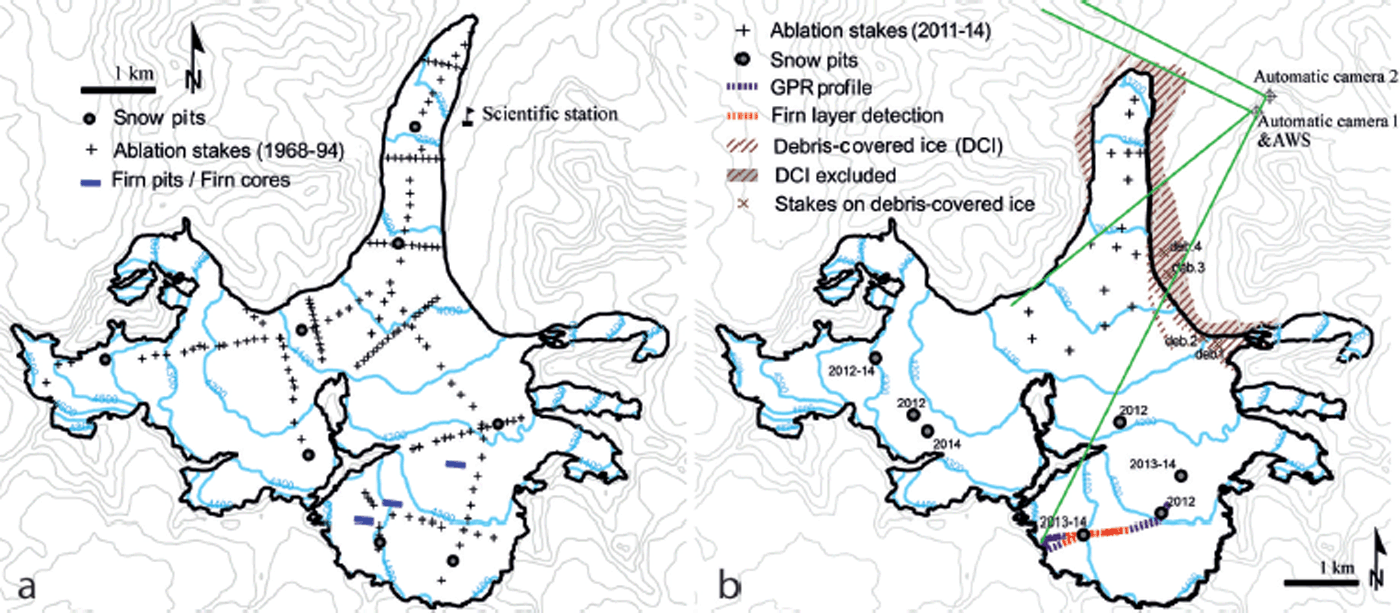
Fig. 3. (a) Stake and snow-pit network on Abramov glacier during 1968–98. The firn-core and firn-pit locations measured in the early 1970s are also indicated. (b) Stake network in 2011 and snow pits measured in the following years. The locations of terrestrial automatic cameras with their view angle (green), the AWS and the GPR profile collected in 2013 are indicated. The red line corresponds to the locations for which a comparison between long-term glaciological measurements, GPR data and geodetically derived elevation changes is performed.
2.1. Glaciological measurements
In 1967, the Central Asian Hydrometeorological Research Institute (SANIGMI) built a glaciological research station near the glacier front (Fig. 3a). We used observations of (1) monthly to seasonal mass-balance components (ablation and accumulation), and (2) standard meteorological variables (Table 1). The observations were carried out continuously from 1968 until 1998. The glacier-monitoring programme of that time included glaciological measurements along 13 profiles (with a total of 165 stakes) and nine snow pits. The 165 stakes were used to measure snow depth at the end of the accumulation season (end of May). At the end of the ablation season (September) these stakes were used to determine the cumulative melt in the ablation area as well as the snow depth in the accumulation area. Monthly snow density and snow depth measurements were carried out at eight snow pits which were dug down to the last year’s end-of-summer horizon (Reference PertzigerPertziger, 1996).
Table 1. Summary of the different measurements available for this study. The number of annual (n a), summer (n s) and winter point mass-balance measurements (n w), the number of snow density observations (ρ) and their date are given (mth indicates monthly frequency). The availability of locally measured air temperature (T air) and precipitation (P) (y: available) and the number of Landsat (LS) and terrestrial camera (TC) scenes used for snowline observations is stated
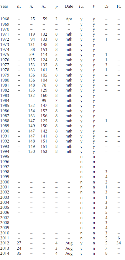
A compilation of these exceptional glaciological data is published in Reference PertzigerPertziger (1996), which is a reference book including a selection of scientific measurements on Abramov glacier acquired by the SANIGMI Glaciological Department. Point values of winter and summer balance are not available to us from 1969 to 1970, and from 1995 onwards (Table∼1). Annual glacier-wide mass-balance data are published from 1968 to 1998 (Reference KamnyanskyKamnyansky, 2001; WGMS, 2005). The data provided by Reference PertzigerPertziger (1996) deliver the base for a consistent re-analysis of the entire series and mass-balance model calibration performed in this study.
Furthermore, repeated measurements of firn density, layer stratigraphy and a temperature profile in three 30 m firn cores from 1972 to 1975 are available (Reference Suslov, Akbarov and YemelyanovSuslov and others, 1980; Reference Glazirin, Kamnyanskii and PerzigerGlazirin and others, 1993). Density, meltwater infiltration and stratigraphy were also determined at two firn pits of up to 17 m depth at elevations of 4250 and 4410 m a.s.l. (Reference Suslov, Akbarov and YemelyanovSuslov and others, 1980) (Fig. 3b).
In 2011 a new network of 16 ablation stakes was set up to represent the previous profile lines and to cover the main features of the surface ablation pattern (Fig. 3b). Since 2012, snow depth and density measurements in three to four snow pits per year have been carried out to determine the annual accumulation from the previous end-of-summer horizon in August (Table 1). The snow pits are located in different accumulation basins. Glaciological measurements have been repeated annually between mid- and late August since 2011. In order to quantify the melt on the strongly debris-covered sections of Abramov glacier, four stakes were installed in 2012 (Fig. 3b).
Ice ablation is converted to water equivalent by assuming a density of 900 kg m−3 (e.g. Reference Beedle, Menounos and WheateBeedle and others, 2014), and through direct density observations in the snow pits for the accumulation zone. An overview of the measurement network is given in Figure 3. The number of available mass-balance data is summarized in Table 1.
2.2. Meteorological data
Standard meteorological variables including daily mean air temperature and precipitation sums were recorded at the glaciological station (3837 m a.s.l.; Fig. 3a), from 1968 to 1994 (Reference PertzigerPertziger, 1996). Solid and liquid precipitation was measured with rain gauges. An AWS was installed in summer 2011 (Reference SchöneSchöne and others, 2013), located at 4100 m a.s.l. and ∼1 km from the former glaciological station (Fig. 3b).
For years with no meteorological in situ measurements (1995–2011) we use data from climate Reanalyses. For precipitation, Reanalysis data were also used from 2012 to 2014. Reanalysis data provide global, continuous and three-dimensional fields of past meteorological variables (Reference Bengtsson and ShuklaBengtsson and Shukla, 1988). Performance is spatially and temporally variable, depending on the number and quality of observations available for the assimilation process. As a result, Reanalyses typically show lower quality at high altitude and in remote regions where observations are sparse (e.g. Reference Trenberth, Stepaniak, Hurrell and FiorinoTrenberth and others, 2001; Reference DuethmannDuethmann and others, 2013). Furthermore, if there are long-term in situ observations available and accessible, these have most probably been used in the Reanalysis assimilation process and thus are not an independent source for evaluating the local Reanalyses. Moreover, the performance during the period with observations is not equal to that in the period without observations. A reduction and assessment of the uncertainty associated with the use of Reanalysis data in remote mountain areas can be achieved by using a set of different Reanalyses instead of only one product.
Here we use the products NCEP/NCAR R1 (US National Centers for Environmental Prediction/US National Center for Atmospheric Research; spatial resolution of 2.5°; Reference KalnayKalnay and others, 1996), ERA-Interim (European Centre for Medium-Range Weather Forecasts re-analysis; spatial resolution ∼0.78°; Reference DeeDee and others, 2011) and MERRA (Modern Era Retrospective-analysis for Research and Applications; spatial resolution of ∼0.55°; Reference RieneckerRienecker and others, 2011), which all provide data since 1979.
2.3. Glacier outlines and digital elevation models
Glacier extent is mapped manually based on Landsat Thematic Mapper (TM)/Enhanced TM Plus (ETM+) and Operational Land Imager (OLI) false-colour composites for each year of the study period as far as an appropriate satellite image is available. For 1972 and for 1975–78, we found satisfactory scenes with a resolution of 79 m, while for 1986–88, 1992, and annually since 1998, scenes with a pixel size of 30 m are available.
Debris-covered glacier ice (∼2 km2) with strongly reduced melt rates (as indicated by ablation measurements) is excluded from the mass-balance calculations. Thin debris cover on the glacier, which is supposed to lower melt rates by <45%, is mapped and included for modelling (Fig. 3b). We adjust the terminus region of the glacier to obtain annual glacier masks for modelling and assume no changes in outline in the accumulation area. Errors related to glacier outlines digitized manually on remote-sensing images depend on atmospheric and topographic corrections, shading, glacier surface characteristics, snow cover and local clouds but mainly on misinterpretation of debris cover (Reference PaulPaul and others, 2013a,Reference Paulb). Uncertainties are expected to be in the range of ±5% of the total glacier area (Reference PaulPaul and others, 2013a), resulting in ±1 km2 in our case.
A digital elevation model (DEM), generated by digitizing contours of a topographic map (1 : 25 000) acquired in 1986 by the Soviet Union-Kyrgyz Office of Geodesy with a cell size of 20 m, and a non-void-filled Shuttle Radar Topography Mission (SRTM) DEM from February 2000 are used. We downscaled the SRTM DEM to a regular 20 m grid using cubic interpolation. The topographic map is based on theodolite measurements collected in 1986 by Reference KuzmichenokKuzmichenok (1990). We compared the DEM from 1986 to the theodolite measurements and found a root-mean-square error (RMSE) of 4 m. To avoid a shift in the two DEMs, we applied a co-registration as proposed by Reference Nuth and KääbNuth and Kääb (2011).
2.4. Terrestrial camera and satellite images
Two terrestrial cameras (Mobotix M25) were installed in August 2011. One camera is located next to the AWS, and the other ∼500 m away at an elevation of 4200 m a.s.l. (Fig. 3b). The digital cameras allow monitoring of the transient snowline on the glacier and take eight oblique photographs per day. Pictures with fresh snowfall are discarded. Due to multiple camera failures and power supply problems, pictures are lacking from the end of the 2012 ablation season to the end of the 2013 ablation season, and again partly for the summer months in 2014. Six camera images from late August to late September 2011, and 34 images from June to mid-August 2012 were used for snowline mapping (Table 1). In addition to the terrestrial photographs, we use orthorectified and georeferenced Landsat TM/ETM+ and OLI scenes to repeatedly observe the snowline throughout the melting season (e.g. Fig. 4). A total of 71 satellite images with suitable conditions are available for 1972–2014 (Table 1). Additional information on historical transient snowline position is given in earlier publications (Reference Suslov, Akbarov and YemelyanovSuslov and others, 1980; Reference Glazirin, Kamnyanskii and PerzigerGlazirin and others, 1993). The snowline on 22/23 August 2012 was mapped in the field with handheld GPS.

Fig. 4. False-colour Landsat images for the 2006 ablation season. The snow depletion pattern is clearly visible. Dark blue areas indicate bare-ice surfaces; light blue areas are snow-covered. The manually delineated snowline is shown in red.
2.5. Ground-penetrating radar
In summer 2013, an 800 MHz GPR survey (MALÅ Geoscience ProEx System) was conducted on the eastern tributary to investigate the firn stratigraphy (Fig. 3b). The antenna was mounted on a sledge that was pulled at a walking speed of ∼1ms−1 taking two measurements s−1. For each measurement, 2048 samples were recorded for a time window of 250 ns. Measurement positions are available from a single-frequency GPS receiver. The GPR profile stretched from the top of the eastern tributary across its accumulation area down to an elevation of 4100 m a.s.l. The entire profile has a length of 2.94 km of which a section of ∼1 km was used for the analysis of the firn layers (red line in Fig. 3b). This section was chosen according to the proximity to former glaciological measurements, spatial continuity, good visibility and the regularity of the detected reflectors.
3. METHODS
This study is structured into three working steps focusing on
(1) the period 1971–94, sustained by detailed seasonal in situ data for annual optimization and calibration of a mass-balance model, (2) the mass-balance reconstruction for the years 1968–70 and 1995–2011, where only limited direct measurements exist, and (3) the analysis of the data collected in 2012–14 from the newly installed monitoring network. All three steps rely on the application of a further developed version of the distributed mass-balance model by Reference Huss, Bauder and FunkHuss and others (2009) in combination with a simplified energy-balance approach to calculate melt as proposed by Reference OerlemansOerlemans (2001). This model is used for steps (1) and (3) as an interpolation tool to obtain mass-balance values for each gridcell at daily temporal resolution based on in situ field data extrapolating them using physical relations. We aim at the best possible representation of glacier-wide mass balance as documented by the direct point measurements and do not focus on detailed physical process understanding. For (1) and (3) the model is calibrated for each year individually with the field measurements. The spatial mass-balance distribution is directly deduced from the in situ measurements, and observed melt and accumulation are related to meteorological input data via tuned parameters. For step (2) the model is driven using the summarized parameters found for the years with measurements. An additional model optimization strategy is adopted using snowline observation on remote-sensing imagery to estimate mass-balance in the best possible way. This recalibration approach is described in more detail in Section 3.5.
3.1. Surface mass-balance model
Snow and ice melt is calculated based on a simplified energy-balance approach after Reference OerlemansOerlemans (2001). The cumulative melt M cum for each gridcell (x, y) of the glacier and each time step (Δt = 1 day) is obtained using
where L m is the latent heat of fusion of ice (334 kJ kg−1). The daily mean surface energy flux Ψd is parameterized as
where Q E is the mean daily potential clear-sky solar radiation and α is the albedo of the snow/ice surface. Τ is the total transmissivity of the atmosphere including cloud cover. Following Reference OerlemansOerlemans (2001) τ is held constant at a value of 0.65 due to a lack of data on cloudiness to constrain this parameter. Furthermore, Reference Machguth, Purves, Oerlemans, Hoelzle and PaulMachguth and others (2008) showed that, compared to other parameters, mass balance is not highly sensitive to τ. T air is the 2m air temperature outside the glacier boundary layer. The term (C 0 + C 1 · T air) describes the sum of the longwave radiation balance and the turbulent sensible heat exchange linearized around the melting point (Reference OerlemansOerlemans, 2001). For simplification, we use a constant value of −50 W m−2 for C 0 and only calibrate C 1. We use different values for the albedo of snow, ice and firn but assume that they are constant over time. The spatial resolution of the model is 20 m. Air temperature is calculated for each gridcell with a constant lapse rate of −4.8°C km−1 (determined from direct measurements after Reference Glazirin, Kamnyanskii and PerzigerGlazirin and others, 1993). A melt reduction of 45% over debris-covered ice (Fig. 3b) is applied after the depletion of the winter snow. This reduction factor has been derived from comparison of observed melt rates over debris and bare-ice surfaces. Q E is calculated for each gridcell and each day of the year, taking into account slope, aspect, topographic shading and a standard atmosphere depending on elevation according to Reference HockHock (1999).
Snow accumulation C at any location (x, y) and time t is calculated based on the sum of solid precipitation:
Solid precipitation is defined as all precipitation that falls below a threshold temperature set to 1.5°C, with a linear transition range of ±1°C (e.g. Reference HockHock, 1999). The amount of solid precipitation at the weather station P ws is corrected with the parameter C prec in order to account for gauge undercatch, a shift of the measurement location and other systematic differences. C prec is calibrated in order to match direct winter point mass-balance measurements as closely as possible. Multiplication with a spatial snow distribution factor D S(x, y) (Reference Tarboton, Chowdhury and JacksonTarboton and others, 1995; Reference Farinotti, Magnusson, Huss and BauderFarinotti and others, 2010) allows the approximation of a plausible distribution of winter accumulation, including topographic effects, wind redistribution and non-altitude-dependent small-scale effects. This dimensionless, spatial accumulation map is derived from inverse-distance interpolation of the point winter balance measurements, normalized over the entire glacier area. D S(x, y) is computed for all years with sufficient measurements (i.e. 1971–94). D S(x, y) for years with no such measurements is taken from years with abundant data, assuming similar spatial accumulation variability from year to year (e.g. Reference Helfricht, Schöber, Schneider, Sailer and KuhnHelfricht and others, 2014).
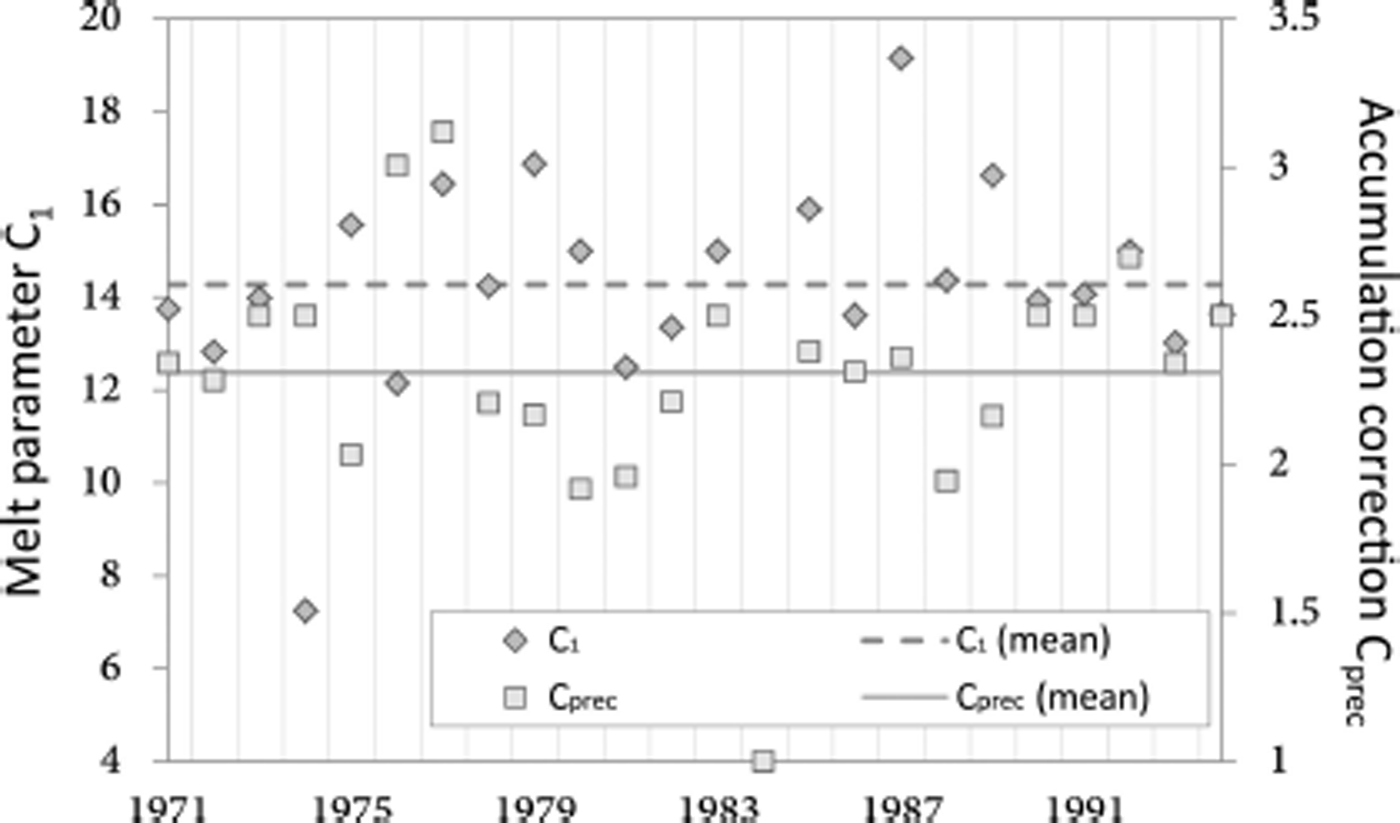
The combined model for accumulation and melt is calibrated to the point measurements for each year individually in a three-step procedure (Fig. 5):
-
1. The dimensionless accumulation pattern D S(x, y) is computed from the winter point balance measurements.
-
2. The winter mass balance is modelled with an initial parameter set. C prec is then adjusted iteratively in order to optimally match the winter snow depth measurements.
-
3. The model is run over the entire balance year using C prec from step 2, and the melt parameter C 1 is iteratively adjusted to match the annual point measurements.

Fig. 5. Model procedure including the automated optimization of the parameters of the distributed mass-balance model (modified after Reference HussHuss, 2010).
The final result is a daily mass-balance series for every glacierized gridcell, which agrees with all available point measurements. For 1968–94 a RMSE of 0.152 m w.e. for the winter point balance and 0.48 m w.e. for the annual point balance is found. The annually optimized parameters from 1971 to 1994 were averaged (Fig. 6). We use this set of parameters to compute the mass balance for the years 1969–70 and 1995–2011, for which no in situ point mass-balance measurements are available.

Fig. 6. Annually calibrated melt and accumulation parameters. Horizontal lines indicate the average of the annually optimized model parameters.
Annual glacier-wide mass balances are given in a fixed-date system (Reference CogleyCogley and others, 2011) and correspond to the hydrological year (1 October–30 September). However, field surveys follow a floating-date system and do not perfectly match the hydrological calendar dates. We use the mass-balance model as a tool to correct the measurement period to the hydrological year. A conventional mass balance (Reference Elsberg, Harrison, Echelmeyer and KrimmelElsberg and others, 2001), i.e. balances are calculated over a changing glacier surface, is presented. This allows direct comparison between glaciological and geodetic methods. Here, only the area is adjusted and surface elevation is updated on an irregular basis. The impact of using the DEM from 1986 instead of that from 2000 on calculated annual mass balances is +0.02 m w.e. a−1, which is not significant at the 5% level. We use the DEM from 1986 for the period 1968–94 and the DEM from 2000 for 1995–2014.
3.2. Internal accumulation and basal ablation
Whereas on temperate glaciers the mass change is dominated by surface components, contributions from the internal and basal mass balance might not be negligible on cold and polythermal high-latitude and high-altitude glaciers (Reference Shumskii and KrausShumskii and Kraus, 1964). In order to estimate the internal–basal mass balance of Abramov glacier, a set of simple models has been developed to quantify the importance of (1) refreezing meltwater in firn layers, and (2) basal melting due to geothermal heat flux and friction.
Our estimate of refreezing is based on calculating a temperature profile in firn and ice using the heat conduction equation (see, e.g., Reference Pfeffer, Meier and IllangasekarePfeffer and others, 1991). The temperature profile is updated in daily time steps driven by surface temperature which, for simplicity, is assumed to equal the air temperature. The one-dimensional model runs separately for each gridcell and is discretized in 0.1 m depth layers. The depth-dependent thermal conductivity is estimated from firn densities as inferred from a simple densification model (Reference Herron and LangwayHerron and Langway, 1980). The model is coupled with the surface mass-balance model that provides the quantity of meltwater for every gridcell and day. The latent heat exchange due to the penetration of the surface meltwater is then calculated and allows determination of the quantity of refrozen water in every layer. To evaluate internal accumulation we are only interested in the refreezing taking place in layers older than 1 year. We assume that the bare ice surface is impermeable. Internal accumulation is thus restricted to the firn zone (Reference Pelto and MillerPelto and Miller, 1990).
The refreezing model is calibrated by adjusting firn temperature at the bottom of the profile at model initialization to match repeated firn temperature measurements made in three firn cores (Fig. 3b) (Reference Glazirin, Kamnyanskii and PerzigerGlazirin and others, 1993). Finally, we compared our results to direct estimates of internal accumulation based on a method described by Reference BazhevBazhev (1973). These measurements on Abramov glacier were acquired in two 12–17 m deep firn pits (Reference Suslov, Akbarov and YemelyanovSuslov and others, 1980). Measurements on Abramov glacier in the early 1970s showed that typically 90–93% of the infiltrated meltwater refreezes in the first four annual layers (Reference Suslov, Akbarov and YemelyanovSuslov and others, 1980). Overall refreezing for the three years ranges between 0.16 and 0.27 m w.e. a−1 at the upper firn pit. The comparison reveals that we overestimate internal accumulation by ∼0.03 m w.e. a−1 at these locations. We estimate the total contribution of the annual internal accumulation to be ∼20% of the total mass balance in the accumulation area, which is in line with findings at Sary-Tor glacier, central Tien Shan, by Reference Dyurgerov, Liu and XieDyurgerov and others (1995).
Our quantification of basal melting is based on simple considerations of the heat balance and the assumption of a temperate glacier bed. We adopt a literature value for the geothermal heat flux (0.05 W m−2; Reference Bagdassarov, Batalev and EgorovaBagdassarov and others, 2011) for the Kyrgyz Tien Shan, and convert it to melt using the latent heat of fusion. Basal friction and strain heating, as two other components of basal–internal mass loss, are approximated by complete dissipation of the potential energy released through gravitational glacier flow. Based on typical values of ice thickness, the bedrock slope and flow velocities of Abramov glacier (Reference Glazirin, Kamnyanskii and PerzigerGlazirin and others, 1993), the released energy is estimated and converted to an equivalent melt. The total quantity of basal ablation is estimated as −0.02 m w.e. a−1.
3.3. Adjustment of Reanalysis data
For the missing years of the climate record, we use three different climate Reanalyses (NCEP/NCAR, ERA-Interim, MERRA). For each Reanalysis, the four nearest gridpoints to Abramov glacier are compared to the in situ meteorological data during the period covered by both series. In order to enforce consistency between local station data and Reanalysis products for the periods in which both data are available, we adjusted the Reanalysis data by applying mean monthly additive (multiplicative) biases for air temperature (precipitation). From the so-corrected monthly means we generate daily series by superimposing day-to-day variability observed at the meteorological station from 1968 to 1994. Thereby we chose the variability of a corresponding month randomly from a year between 1968 and 1994. We generate air temperature series for 1995 to 2011 and precipitation series for 1995 to 2014, for when no measurements are available.
3.4. Model validation
Model validation is performed by using observations of the snow-cover depletion pattern on remote imagery. Oblique ground-based photographs are first corrected automatically for lens distortion with the software PTLens (http://epaper-press.com/ptlens/), then georeferenced and orthorectified after Reference CorripioCorripio (2004) in order to associate every pixel of the photograph to the elevation of the DEM (Fig. 7a and b). Georeferenced Landsat TM/ETM+/OLI satellite (false-colour composites) and terrestrial camera images provide binary information regarding the surface type (snow/ice) of a pixel located on the glacier. The snow-covered area is manually digitized by visual separation of bare ice and snow (Reference Hulth, Rolstad Denby and HockHulth and others, 2013; Reference HussHuss and others, 2013). Manual detection allows integration of the knowledge of the observer on snow-cover depletion patterns and is assumed to be less error-prone than an automatic classification (Reference HussHuss and others, 2013).

Fig. 7. (a) Oblique terrestrial image, (b) georeferenced terrestrial camera image and (c) a Landsat image of Abramov glacier. In (a) and (b) the observed snowline is indicated in red, and the snow-free area is shown in purple. The image refers to 7 September 2011. In (c) the snowlines detected on a satellite image (red) and on a georeferenced photograph (yellow) for 7 September 2011 are depicted.
The transient snowline separates bare-ice from snow-covered areas during the ablation season (Reference PeltoPelto, 2011). At the end of the balance year and under the precondition that no superimposed ice is present, the mean snowline altitude (SLA) approximately corresponds to the equilibrium-line altitude (ELA) (Reference LaChapelleLaChapelle, 1962; Reference LliboutryLliboutry, 1965). The snow-covered area fraction (SCAF) at a given point in time is the fraction of the total glacier surface that is covered by seasonal snow at that time. This measure is similar to the accumulation area ratio, describing the same quantity at the end of the balance year in a stratigraphic system (Reference Mernild, Lipscomb, Bahr, Radić and ZempMernild and others, 2013). We detect the SLA and SCAF on remotely sensed imagery (Landsat, terrestrial camera) and use them as a proxy for sub-seasonal mass-balance by comparing them to the corresponding modelled quantities (Reference PeltoPelto, 2011; Reference HussHuss and others, 2013). The acquisition date on a few satellite images agrees with the terrestrial photographs. This allows comparing the snowline delineation using two different image sources (Fig. 7c). The match is satisfying, with a slight tendency to a higher mean SLA detected on Landsat images (vertical offset <10 m). The accuracy of the observed SLA and SCAF depends on the uncertainties in (1) the snowline delineation, (2) the DEM and (3) the georeferencing of the images (Reference HussHuss and others, 2013). We estimate the uncertainties of the snowline as <100 m (5 pixels) in a horizontal plane on the remote-sensing images. From this, a maximal vertical error of 30 m results when using the mean slope of the glacier. This estimate agrees with Reference Wu, He, Guo and ChenWu and others (2014). For the SCAF we assume an uncertainty of ±3% based on the same analysis.
3.5. Second-order model parameter adjustment
For the period 1995–2011, for which neither direct meteorological data nor glaciological measurements are available (Table 1), the calibrated mass-balance model is driven with the three different climate Reanalysis data series and is validated with SLA and SCAF observations as described in Section 3.4.
The information provided by snowline observations based on the multiple Landsat scenes (Table 1) is used to recalibrate the model parameters for each year from 1998 to 2011. With this second-order adjustment we aim at a better match between modelled and observed SLA and SCAF and thus a better representation of that year’s mass balance.
3.6. Extracting firn layer water equivalents
A series of processing steps was applied to the GPR data as described in Sold and others (Reference Sold, Huss, Hoelzle, Andereggen, Joerg and Zemp2013, Reference Sold, Huss, Eichler, Schwikowski and Hoelzle2015), involving frequency bandpass filtering to reduce noise; background removal; the application of a gain function to compensate for signal attenuation with depth; and spatial interpolation to a 0.5 m equidistant spacing of traces to account for variations in the walking speed. Migration was found not to improve the data quality and was not applied. The vertical resolution of the GPR signal depends on the signal bandwidth. It is typically estimated as half the wavelength (Reference JolJol, 2009), corresponding to <0.13 m for firn densities greater than 530 kg m−3.
The processed GPR data revealed a maximum of 13 pronounced internal reflection horizons (IRHs) reaching up to ∼18 m depth (Fig. 8). For the analyses of the firn layers we only used the sections of the profile with a minimum of seven continuous layers and homogeneous IRHs, which are located in the vicinity of long-term glaciological measurements. A total length of ∼1 km satisfies these criteria (red line in Fig. 3b). The IRHs were interpreted as high-density or ice layers that formed at previous summer surfaces. The correspondence of density peaks to summer surfaces is supported by the core-based firn stratigraphy by Reference Glazirin, Kamnyanskii and PerzigerGlazirin and others (1993) which covers the period 1935–74. As discussed below, we assumed that all detected layers are of annual origin and that their chronology is given by counting from top to bottom.

Fig. 8. A selected section of the processed GPR profile (Fig. 3b) acquired in the accumulation area of Abramov glacier on 17 August 2013. IRHs used to extract accumulation rates are indicated. IRHs were detected to a maximum depth of ∼18 m. Not all layers are continuous over the entire profile, in particular layers at greater depth.
In order to extract accumulation rates from IRHs in the GPR profile acquired in summer 2013, an estimate of the firn density is required to obtain the radio-wave velocity and layer water equivalents. We apply a simple transient model for firn compaction (Reference Herron and LangwayHerron and Langway, 1980; Reference ReehReeh, 2008) where the change in density is linearly related to the pressure from overlying firn layers. The model is applied in a step-by-step procedure (Reference Sold, Huss, Eichler, Schwikowski and HoelzleSold and others, 2015): For the uppermost layer, representing the accumulation of 2013, density is set to 530 kg m−3, based on the two density field measurements taken on the eastern tributary next to the GPR profile (Fig. 8). Using an empirical relation of the dielectric permittivity with snow density (Reference Frolov and MacheretFrolov and Macheret, 1999) we obtain the signal velocity in the snow. Thereby, we assume that the effect of liquid water in the snowpack on the signal velocity is negligible. This is supported by the good agreement found between the depth of the snow density pit (2.40 m) and the GPR-derived snow depth (2.44 m) at the same location. The signal velocity and the snow density is then provided for every GPR measurement location, leading to an estimate for the thickness and water equivalent of this layer and, thus, for its weight on the underlying layers at each GPR measurement location. Then the firn compaction model can be used to obtain the density of the second firn layer. By stepping through the firn layers from top to bottom an estimate for the water equivalent of each layer is derived.
The model is calibrated with repeated density observations in two firn pits in the early 1970s published by Reference Suslov, Akbarov and YemelyanovSuslov and others (1980) corresponding to the location of meltwater infiltration measurements (see Section 3.2). Calibrated parameters are in line with Reference HussHuss (2013) who found a similar densification rate when fitting the model to a set of density profiles from 19 firn cores for temperate and polythermal mountain glaciers and ice caps around the globe.
The GPR-derived accumulation rates are sensitive to potential perturbations in the chronology of IRHs in the radar profiles. As no reference data, such as from firn cores, are available to corroborate the dating of IRHs, this is a major drawback to the approach presented here. As stated above, however, the firn stratigraphy record by Reference Glazirin, Kamnyanskii and PerzigerGlazirin and others (1993) for the period 1935–74 supports the correspondence of high-density layers to summer surfaces. On the other hand, some annual layers were not present in this record. This is supported by past in situ measurements which indicate that the ELA sporadically rose above the elevation of the radar profile. As a consequence, we assume that we potentially missed individual accumulation layers but that we did not detect reflectors other than from summer surfaces. Hence, the presented accumulation rates obtained from IRH travel times provide an upper limit estimate for the local accumulation rates and the results are interpreted accordingly.
3.7. Uncertainty analysis
The overall uncertainty in the calculated glacier-wide mass balance was assessed through a cross-validation experiment for the periods with available point data (1971–94, and 2012–14). We randomly selected 75% of the point measurements for each seasonal survey and recalibrated our model to those data. The remaining 25% of the measurements were used as a validation subset. This procedure was repeated ten times with different random subsets. Model uncertainty was estimated by computing the RMSE of the difference between modelled and measured mass balance for the points in the validation subset. Under the assumption that (a) the model performance is identical for every point location on the glacier and (b) the uncertainties of individual years are independent of each other, the calculated mean RMSE for both the winter and annual mass balance is interpreted as the uncertainty in the corresponding glacier-wide mass balance. We found mean uncertainties in winter and annual balance for the above-mentioned periods of ±0.21 and ±0.47 m w.e. a−1, respectively.
The uncertainties for the periods 1969–70 and 1995–2011, i.e. the years for which no direct field measurements are available, primarily depend on (1) the chosen model parameters and (2) the quality of the meteorological input data. In order to quantify the uncertainties for these periods, we run the mass-balance model for 1971–94 (the period with direct glaciological measurements) with average parameters, i.e. those used for 1995–2011. Based on comparison with the annually optimised glacier-wide mass-balance we derive a mean RMSE of 0.30 m w.e. a−1.
To estimate the uncertainty related to the meteorological input data, we drove the mass-balance model with the three different climate Reanalysis products. The differences between the modelled balances and the final glacier-wide balance obtained after the second-order parameter adjustment (i.e. our best estimate) are calculated for eachyear individually. The RMSE of the differences was 0.43 m w.e. a−1, which was interpreted as the error introduced by the uncertainty of meteorological data for the period with no direct measurements. Combining the above uncertainties on quadrature, i.e. assuming independence between individual error sources, the total uncertainty for yearly values during the period with no glaciological data available is ±0.54 m w.e. a−1. Note that when calculating the average over a period of n years (e.g. Table 4), this value is reduced by a factor
![]() , as given by the rule of Gaussian error propagation.
, as given by the rule of Gaussian error propagation.
4. Results
Availability of in situ mass-balance data between 1971 and 1994 is optimal (Table 1). Our re-analysed surface mass-balances are compared to published series that are based on traditional evaluation techniques such as the profile- and contour-line method (Reference Kaser, Fountain and JanssonKaser and others, 2003; Table 2).
Table 2. Summary of re-analysed mean annual surface mass balance from 1971–94 compared with literature-based values
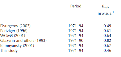
We found an average annual surface mass balance of −0.46 ±0.06 m w.e. a−1 (1971–94) (Fig. 9) which is less negative than stated in most of the earlier literature but corresponds to the recalculated series by Reference DyurgerovDyurgerov (2002). The major discrepancies with Reference PertzigerPertziger (1996), Reference KamnyanskyKamnyansky (2001) and WGMS (2005) are explained by data gaps (1984) and years with poor data coverage (1974–76). By using the profile- or contour-line method, large errors in the calculated mass balance propagate with increasing elevation, leading to considerably too negative mass balance. A different glacier surface hypsometry, mainly around the elevation of the ELA, also explains some of the disagreement between the studies. Furthermore, a misinterpretation of the area–altitude distribution causing a shift in the elevation bins has been discovered in some publications. In the past, ablation stakes were grouped together and a mean elevation was attributed for mass-balance calculation. More recent publications use regular 100 m elevation bins for the same data, which leads to a vertical shift of the hypsometry of up to 100 m.

Fig. 9. (a) Mean annual air temperature (MAAT) and (b) annual precipitation from direct observations and Reanalysis data. (c) Re-analysed annual mass balance (bars) and cumulative balance (lines) for Abramov glacier from 1968 to 2014. Dark grey bars indicate the years sustained by glaciological measurements, and light grey bars show years with no point measurements. After 1995, cumulative mass balances generated from different climate Reanalyses are shown (dashed lines). The thick black line indicates the optimal series found by comparison with SLA and SCAF observations by remote imagery.
From 1971 to 1994, the observed transient snowlines on Landsat images are well approximated by the model (RMSESLA = 45 m; RMSESCAF = 6%), and the results qualitatively match snowline observations from the literature (Reference Suslov, Akbarov and YemelyanovSuslov and others, 1980; Reference Glazirin, Kamnyanskii and PerzigerGlazirin and others, 1993). The amount of available remote-sensing images with good quality is unfortunately limited for this period, hampering a sound validation.
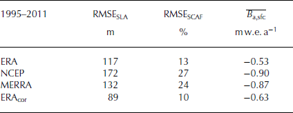
The three Reanalysis datasets used result in a range of mass balance for 1995–2011 (Fig. 9). From our validation using SLA and SCAF observed on Landsat scenes and comparison of overlapping periods with both in situ meteorological and Reanalysis data, we conclude that ERA-Interim yields the most plausible results (Table 3). The applied second-order adjustment on the mass-balance model driven with ERA-Interim data from 1995 to 2011 noticeably reduces the RMSE of SLA (90 m) and SCAF (10%) (Table 3). However, years with only a small number of remote-sensing images during the ablation season such as 2001 and 2003 (Table 1) are problematic for the annual adjustment. For the period 1995–2011, the glacier-wide average surface mass balance for the annually corrected series decreases from −0.53 m w.e. a−1 to −0.63 m w.e. a−1 (Table 3) and becomes less negative than the uncorrected values for the years 1995–2000 and more negative for 2000–11 (Fig. 10).

Fig. 10. Comparison of the calculated annual mass balance 1995–2011 before (uncorrected) and after (corrected) the second-order adjustment of the model parameters to match annual SLA and SCAF observations. The error bars indicate uncertainties calculated as described in Section 3.7.
Table 3. Comparison of mean annual balance
![]() and the RMSE for SLA and SCAF when using different Reanalysis products. ERAcor indicates the result obtained for ERA-Interim data and readjusted model parameters to match annually the SLA and SCAF
and the RMSE for SLA and SCAF when using different Reanalysis products. ERAcor indicates the result obtained for ERA-Interim data and readjusted model parameters to match annually the SLA and SCAF
The balance years 2011/12 to 2013/14 show considerable mass loss (Fig. 9). Observed SLAs and SCAFs from 2012 to 2014 are reproduced by the model within a range of ±41 m and ±3.4%, respectively. With the higher frequency of high-quality images the confidence of the validation increases (Fig. 11).

Fig. 11. Modelled transient snowline altitude during the 2012 ablation season (from June to the beginning of September) and observations on terrestrial photographs (circles), Landsat images (diamonds) and in situ GPS measurements (triangle).
From 1968 to 2014 (Fig. 9), the glacier-wide mass balance is predominantly negative. We found a mean annual surface mass balance of −0.51 ± 0.10 m w.e. a−1 (Table 4) and a basal–internal balance of +0.07 m w.e. a−1.
Table 4. Seasonal mass balance of Abramov glacier from 1968 to 2014 with B w,sfc the winter mass balance (1 October–31 May), B a,sfc the annual surface balance over the hydrological year, B i–b the internal–basal mass balance and ΔM the total annual glacier mass balance
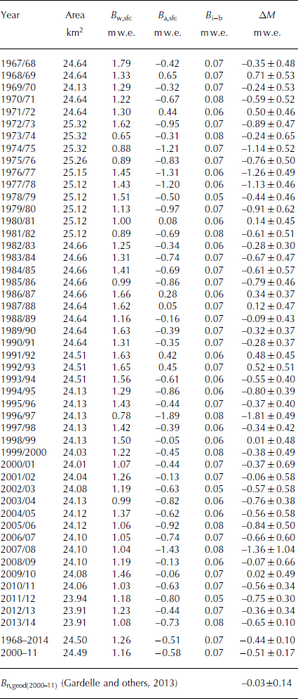
Both the components of internal and basal balance are one to two orders of magnitude smaller than the surface mass balance but still need to be taken into account for long-term studies of glacier mass change and the comparison to geodetic mass balance.
5. Discussion
5.1. Climate sensitivity
A prerequisite for the application of empirical positive degree-day models for the calculation of snow and ice melt is the correlation between air temperature and the melt rate (see Reference OhmuraOhmura, 2001, for the physical background). For Abramov glacier, we tested the relation between air temperature and melt by comparing the sum of cumulative positive degree-days (CPDDs) over the summer season to the observed average summer balance at all ablation stakes from 1968 to 1994. For this year-to-year comparison, we found the squared correlation coefficient r 2 = 0.67. The correlation is similar to that for glaciers in the European Alps and Scandinavia (Reference Ohmura and BauderOhmura and others, 2007; Reference Sicart, Hock and SixSicart and others, 2008). Additionally, we compared the summer balance of each ablation stake individually to the annual CPDDs calculated for the corresponding location. This comparison, which excludes effects of elevation, also indicates a satisfying correlation, the average correlation coefficient being r 2 = 0.57, with 80% of the data having an r 2 between 0.35 and 0.78.
Reference OerlemansOerlemans (2001) assessed the sensitivity of Abramov glacier to changes in temperature and precipitation by using a calibrated energy-balance model of intermediate complexity. According to that study, the mass balance of Abramov glacier is less sensitive to changing climatological conditions than that of glaciers located in more maritime climates such as Nigardsbreen, Norway, or Franz Joseph Glacier, New Zealand, and is more sensitive than that of continental glaciers such as White Glacier, Canadian Arctic. The sensitivity of Abramov glacier to temperature changes during the summer months is pronounced; sensitivity to precipitation, on the other hand, is relatively low and constant throughout the year (Reference OerlemansOerlemans, 2001). Reference RasmussenRasmussen (2013) used Reanalysis data (NCEP/NCAR products) to investigate glacier sensitivity to air temperature and precipitation on selected glaciers in High Asia. For Abramov glacier a relatively high temperature sensitivity of δB = −0.47 m w.e. °C−1, and a high correlation between the Reanalysis temperature and interannual variations of glacier-wide summer surface mass balance was found.
5.2. Mass-balance variations
The evolution of the mass-balance distribution with elevation and time (Fig. 12) reveals a weak tendency towards more accumulation at higher elevation but also more ablation during the past few decades. This indicates a shift in the mass turnover of Abramov glacier. A similar change in the accumulation and ablation pattern is indicated for the entire Pamir region by Reference Glazirin, Braun and ShchetinnikovGlazirin and others (2002) and Khromova and others (Reference Khromova, Osipova, Tsvetkov, Dyurgerov and Barry2006, Reference Khromova, Nosenko, Kutuzov, Muraviev and Chernova2014). Reference Kure, Jang, Ohara, Kavvas and ChenKure and others (2013) project an increase in monthly mean precipitation from November through April but simultaneously a reduction in snowfall from February through October for the next 100 years. The reduced snowfall in spring and autumn can be linked to a rise in air temperature. Reference Lutz, Immerzeel, Gobiet, Pellicciotti and BierkensLutz and others (2013) and Reference WangWang and others (2014) support this finding with similar results for the whole of Central Asia. Studies from the nearby Karakoram region show that increased winter snowfall can compensate for increased melt rates in summer (Reference Gardelle, Berthier, Arnaud and KääbGardelle and others, 2013; Reference Mandal, Ramanathan and AngchukMandal and others, 2014; Reference Kääb, Treichler, Nuth and BerthierKääb and others, 2015) for high-elevation glaciers that consequently exhibit a reduced sensitivity to air temperature changes.

Fig. 12. Elevation dependence of the mass balance averaged for the indicated periods (lines), and surface hypsometry (as of 2013) of Abramov glacier (bars).
5.3. Comparison of modelled point balance and GPR data
From 2001 to 2013 the GPR observations indicate substantially higher accumulation rates than the modelled point balance (mean difference of 0.500 ± 0.36 m w.e. a−1). As stated above, the GPR-derived layer water equivalents were considered as upper limit estimates of the annual mass balance because one or several previous summer surfaces might be absent in the GPR data. A direct comparison with observations is impeded by the lack of glaciological mass-balance measurements in that period. To estimate the contribution of the mass-balance model to the encountered difference, we compared the modelled point balance based on the averaged parameter set (i.e. parameters used for 1995–2011), and thus independent of the stake measurements, to the in situ measurements available for a location on the radar profile (red dot in Fig. 3b). A difference of +0.36 ±0.31 m w.e. a−1 was found. This explains two-thirds of the disagreement between the modelled and the GPR-based point balance. We conclude that the higher accumulation rates derived from GPR do not conflict with the re-analysed mass-balance time series, but can be attributed to local effects at the location for which water equivalents were extracted and the uncertainties in the layer chronology. Because the latter poses a substantial drawback to the GPR-based derivation of annual accumulation, the data were not used to constrain the mass-balance model.
5.4. Comparison of modelled and geodetic mass- balance 2000–11
Our results on the mass-balance evolution between 1971 and 1994 are well constrained by the high number of seasonal in situ observations. The inferred mass balance between 1995 and 2011 is, however, less certain since it relies on modelling and sparse and temporally inhomogeneous information on snow-covered area. Due to the low quality of the available DEMs, it was not possible to compute a geodetic mass balance from 1986 (topographic map) to 2000 (SRTM DEM). However, Reference Gardelle, Berthier, Arnaud and KääbGardelle and others (2013) provide an independent estimate for the mass change of Abramov glacier. By differencing the SRTM DEM of February 2000 and a SPOT5 (Satellite Pour l’Observation de la Terre) stereo image from November 2011, the authors estimate an average mass balance of −0.03±0.14 m w.e. a−1, thus indicating a balanced mass budget. Reference Gardelle, Berthier, Arnaud and KääbGardelle and others (2013) report significant positive elevation changes in the accumulation area compensated by surface lowering below the ELA. This is in contrast to our results indicating a total balance of −0.51±0.17 m w.e. a−1 from 2000 to 2011.
To verify the plausibility of surface elevation changes derived by Reference Gardelle, Berthier, Arnaud and KääbGardelle and others (2013) we combine the long-term series of accumulation available for several locations in the vicinity of the GPR profile (Fig. 3a; Table 1) with the recent accumulation rates inferred from GPR. This is achieved by applying simple considerations of glacier dynamics. The elevation change Δh at a given point in the accumulation area is determined by the local long-term mean of point mass balance Δb, the change in mass balance Δb relative to a reference period, and the vertical ice flow velocity v z as
where ρ firn is the firn density and ρ w the water density. Δt is the time period considered. If we suppose a steady state over the reference period (Δh = 0), the local mass change b is balanced by the vertical velocity, resulting in an invariant glacier surface (Reference Cuffey and PatersonCuffey and Paterson, 2010). For any time interval following the reference period we can thus simplify Eqn (4) into
For our case we use Δt = 12 years (2000–11) and estimate Δb from the change in local mass balance that has occurred over the past decade (2001–14) compared to the reference period 1968–94. ρ firn is inferred from a firn densification model (Reference Herron and LangwayHerron and Langway, 1980).
For all locations on the GPR profile (Fig. 3b) for which more than seven continuous IRHs have been detected, the dataset by Reference Gardelle, Berthier, Arnaud and KääbGardelle and others (2013) indicates a mean surface elevation change of +5.3 ± 4.7 m. Such positive elevation change in the accumulation area over only one decade is likely to result in strong effects on the glacier outlines in the upper reaches of Abramov glacier. However, no evidence for such behaviour was found in the repeated Landsat images. We calculated the expected elevation change on the profile based on the GPR data and Eqn (5). On average we find Δh = +0.6 ± 0.7 m for the period 2000–11 assuming a steady state of the glacier prior to 1994. Most probably Abramov glacier was already out of balance before then. Hence, the actual Δh would even be somewhat smaller. Given that a similar difference applies to the entire accumulation area, the geodetic mass balance according to Reference Gardelle, Berthier, Arnaud and KääbGardelle and others (2013) would be overestimated substantially. Unfortunately, GPR measurements are limited to a small part of the glacier, but comparison at different locations with long-term in situ measurements in the accumulation area indicates a similar trend.
The geodetic mass-balance calculation might be affected by an underestimation of the C-band penetration over snow and firn previously documented for the SRTM DEM (Reference Rignot, Echelmeyer and KrabillRignot and others, 2001; Reference Gardelle, Berthier and ArnaudGardelle and others, 2012; Reference PaulPaul and others, 2013b). This would be consistent with an over-estimation of positive surface elevation changes in the firn area between 2000 (SRTM DEM) and 2011 (SPOT5). Region-wide mass-balance estimates derived from the Ice, Cloud and land Elevation Satellite (ICESat) for 2003 to 2008 were recently published by Reference Kääb, Treichler, Nuth and BerthierKääb and others (2015). They mentioned a highly variable C-band penetration depth in snow and firn, especially for the Pamir. Reference Kääb, Treichler, Nuth and BerthierKääb and others (2015) estimate the C-band penetration depth of 5–6 m, instead of 1.8 m as used by Reference Gardelle, Berthier, Arnaud and KääbGardelle and others (2013). If we adjust the elevation change reported by Reference Gardelle, Berthier, Arnaud and KääbGardelle and others (2013) accordingly, their estimate is reduced to a mean of +1.1 to −2.1 m at the locations described above. This is close to our independent assessment. If we recalculate the geodetic mass balance from February 2000 to November 2011 for Abramov with a C-band penetration depth of 5–6 m instead of 1.8 m, a glacier-wide mass balance of about −0.25 m w.e. a−1 is found. This value lies within the uncertainties of our reconstructed time series. Comparing theodolite measurements from 1986 and the SRTM DEM from 2000, we find an elevation change of +3.7 to +4.7 m. Using the direct measurements and modelling, the inferred elevation change is +4.2 ± 1.1 m. Again the good agreement underlines the performance of the mass-balance model, also for a period without direct measurements.
A mass balance of −0.48 ± 0.14 m w.e. a−1 is reported for the Pamir from 2003 to 2008 by Reference Kääb, Treichler, Nuth and BerthierKääb and others (2015). Our model-based reconstruction of mass balance in the first decade of the 21st century allows us to assess the temporal dynamics of the mass change of Abramov glacier indicating −0.79 ± 0.25 m w.e. a−1 for the same period. According to our assessment, Abramov glacier thus shows a more negative balance than the mean region-wide mass balance found for the Pamir.
6. Conclusions
For the Central Asian countries little is known regarding seasonal glacier mass balance over the past two decades. A re-evaluation of other monitoring programmes on various glaciers during the 1970s and 1980s is urgently needed. Such long-term mass-balance data are an important data basis for future evaluations of climate-change impacts in a highly vulnerable region, especially in the context of future runoff estimates. With this study we present a first step towards revealing the long-term seasonal mass-balance changes for a reference glacier in the Pamir Alay by combining various sources of historical and modern data.
We aimed at deriving a persistent seasonal mass-balance series for Abramov glacier from 1968 to 2014. Our approach combines seasonal field measurements with distributed modelling at daily temporal resolution. We show that it is possible to validate modelling results with transient snowline observations from satellite images and that these observations provide valuable information on the mass balance of remote glaciers for time periods without direct measurements. The mass-balance model is used as a tool to interpolate and extrapolate annual or seasonal point data in space and time, allowing the establishment of a continuous mass-balance series. Moreover, it allows the interpretation of interannual accumulation and ablation characteristics, their typical distribution and their changes over time.
From our calculations and earlier publications there is no doubt that Abramov glacier has shown a considerable mass loss from the late 1960s until the end of the 20th century. We found convincing evidence that this trend has been continued at the beginning of the 21st century. We infer a mean annual total mass balance of −0.44 ± 0.10 m w.e. a−1 for 1968–2014 resulting from a surface mass balance of −0.51 ± 0.10 m w.e. a−1 and an internal-basal balance of +0.07 m w.e. a−1.
In our re-evaluation of the mass-balance series, we combine direct measurements, remote observations and modelling following the general monitoring strategy defined by Reference ZempZemp and others (2014). The importance of long-term point balance measurements and their value for model calibration is highlighted. Snowline observations on remote imagery provided essential information to allow model validation when no other data were available. Mass change calculations based on geodetic methods suggested a balanced mass budget since 2000 (Reference Gardelle, Berthier, Arnaud and KääbGardelle and others, 2013), contradicting our results. The disagreement can probably be explained by an underestimation of the C-band penetration depth in the SRTM DEM leading to too positive mass-balances. This interpretation is supported by the results of Reference Kääb, Treichler, Nuth and BerthierKääb and others (2015) and our ground-based GPR measurements on Abramov glacier. Because the latter are prone to uncertainties in the layer chronology, the results are not used to reconstruct mass balances and were interpreted according to its limitations. Altogether, we find a low plausibility for equilibrium conditions over the past 15 years. Instead, we suggest that the glacier’s sensitivity to increased summer air temperature is decisive for the strong mass loss assessed for the past decade.
Acknowledgements
The project was only possible due to the support of the Federal Office of Meteorology and Climatology MeteoSwiss through the project Capacity Building and Twinning for Climate Observing Systems (CATCOS) Phase 1 & 2, contract Nos. 7F – 08114.1, 7F – 08114.02.01, between the Swiss Agency for Development and Cooperation (SDC) and MeteoSwiss. This study is supported by the Swiss National Science Foundation (SNSF), grant 200021 155903. Additional support by the German Federal Foreign Office in the frame of the CAWa project (http://www.cawa-project.net) is equally acknowledged. We thank J. Gardelle and E. Berthier for providing the elevation change data of Abramov glacier 2000–11. J. Corripio is acknowledged for the software to georeference oblique photographs. We additionally thank H. Machguth, W. Hagg, A. Gafurov, M. Kronenberg, J. Schmale, D. Sciboz and everyone else that contributed to the fieldwork. We also thank all scientists of the glaciological expedition of the Central Asian Research Hydrometeorological Institute, who carried out the extensive measurements at Abramov glacier in the past. We are also grateful to the Central Asian Institute for Applied Geosciences for their collaboration, especially to B. Moldobekov for his continuous support. Detailed comments by two anonymous reviewers were helpful in finalizing the manuscript.