


Introduction
Food safety is a critical public health concern for consumers and producers (Bellemare and Nguyen Reference Bellemare and Nguyen2018; Bar and Zheng Reference Bar and Zheng2019; Ollinger and Bovay Reference Ollinger and Bovay2020). Despite the economic significance of foodborne diseases and reoccurring illnesses from the consumption of fresh fruits and vegetables, there is a lack of studies on the economic efficiency of ex-ante prevention of food contamination in the fresh produce sector. Nevertheless, in response to numerous foodborne disease outbreaks, the Food Safety Modernization Act (FSMA) was enacted in 2011 to improve food safety and prevent foodborne illnesses, particularly in fresh fruits and vegetables.Footnote 1 Pursuant to FSMA, the Food and Drug Administration (FDA 2014) proposed preventative standards for growing, harvesting, packing, and storage of fresh produce intended for human consumption without processing. According to the FDA, irrigation carries a significant risk of introducing pathogens to the fresh produce supply. Therefore, regulating irrigation water quality is prioritized for foodborne disease prevention (FDA 2012a). The FDA rules require periodic testing of irrigation water and restrict the use of water that exceeds the maximum allowable number of colony-forming units (CFU) of Generic E. coli as an indicator microorganism.Footnote 2
According to the FDA’s FSMA regulation, if a) the statistical threshold value (STV) of E. coli exceeds 410 or b) the moving geometric mean (GM) exceeds 126 CFU per 100 ml of water from any five consecutive irrigation surface water samples or one groundwater sample, then irrigation from the contaminated sources should cease unless water is treated, or harvest should be delayed allowing for microbial die-off (FDA 2014). Growers can delay harvest for up to four days to allow for the die-off of pathogens. The produce that is out of compliance based on half-log reduction of E. coli CFUs after four days must be discarded.
FSMA rules overlap with the Leafy-Greens Marketing Agreement (LGMA) program, adopted in 2007 in response to the 2006 E. coli outbreak linked to spinach. Like FSMA, LGMA aims to protect public health by decreasing foodborne illnesses from leafy greens. The food safety practices in LGMA include environmental assessments, water testing and recordkeeping, soil amendments, worker practices, and field sanitation. LGMA includes shippers and sellers in California and Arizona, who deliver roughly 90% of leafy greens in the U.S. (California Leafy-Greens Marketing Agreements 2022). LGMA irrigation water quality standard is based on a rolling geometric mean of Generic E. coli from five samples. However, if less than five samples are taken before irrigation, the maximum acceptance criteria depend on the number of samples. If only one sample has been collected, Generic E. coli must be less than or equal to 126 CFU/100 ml. If the acceptance criterion is exceeded, two samples must be taken, and a geometric mean should be below 126 CFU/100 ml.
Although FSMA and LGMA have similar testing and microbial water quality requirements, there are also some differences. FSMA standard allows more choices as remedial action relative to LGMA. The remedial actions under FSMA include treating contaminated water, delaying harvest, or extending the period between harvest and storage to allow for microbial die-off. The LGMA requires treating irrigation water to continue production. LGMA requires monthly testing, while FSMA requires a minimum of five (one) samples for untreated surface (ground) irrigation water. Finally, LGMA requires testing water that is either directly or indirectly applied to the produce, while FSMA requires testing only directly applied water (Calvin et al. Reference Calvin, Jensen, Klonsky and Cook2017).
Several studies have examined the FSMA rule. Using an equilibrium-displacement model, Ferrier et al. (Reference Ferrier, Zhen and Bovay2018) estimate that FSMA increases consumer fruit and vegetable prices by 0.49% and 0.14%, respectively. Also, FSMA decreases vegetable and fruit producers’ welfare by 0.59% and 0.86%, respectively. Bovay and Sumner (Reference Bovay and Sumner2017) also use an equilibrium-displacement model to show that wholesale tomato prices increase by up to 2.4% if demand for safer produce rises relative to the scenario with more foodborne outbreaks and no FSMA. Bovay (Reference Bovay2017) uses GAP (Good Agricultural Practices) standards to estimate the likely effects of FSMA on demand for tomatoes from Florida and California and finds that GAPs do not increase demand for fresh tomatoes. Hence, FSMA is not likely to increase demand for fresh produce, which implies reduced farmer profits because a price increase does not offset FSMA regulation costs. In addition, prior studies also showed that, due to scale economies, small farms are disproportionately burdened by FSMA costs (Lichtenberg and Page Reference Lichtenberg and Page2016; Bovay and Sumner Reference Bovay and Sumner2017; Adalja and Lichtenberg Reference Adalja and Lichtenberg2018; Bovay et al. Reference Bovay, Ferrier and Zhen2018).
Our objective is to evaluate the economic merits of the FSMA irrigation water quality regulation as an ex-ante control strategy for foodborne disease in the lettuce market. A theoretical model is developed as a framework for the analysis. Conditions for optimal microbial water quality regulatory stringency are derived as a function of water scarcity, regulation costs, illness severity, and illness prevention efforts of distributors and consumers. Next, the optimality conditions are examined empirically using lettuce as a case study. The FDA rule is examined relative to the existing LGMA guidelines.
The empirical model integrates a dose–response formulation (Lichtenberg Reference Lichtenberg2010; Pang et al. Reference Pang, Lambertini, Buchanan, Schaffner and Pradhan2017) in a stochastic two-stage partial equilibrium framework (Dantzig Reference Dantzig1955; Lambert et al. Reference Lambert, McCarl, He, Kaylen, Rosenthal, Chang and Nayda1995) with recourse. In such models, stage one decisions are made before the stochastic state of nature is revealed. Stage two activities take place after the stochastic state of nature is revealed and are conditional on the decisions made in stage one. In the first stage, before the stochastic irrigation water quality is revealed, farmers make planting and irrigation decisions for the upcoming growing season. In the second stage, water treatment and harvest activities are subject to the FSMA guidelines on the acceptable microbial quality of irrigation water and harvest delay.
The objective function maximizes consumer and producer surplus minus illness costs and costs of standard implementation. This approach extends the FDA (FDA 2014) cost/benefit (CBA) analysis by explicitly accounting for producer and consumer surplus changes. The constraints include demand and supply balance, land use restrictions, stochastic water quality equations, yield and irrigation relationships, harvest, water treatment, storage delay constraints reflecting STV and GM standards, and illness dose–response specifications.
We use lettuce as a case study for several reasons. First, all lettuce is consumed fresh without processing. As such, lettuce is one of the primary targets of FSMA regulation. Second, lettuce is highly perishable. Hence, delay in harvest as a response strategy mandated by FSMA can have significant implications for supply and profitability. Third, several recent severe foodborne disease outbreaks have been traced to contaminated lettuce. For example, according to the Centers for Disease Control and Prevention (CDC), in June 2018, an outbreak of E. coli was traced to romaine lettuce irrigated with contaminated water that affected 210 people in at least 36 states with 96 hospitalizations and 5 deaths (CDC 2018). In January 2019, another E. coli outbreak was linked to romaine lettuce with 167 cases, including 85 hospitalizations (CDC 2020, 2019).
This study contributes to prior literature with an economic evaluation of ex-ante food contamination prevention in the fresh produce sector, focusing on the lettuce market as a case study. We provide a theoretical framework and develop a stochastic partial equilibrium model to examine the stringency of microbial irrigation water quality standard. To our knowledge, this paper is first to examine the food safety-related irrigation water quality standard as proposed by the FDA using an economic framework that includes consumer and producer surplus and a detailed pathogen exposure and dose–response formulations. The results shed new light on the merits of additional regulatory requirements and examine the sensitivity under various parametric assumptions.
Theoritical framework
The regulator’s problem is to maximize social welfare ( $SW$
) in terms of consumer and producer surplus minus the cost of irrigation, expected damages from foodborne illnesses due to water contamination, and cost of implementing water quality standard with respect to irrigation w and water quality standard (
$SW$
) in terms of consumer and producer surplus minus the cost of irrigation, expected damages from foodborne illnesses due to water contamination, and cost of implementing water quality standard with respect to irrigation w and water quality standard ( $\theta $
). The notation is summarized in Table A.1.
$\theta $
). The notation is summarized in Table A.1.
 $$\mathop {\max }\limits_{\theta ,w} SW = \mathop \int \nolimits_0^X P\left( {X\left( w \right),\theta } \right)dX - cw - $$
 $$\left[ {\mathop \int \nolimits_0^\theta S\left( {\mu ,X\left( w \right);\alpha } \right)f\left( \mu \right)d\mu + S\left( {\theta ,X\left( w \right);\alpha } \right)\mathop \int \nolimits_\theta ^z f\left( \mu \right)d\mu } \right] - R\left( {\theta ;\beta } \right)$$
where SW is the social welfare and P(X(w), θ) is the inverse demand for fresh produce X and water quality standard $\left( \theta \right)$
. X(w) is the production function of X in terms of irrigation w.
$\left( \theta \right)$
. X(w) is the production function of X in terms of irrigation w. $S\left( {\mu ,X\left( w \right);\alpha } \right)$
is the monetary value of damages from foodborne illnesses as a function of water quality
$S\left( {\mu ,X\left( w \right);\alpha } \right)$
is the monetary value of damages from foodborne illnesses as a function of water quality $\mu $
, consumption X, and consumer and producers prevention efforts
$\mu $
, consumption X, and consumer and producers prevention efforts $\alpha $
. f(
$\alpha $
. f( $\mu $
) is probability distribution of water quality with low (high) values of
$\mu $
) is probability distribution of water quality with low (high) values of $\mu $
corresponding to better (worse) microbial quality,
$\mu $
corresponding to better (worse) microbial quality, $\mu $
∈{0: z} (Figure A.1, top panel). Water quality is stochastic because farmers are not able to accurately forecast water quality without testing shortly before each irrigation. Therefore, after planting decisions are made, the quality of water used for irrigation during the growing season is random.
$\mu $
∈{0: z} (Figure A.1, top panel). Water quality is stochastic because farmers are not able to accurately forecast water quality without testing shortly before each irrigation. Therefore, after planting decisions are made, the quality of water used for irrigation during the growing season is random. $R\left( {\theta ;\beta } \right)$
is the cost of implementing the water quality standard with
$R\left( {\theta ;\beta } \right)$
is the cost of implementing the water quality standard with $\beta $
as the shift parameter. c is the cost of irrigation water. The term in the square brackets is the expected damage from foodborne illnesses.
$\beta $
as the shift parameter. c is the cost of irrigation water. The term in the square brackets is the expected damage from foodborne illnesses.
The water quality standard $\left( \theta \right)$
truncates the left tail of water quality distribution. If microbial water quality is poorer than the regulatory standard (
$\left( \theta \right)$
truncates the left tail of water quality distribution. If microbial water quality is poorer than the regulatory standard ( $\mu \ge \theta $
), then foodborne illness damages are expressed in terms of
$\mu \ge \theta $
), then foodborne illness damages are expressed in terms of $\theta $
because the regulatory standard truncates microbial contamination of water, ensuring that microbial content does not exceed
$\theta $
because the regulatory standard truncates microbial contamination of water, ensuring that microbial content does not exceed $\theta $
(second term in the square brackets). On the other hand, if water contamination does not exceed the regulatory standard,
$\theta $
(second term in the square brackets). On the other hand, if water contamination does not exceed the regulatory standard, $\mu \lt \theta $
, then the observed damages depend on the actual water quality
$\mu \lt \theta $
, then the observed damages depend on the actual water quality $\mu $
(first term in the square brackets) (Figure A.1).
$\mu $
(first term in the square brackets) (Figure A.1).
The first-order conditions with respect to water quality standard and irrigation (equations A.1 and A.2) lead to the following propositions (derivations in Appendix A, equations A.3–A.17):
-
a) An increase in the opportunity cost of irrigation water decreases water use and optimal regulatory efforts, i.e., ${{\partial \theta } \over {\partial c}} \ge 0$
and
${{\partial w} \over {\partial c}} \le 0$
.
${{\partial \theta } \over {\partial c}} \ge 0$
and
${{\partial w} \over {\partial c}} \le 0$
.


Costly irrigation water (e.g., corresponding to greater water scarcity or more expensive irrigation) decreases production. Thus, expected illness damages decrease, while the marginal benefit of output increases. Hence, the optimal microbial water quality standard is less stringent.
-
b) Assuming substitution
$,{S_{\theta \alpha }}$
<0 (complementary,
${S_{\theta \alpha }}$
>0) between regulatory stringency and prevention efforts by consumers and distributors greater prevention efforts by consumers and/or distributors have ambiguous effects on (increase) stringency of water quality standard and ambiguous effect on (increase) water use,
${{\partial \theta } \over {\partial \alpha }} = ?$
and
${{\partial w} \over {\partial \alpha }} = ?0$
(
$\;{{\partial \theta } \over {\partial \alpha }} \le 0\;and\;{{\partial w} \over {\partial \alpha }} \ge $
0).


Substitution ( ${S_{\theta \alpha }}$
<0) implies that marginal productivity of regulation decreases with greater consumer prevention. On the other hand, complementarity (
${S_{\theta \alpha }}$
<0) implies that marginal productivity of regulation decreases with greater consumer prevention. On the other hand, complementarity ( ${S_{\theta \alpha }}$
>0) implies that marginal productivity of regulatory standard stringency is enhanced as consumers’ and distributors’ efforts increase. In the context of irrigation water contamination and associated foodborne illness, substitution is more plausible, and the theoretical result shows an ambiguous effect of greater consumer and distributor efforts on optimal stringency and irrigation. The effect depends on the relative magnitudes of changes in marginal benefits of standard stringency versus the marginal benefits of irrigation as consumers’ and distributors’ efforts change.
${S_{\theta \alpha }}$
>0) implies that marginal productivity of regulatory standard stringency is enhanced as consumers’ and distributors’ efforts increase. In the context of irrigation water contamination and associated foodborne illness, substitution is more plausible, and the theoretical result shows an ambiguous effect of greater consumer and distributor efforts on optimal stringency and irrigation. The effect depends on the relative magnitudes of changes in marginal benefits of standard stringency versus the marginal benefits of irrigation as consumers’ and distributors’ efforts change.
-
c) Increasing implementation costs result in a less stringent optimal standard and lower water use, i.e.,
${{\partial \theta } \over {\partial \beta }} \ge 0$
and
${{\partial w} \over {\partial \beta }} \le 0$
.


Greater marginal costs of regulation result in less stringent standards, which increases expected damages from foodborne illness. Hence, irrigation and production decrease to balance marginal benefits of lettuce consumption and marginal damages from expected illness.
Empirical model
The empirical model uses a stochastic two-stage (Dantzig Reference Dantzig1955) price endogenous partial equilibrium model with recourse. First-stage decisions include irrigation water quality standard stringency, planted acreage, and associated irrigation plans. In the second stage, after microbial water quality is revealed, producers can treat the contaminated water, stop irrigation, or delay harvest to allow for microbial die-off.Footnote 3 The objective function maximizes consumer and producer surplus minus aggregate costs of illness incidents and costs of implementing the regulatory standard. Variables, parameters, and their units are listed in Tables B.1 and B.2.
 $$\matrix{ {{\rm{SW}} = \;{1 \over N}{\rm{*}}\sum\nolimits_{n,i} {\left[ {\int {p_{n,i}^d} \left( {{\varpi _n}{\rm{*}}x_{n,i}^d} \right)dx_{n,i}^d - \int {p_{n,i}^s} \left( {x_{n,i}^s} \right)dx_{n,i}^s} \right]} \; - \delta \;{\rm{*}}{1 \over N}{\rm{*}}\sum\nolimits_n i l{l_n}} \hfill \cr
{\quad \quad - \varsigma {\rm{*}}\sum\nolimits_{i,f,ct,ws,g,r} {{{a'}_{i,f,ct,ws,g,r\;}}} } \hfill \cr
{\quad \quad - \sum\nolimits_{i,f,ct,ws,g,r} {\left\{ {\left( {{M_{f,GM}} - {\xi _{f,GM}}{\rm{*}}{\theta _{GM}}} \right) + \left( {{M_{f,STV}} - {\xi _{f,STV}}{\rm{*}}{\theta _{STV}}} \right)} \right\}} {\rm{*}}\;{{a'}_{i,f,ct,ws,g,r\;}}} \hfill \cr
{\quad \quad - {1 \over N}{\rm{*}}\sum\nolimits_{n,i,f,ct,ws,g,tr,r} M {T_f}{\rm{*}}\;{{a''}_{n,i,f,ct,ws,g,d0,tr,r}}} \hfill \cr } $$
$$\matrix{ {{\rm{SW}} = \;{1 \over N}{\rm{*}}\sum\nolimits_{n,i} {\left[ {\int {p_{n,i}^d} \left( {{\varpi _n}{\rm{*}}x_{n,i}^d} \right)dx_{n,i}^d - \int {p_{n,i}^s} \left( {x_{n,i}^s} \right)dx_{n,i}^s} \right]} \; - \delta \;{\rm{*}}{1 \over N}{\rm{*}}\sum\nolimits_n i l{l_n}} \hfill \cr
{\quad \quad - \varsigma {\rm{*}}\sum\nolimits_{i,f,ct,ws,g,r} {{{a'}_{i,f,ct,ws,g,r\;}}} } \hfill \cr
{\quad \quad - \sum\nolimits_{i,f,ct,ws,g,r} {\left\{ {\left( {{M_{f,GM}} - {\xi _{f,GM}}{\rm{*}}{\theta _{GM}}} \right) + \left( {{M_{f,STV}} - {\xi _{f,STV}}{\rm{*}}{\theta _{STV}}} \right)} \right\}} {\rm{*}}\;{{a'}_{i,f,ct,ws,g,r\;}}} \hfill \cr
{\quad \quad - {1 \over N}{\rm{*}}\sum\nolimits_{n,i,f,ct,ws,g,tr,r} M {T_f}{\rm{*}}\;{{a''}_{n,i,f,ct,ws,g,d0,tr,r}}} \hfill \cr } $$
where SW is the social welfare. $p_{n,i}^d\left( {{\varpi _n}*x_{n,i}^d} \right)$
and
$p_{n,i}^d\left( {{\varpi _n}*x_{n,i}^d} \right)$
and $p_{n,i}^s\left( {x_{n,i}^s} \right)$
are inverse demand and supply functions, respectively. The demand functions include cross-price effects to allow for substitution in the demands for two lettuce types (Leaf Romain and Head).
$p_{n,i}^s\left( {x_{n,i}^s} \right)$
are inverse demand and supply functions, respectively. The demand functions include cross-price effects to allow for substitution in the demands for two lettuce types (Leaf Romain and Head). $x_{n,i}^d$
and
$x_{n,i}^d$
and $x_{n,i}^s$
are quantities of demand and supply of lettuce type i in state of nature n. The expression in the square bracket is the area between demand and supply curves, representing consumer and producer surplus and includes negative demand response to foodborne outbreaks,
$x_{n,i}^s$
are quantities of demand and supply of lettuce type i in state of nature n. The expression in the square bracket is the area between demand and supply curves, representing consumer and producer surplus and includes negative demand response to foodborne outbreaks, ${\varpi _n}$
as a function of the number of foodborne illnesses (see Appendix B).
${\varpi _n}$
as a function of the number of foodborne illnesses (see Appendix B). $\delta $
is the average cost per case of illness, and
$\delta $
is the average cost per case of illness, and $il{l_n}$
is the number of foodborne illnesses in each state of nature.
$il{l_n}$
is the number of foodborne illnesses in each state of nature. $\varsigma \;$
is per acre cost of irrigation in addition to the baseline irrigation costs included in per acre marginal costs of production.Footnote
4
$\varsigma \;$
is per acre cost of irrigation in addition to the baseline irrigation costs included in per acre marginal costs of production.Footnote
4 $\;a{'_{i,f,ct,ws,g,r\;}}$
is the ex-ante acreage of crop i, planted in county ct, farm type f (small and large), irrigated with water source ws (ground or surface), in production districtFootnote
5
r, and irrigated g times during a growing season. The second to last term in the objective function is the cost of implementing the FSMA regulatory standard with
$\;a{'_{i,f,ct,ws,g,r\;}}$
is the ex-ante acreage of crop i, planted in county ct, farm type f (small and large), irrigated with water source ws (ground or surface), in production districtFootnote
5
r, and irrigated g times during a growing season. The second to last term in the objective function is the cost of implementing the FSMA regulatory standard with ${\xi _{f,GM}}$
and
${\xi _{f,GM}}$
and ${\xi _{f,STV}}\;$
a
${\xi _{f,STV}}\;$
a ${\rm{s}}$
marginal per acre cost and
${\rm{s}}$
marginal per acre cost and ${M_{f,GM}}$
and
${M_{f,GM}}$
and ${M_{f,STV}}\;$
the per acre cost of the most stringent regulatory standard such that any amount of detected E. coli requires discarding the affected produce. The last term provides LGMA compliance cost with
${M_{f,STV}}\;$
the per acre cost of the most stringent regulatory standard such that any amount of detected E. coli requires discarding the affected produce. The last term provides LGMA compliance cost with ${a''_{n,i,f,ct,ws,g,d0,tr,r}}$
as the treated (tr) ex-post acreage of crop i harvested with 0 days of delay (d0).
${a''_{n,i,f,ct,ws,g,d0,tr,r}}$
as the treated (tr) ex-post acreage of crop i harvested with 0 days of delay (d0). $M{T_f}\;$
is the per acre cost of water treatment.Footnote
6
$M{T_f}\;$
is the per acre cost of water treatment.Footnote
6 ${\theta _{GM}}\;$
and
${\theta _{GM}}\;$
and ${\theta _{STV}}{\rm{\;}}$
are water quality standard based on GM and STV criteria, respectively. N is the number of states of nature (500). For the LGMA scenario, the second to last term in the objective function is zero.
${\theta _{STV}}{\rm{\;}}$
are water quality standard based on GM and STV criteria, respectively. N is the number of states of nature (500). For the LGMA scenario, the second to last term in the objective function is zero.
The supply and demand balance is
 $$x_{n,i}^d - x_{n,i}^s \le 0\;\;\;\;\;\;\;\;\;\;\;\;\;\;\;\;\;\;\;\;\;\;\;\;\;\;\;\;\;\;\;\;\;\;\;\;\;\forall n,i$$
The first-stage planting decisions are constrained by historical and synthetic crop mix acreages. These constraints (4 and 5) reflect county scale technological, managerial, and agronomic rotation requirements (McCarl and Spreen Reference McCarl and Spreen1980; Schneider et al. Reference Schneider, McCarl and Schmid2007; Chen and Onal Reference Chen and Önal2012; Elbakidze et al. Reference Elbakidze, Shen, Taylor and Mooney2012; Xu et al. Reference Xu, Elbakidze, Yen, Arnold, Gassman, Hubbart and Strager2022):
 $$\mathop \sum \limits_{f,ws,g,r} {a'_{i,f,ct,ws,g,r\;}} = \mathop \sum \limits_t cmi{x_{i,ct,t}}*{\vartheta _{ct,t}} + smi{x_{i,ct}}*{\tau _{ct}}\forall i,ct$$
 $$\mathop \sum \limits_t {\vartheta _{ct,t}} + {\tau _{ct}} = 1\,\,\forall ct$$
where $cmi{x_{i,ct,t}}$
is the acreage of crop i (including two types of lettuce and total acreage of other vegetables) observed in year t in county ct;
$cmi{x_{i,ct,t}}$
is the acreage of crop i (including two types of lettuce and total acreage of other vegetables) observed in year t in county ct; $\;smi{x_{i,ct}}$
is the synthetic crop acreage.Footnote
7
$\;smi{x_{i,ct}}$
is the synthetic crop acreage.Footnote
7 ${\vartheta _{ct,t}}\;$
and
${\vartheta _{ct,t}}\;$
and ${\tau _{ct}}$
are choice variables that represent the percentage of acreage in county ct planted according to the proportions observed in year t or in the synthetic acreage estimate. Constraint (5) forces a convex combination of previously observed and synthetic planted acreages.
${\tau _{ct}}$
are choice variables that represent the percentage of acreage in county ct planted according to the proportions observed in year t or in the synthetic acreage estimate. Constraint (5) forces a convex combination of previously observed and synthetic planted acreages.
In the second stage, crop harvest delay and water treatment decisions are modeled according to the proposed FSMA and LGMA regulations, respectively. First- and second-stage acreage decisions are linked in equation (6), where $\{a''\}$
is second-stage acreage that varies across states of nature, (n), length of harvest delay (d), and water treatment (tr). On the other hand, first-stage acreage decisions do not vary across states of nature, delay in harvest, or water treatment. First-stage acreage decisions are made irrespective of states of nature, while second-stage water treatment and harvest delay decisions vary across states of nature. Acreage planted in the first stage limits the second-stage acreage choices. LGMA does not include harvest delay as a remediation option. Hence, for the LGMA scenarios, we assume that if water quality does not meet the standard, the remedial action will be to treat water (tr) with no delay in harvest (d0).
$\{a''\}$
is second-stage acreage that varies across states of nature, (n), length of harvest delay (d), and water treatment (tr). On the other hand, first-stage acreage decisions do not vary across states of nature, delay in harvest, or water treatment. First-stage acreage decisions are made irrespective of states of nature, while second-stage water treatment and harvest delay decisions vary across states of nature. Acreage planted in the first stage limits the second-stage acreage choices. LGMA does not include harvest delay as a remediation option. Hence, for the LGMA scenarios, we assume that if water quality does not meet the standard, the remedial action will be to treat water (tr) with no delay in harvest (d0).
 $$\mathop \sum \limits_{d,tr} {a''_{n,i,f,ct,ws,g,d,tr,r}} = {a'_{i,f,ct,ws,g,r\;}}\;\;\;\;\;\;\;\;\;\;\;\;\;\;\;\;\;\;\;\;\;\;\;\;\;\;\;\;\;\;\;\;\;\;\;\;\forall n,i,f,ct,ws,g,r$$
Supply of crop i in state of nature n is constrained by the aggregate production, as a product of yield ( ${y_{i,ct,g,d,r}}$
) and acreage
${y_{i,ct,g,d,r}}$
) and acreage ${a''_{n,i,f,ct,ws,g,d,tr,r}}$
where
${a''_{n,i,f,ct,ws,g,d,tr,r}}$
where $e{x_i}\;$
represents net export for crop i.
$e{x_i}\;$
represents net export for crop i.
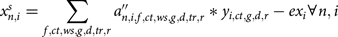 $$x_{n,i}^s = \mathop \sum \limits_{f,ct,ws,g,d,tr,r} {a''_{n,i,f,ct,ws,g,d,tr,r}}*{y_{i,ct,g,d,r}} - e{x_i}\forall n,i$$
Following the FSMA guidelines, equation (8) uses the GM and STV criteria to impose a delay in harvest of up to four days based on a 0.5 log per day microbial die-off (FDA 2014).
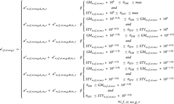 $${\eqalign{ & {{a'}_{i,f,ct,ws,g,r\;}} = \left\{ {\matrix{ {{{a''}_{n,i,f,ct,ws,g,{d_0},t{r_0},r}}} \hfill & if{\left\{ {\matrix{ \matrix{ G{M_{n,i,f,ct,ws,r}}{\rm{\;}}*\;{10^0}\;\;\; \le \;{\theta _{GM}}{\rm{\;}}\; \le max \hfill \cr {\quad\quad\quad\quad\quad\quad\quad{and}} \hfill \cr} \hfill \cr {ST{V_{n,i,f,ct,ws,r}}{\rm{\;}}*\;{{10}^0} \le \;{\theta _{STV}}{\rm{\;}} \le max} \hfill \cr } } \right.} \hfill \cr {{{a''}_{n,i,f,ct,ws,g,{d_1},t{r_0},r}} + \;{{a''}_{n,i,f,ct,ws,g,d0,t{r_1},r}}} \hfill & if{\left\{ {\matrix{ \matrix{ G{M_{n,i,f,ct,ws,r}}{\rm{\;}}*\;{10^{\left( { - 0.5} \right)}}\;\;\; \le \;{\theta _{GM}}{\rm{\;}} \le G{M_{n,i,f,ct,ws,r}}{\rm{\;}}*\;{10^0} \hfill \cr \quad\quad\quad\quad\quad\quad\quad\quad\quad\quad\quad{{and}} \hfill \cr} \hfill \cr {ST{V_{n,i,f,ct,ws,r}}*\;{{10}^{\left( { - 0.5} \right)}}\;\;\; \le \;{\theta _{STV}}{\rm{\;}} \le ST{V_{n,i,f,ct,ws,r}}{\rm{\;}}*\;{{10}^0}} \hfill \cr } } \right.} \hfill \cr {{{a''}_{n,i,f,ct,ws,g,{d_2},t{r_0},r}} + \;{{a''}_{n,i,f,ct,ws,g,d0,t{r_1},r}}} \hfill & if{\left\{ {\matrix{ \matrix{ G{M_{n,i,f,ct,ws,r}}{\rm{\;}}*\;{10^{\left( { - 1.0} \right)}}\;\;\;\; \le \;{\theta _{GM}}{\rm{\;}} \le G{M_{n,i,f,ct,ws,r}}{\rm{\;}}*\;{10^{\left( { - 0.5} \right)}} \hfill \cr {\quad\quad\quad\quad\quad\quad\quad\quad\quad\quad\quad{and}} \hfill \cr} \hfill \cr {ST{V_{n,i,f,ct,ws,r}}*\;{{10}^{\left( { - 1.0} \right)}}\;\;\; \le \;{\theta _{STV}}{\rm{\;}} \le ST{V_{n,i,f,ct,ws,r}}{\rm{\;}}*\;{{10}^{\left( { - 0.5} \right)}}} \hfill \cr } } \right.} \hfill \cr {{{a''}_{n,i,f,ct,ws,g,{d_3},t{r_0}r}} + \;{{a''}_{n,i,f,ct,ws,g,d0,t{r_1},r}}} \hfill & if{\left\{ {\matrix{ \matrix{ G{M_{n,i,f,ct,ws,r}}{\rm{\;}}*\;{10^{\left( { - 1.5} \right)}}\;\;\;\; \le {\theta _{GM}}{\rm{\;}} \le G{M_{n,i,f,ct,ws,r}}{\rm{\;}}*\;{10^{\left( { - 1.0} \right)}} \hfill \cr {\quad\quad\quad\quad\quad\quad\quad\quad\quad\quad\quad{and}} \hfill \cr} \hfill \cr {ST{V_{n,i,f,ct,ws,r}}*\;{{10}^{\left( { - 1.5} \right)}}\;\;\; \le \;{\theta _{STV}}{\rm{\;}} \le ST{V_{n,i,f,ct,ws,r}}{\rm{\;}}*\;{{10}^{\left( { - 1.0} \right)}}} \hfill \cr } } \right.} \hfill \cr {{{a''}_{n,i,f,ct,ws,g,{d_4},t{r_0},r}} + \;{{a''}_{n,i,f,ct,ws,g,d0,t{r_1},r}}} \hfill & if{\left\{ {\matrix{ \matrix{ G{M_{n,i,f,ct,ws,r}}{\rm{\;}}*\;{10^{\left( { - 2.0} \right)}}\;\;\;\; \le {\theta _{GM}}{\rm{\;}} \le G{M_{n,i,f,ct,ws,r}}{\rm{\;}}*\;{10^{\left( { - 1.5} \right)}} \hfill \cr {\quad\quad\quad\quad\quad\quad\quad\quad\quad\quad\quad{and}} \hfill \cr} \hfill \cr {ST{V_{n,i,f,ct,ws,r}}*\;{{10}^{\left( { - 2.0} \right)}}\;\;\; \le \;{\theta _{STV}}{\rm{\;}} \le ST{V_{n,i,f,ct,ws,r}}{\rm{\;}}*\;{{10}^{\left( { - 1.5} \right)}}} \hfill \cr } } \right.} \hfill \cr {{{a''}_{n,i,f,ct,ws,g,{d_5},t{r_0},r}} + \;{{a''}_{n,i,f,ct,ws,g,d0,t{r_1},r}}} \hfill & if{\left\{ {\matrix{ \matrix{ {\theta _{GM}}{\rm{\;}} \le G{M_{n,i,f,ct,ws,r}}{\rm{\;}}*\;{10^{\left( { - 2.0} \right)}} \hfill \cr {\quad\quad\quad\quad\quad\quad{and}} \hfill \cr} \hfill \cr {{\theta _{STV}}{\rm{\;}} \le ST{V_{n,i,f,ct,ws,r}}{\rm{\;}}*\;{{10}^{\left( { - 2.0} \right)}}} \hfill \cr } } \right.} \hfill \cr } } \right. \cr & \quad\quad\quad\quad\quad\quad\quad\quad\quad\quad\quad\quad\quad\quad\quad\quad\quad\quad\quad\quad\quad\quad\quad\quad\quad\quad\quad\quad\quad\quad\quad\quad\quad\forall i,f,ct,ws,g,r\; \cr}} $$
The FSMA regulatory standard (equation 8) requires: (1) ${\theta _{GM}}$
of 126 or less CFU per 100 ml of water, and (2)
${\theta _{GM}}$
of 126 or less CFU per 100 ml of water, and (2) ${\theta _{STV}}$
of 410 or less CFU (FDA 2014). If either criterion is violated, farmers must cease irrigating from the contaminated source, delay harvest to allow for microbial die-off, or treat irrigation water (FDA 2014). According to the FSMA guidelines, harvest can be delayed for up to four days. Produce that is not in compliance even after four additional days of microbial die-off, based on the 0.5 log rate reduction of CFUs per day, is to be discarded. The optimal solutions are obtained by iteratively varying standard stringency,
${\theta _{STV}}$
of 410 or less CFU (FDA 2014). If either criterion is violated, farmers must cease irrigating from the contaminated source, delay harvest to allow for microbial die-off, or treat irrigation water (FDA 2014). According to the FSMA guidelines, harvest can be delayed for up to four days. Produce that is not in compliance even after four additional days of microbial die-off, based on the 0.5 log rate reduction of CFUs per day, is to be discarded. The optimal solutions are obtained by iteratively varying standard stringency, $\;{\theta _{GM}}$
and
$\;{\theta _{GM}}$
and ${\theta _{STV}}$
, proportionally. This approach is used in place of solving the model for
${\theta _{STV}}$
, proportionally. This approach is used in place of solving the model for ${\theta _{GM}}$
and
${\theta _{GM}}$
and ${\theta _{TV}}$
as endogenously determined variables to minimize nonlinearity of the model and reduce computational complexity.
${\theta _{TV}}$
as endogenously determined variables to minimize nonlinearity of the model and reduce computational complexity.
Following LGMA guidelines, equation (8') uses the CFUs of water quality samples to impose water treatment.
 $${a'_{i,f,ct,ws,g,r\;}} = \left\{ {\matrix{ {{{a''}_{n,i,f,ct,ws,g,d0,t{r_0},r}}} \hfill \quad if& {G{M^{\prime}}_{n,i,f,ct,ws,g,r}{\rm{\;}} \le \;\theta '{\rm{\;}}\; \le max} \hfill \cr {{{a''}_{n,i,f,ct,ws,g,d0,t{r_1},r}}} \hfill \quad if& {G{M^{\prime}}_{n,i,f,ct,ws,g,r}{\rm{\;}} \ge \;\theta '} \hfill \cr } } \right.\quad \forall i,f,ct,ws,g,r.$$
where $\theta '$
is the LGMA water quality standard, 126 CFU/100 ml of irrigation water (California Leafy-Greens Marketing Agreements 2020).
$\theta '$
is the LGMA water quality standard, 126 CFU/100 ml of irrigation water (California Leafy-Greens Marketing Agreements 2020). $G{M^{\prime}}_{n,i,f,ct,wsg,r}$
is the irrigation-event-specific geometric mean (California Leafy-Greens Marketing Agreements 2020).
$G{M^{\prime}}_{n,i,f,ct,wsg,r}$
is the irrigation-event-specific geometric mean (California Leafy-Greens Marketing Agreements 2020).
Each day of delay in harvest is assumed to reduce yield by a fixed share ( $\pi )\;$
until the fifth day, when produce is discarded.Footnote
8
Hence, the per acre yield is expressed as follows (equation 9) where d is days of delay in harvest (e.g.,
$\pi )\;$
until the fifth day, when produce is discarded.Footnote
8
Hence, the per acre yield is expressed as follows (equation 9) where d is days of delay in harvest (e.g., ${d_0}$
indicates no delay,
${d_0}$
indicates no delay, ${d_1}$
represents 1 day of delay, etc.), and
${d_1}$
represents 1 day of delay, etc.), and ${\mathord{\buildrel{\lower3pt\hbox{$\scriptscriptstyle\smile$}} \over y} _{i,ct,g}}$
is average observed yield of crop i in county ct with no delay.
${\mathord{\buildrel{\lower3pt\hbox{$\scriptscriptstyle\smile$}} \over y} _{i,ct,g}}$
is average observed yield of crop i in county ct with no delay.
 $$\left\{ {\matrix{ {{y_{i,c,g,d,r}} = {{\mathord{\buildrel{\lower3pt\hbox{$\scriptscriptstyle\smile$}}\over y} }_{i,ct,g}}*\left( {1 - \pi d} \right)\;\;\;\;\;\;\;\;\;if\;d = {d_0},\;{d_1},\;{d_2},{d_3},\;{d_4}} \cr {{y_{i,ct,g,d,r}} = 0\;\;\;\;\;\;\;\;\;\;\;\;\;\;\;\;\;\;\;\;\;\;\;\;\;\;\;\;\;\;\;\;\;\;\;if\;d = \;{d_5}\;\;\;\;\;\;\;\;\;\;\;} \cr } \;\;\;\;\;\;\;\;\;\;\;\;\;\;\;\;\forall i,ct,g,r} \right.$$
Equations (10) and (11) estimate the GM and STV values across production districts and farm types in each state of nature (Bihn et al. Reference Bihn, Fick, Pahl, Stoeckel, Woods and Wall2017).
 $$G{M_{n,i,f,ct,ws,r}} = {10^{\left\{ {\matrix{ {\{ \mathop \sum \nolimits_{t'} \log \left( {C{P_{n,i,f,ct,ws,t',r}}} \right)} \cr + \cr {\mathop \sum \limits_{g' \le g} tes{t_{i,f,ct,ws,g,g',r}}*\log \left( {{C_{n,i,f,ct,ws,g',r}}} \right)\} /{\rm{\Lambda }}\left( {ws} \right)} \cr } } \right\}}}\;\;\forall n,i,f,ct,ws,r\;$$
 $$ST{V_{n,i,f,ct,ws,r}} = \;{10^{\left( {G{M_{n,i,f,ct,ws,r}} + 1.282*ST{D_{n,i,f,ct,ws,r}}} \right)}}\;\;\;\;\;\;\;\;\;\;\;\;\;\;\;\;\;\;\;\;\;\;\;\;\;\;\;\;\;\;\forall n,i,f,ct,ws,r$$
where ${C_{n,i,f,ct,ws,g,r}}$
is E. coli CFU per 100 ml of irrigation water, and
${C_{n,i,f,ct,ws,g,r}}$
is E. coli CFU per 100 ml of irrigation water, and $C{P_{n,i,ct,f,ws,t',r}}$
is E. coli CFU per 100 ml from irrigation in the months prior to the last month of the growing season (t')Footnote
9
as part of the Microbial Water Quality Profile (MWQP).
$C{P_{n,i,ct,f,ws,t',r}}$
is E. coli CFU per 100 ml from irrigation in the months prior to the last month of the growing season (t')Footnote
9
as part of the Microbial Water Quality Profile (MWQP). $\;ST{D_{n,i,f,ct,ws,r}}$
is the combined standard deviation of
$\;ST{D_{n,i,f,ct,ws,r}}$
is the combined standard deviation of $\log \left( {{C_{n,i,f,ct,ws,g',r}}} \right)$
and
$\log \left( {{C_{n,i,f,ct,ws,g',r}}} \right)$
and $\log \left( {C{P_{n,i,f,ct,ws,t',r}}} \right)$
.
$\log \left( {C{P_{n,i,f,ct,ws,t',r}}} \right)$
. $g'$
refers to the preceding and current irrigation events.Footnote
10
GM and STV are estimated based on the aggregate CFUs of generic E. coli across irrigation events.
$g'$
refers to the preceding and current irrigation events.Footnote
10
GM and STV are estimated based on the aggregate CFUs of generic E. coli across irrigation events. ${\rm{\Lambda }}$
(ws) is the number of surface and groundwater samples. The initial MWQP is to be based on at least twenty surface water samples and at least four groundwater samples. In subsequent years, five (one) samples of surface (ground) water in the last month of irrigation are required to update MWQP (FDA 2020).
${\rm{\Lambda }}$
(ws) is the number of surface and groundwater samples. The initial MWQP is to be based on at least twenty surface water samples and at least four groundwater samples. In subsequent years, five (one) samples of surface (ground) water in the last month of irrigation are required to update MWQP (FDA 2020).
E. coli content of irrigation water $(C{O_{n,i,f,ct,ws,g,r}})$
is stochastic:
$(C{O_{n,i,f,ct,ws,g,r}})$
is stochastic:
 $$C{O_{n,i,f,ct,ws,g,r}} = Max\left\{ {\left( {0,{\rm{\Omega }}\left( {{k_1},\;{k_2}} \right)} \right)} \right\}\forall n,i,f,ct,ws,g,r$$
where ${\rm{\Omega \;}}$
is the Lognormal or Weibull distribution and (k
1
, k
2
) are the scale and shape parameters.
${\rm{\Omega \;}}$
is the Lognormal or Weibull distribution and (k
1
, k
2
) are the scale and shape parameters.
E. coli O157:H7 transmits from irrigation water to crops according to equation (13), where CFUs from all irrigation events are aggregated and adjusted to reflect die-off including from delays in harvest in FSMA scenarios. LGMA recognizes several methods for water treatment including physical devices such as heat sterilization and ultraviolet light (UV) and chemicals like chlorine dioxide or peroxyacetic acid (Rock Reference Rock2020). Following Krishnan et al. (Reference Krishnan, Kogan, Peters, Thomas and Critzer2021), we assume that applying chlorine to water is the most common agricultural water treatment method. According to the CDC (2022a) adding 0.5 mg/l free chlorine to water for less than 30 minutes reduces the concentration of E. coli by 99.99%. Crop irrigation water consumption is determined by irrigation efficiency (λ) (evapotranspiration divided by applied water per acre). Hence, the amount of E. coli in lettuce after irrigation is proportional to consumptive use (Solomon et al. Reference Solomon, Potenski and Matthews2002).Footnote 11 Irrigation efficiency varies across irrigation methods. California and Arizona lettuce producers mostly use pressurized furrow irrigation technology (FDA 2016).
 $$C{N_{n,i,f,ct,ws,g,d,tr,r}} = \mathop \sum \nolimits_{g' \le g} \left( {{{C{O_{n,i,f,ct,ws,g',r}}} \over {100}}} \right)*\lambda *R*0.96*{e^{ - {{{{l\left( {g'} \right)} \over \varepsilon }}^\zeta }}}*{10^{ - 0.5*d}}\; \\ *{10^{ - 4\left\{ {tr - 1} \right\}}}*\eta \,\forall n,i,f,ct,ws,g,d,tr,r$$
An exponential microbial die-off function ( ${e^{ - {{{{l\left( {g'} \right)} \over \varepsilon }}^\zeta }}}$
) (Brouwer et al. Reference Brouwer, Eisenberg, Remais, Collender, Meza and Eisenberg2017) quantifies the decay of E. coli CFUs from irrigation events to harvest.
${e^{ - {{{{l\left( {g'} \right)} \over \varepsilon }}^\zeta }}}$
) (Brouwer et al. Reference Brouwer, Eisenberg, Remais, Collender, Meza and Eisenberg2017) quantifies the decay of E. coli CFUs from irrigation events to harvest. $l\left( {g'} \right)$
represents the number of days between each irrigation event and the final irrigation before harvest.
$l\left( {g'} \right)$
represents the number of days between each irrigation event and the final irrigation before harvest.
E. coli O157:H7 is the primary E. coli strain that causes foodborne illness outbreaks (CDC 2020). Therefore, based on the availability of O157:H7 prevalence data relative to Generic E. coli, in the baseline scenario, we focus on E. coli O157:H7 (Muniesa et al. Reference Muniesa, Jofre, García-Aljaro and Blanch2006; Ottoson et al. Reference Ottoson, Nyberg, Lindqvist and Albihn2011; Pang et al. Reference Pang, Lambertini, Buchanan, Schaffner and Pradhan2017). However, foodborne illnesses can also be caused by other pathogens such as E. coli O26, O45, O103, O111, O121, and O145 (Bertoldi et al. Reference Bertoldi, Richardson, Schneider, Kurdmongkolthan and Schneider2018). We vary (R) in the sensitivity analysis to examine how water pathogenicity affects optimal water quality standard.
Following Pang et al. (Reference Pang, Lambertini, Buchanan, Schaffner and Pradhan2017), it is assumed that fresh lettuce remains in storage and transportation for 4 days after harvest before consumption, with associated microbial die-off.Footnote 12 The microbial die-off during storage, transportation, and retail is modeled using an exponential form (Pang et al. Reference Pang, Lambertini, Buchanan, Schaffner and Pradhan2017):
 $$CN{S_{n,i,f,ct,ws,g,d,tr,r}} = C{N_{n,i,f,ct,ws,g,d,tr,r}}\;*\;{e^{ - \left( {\rm U*4*24} \right)}}\;\;\;\;\;\;\;\;\;\;\;\;\;\;\;\forall n,i,f,ct,ws,g,tr,r\;$$
where $CN{S_{n,i,f,ct,ws,g,d,tr,r}}\;$
is CFUs of E. coli in crop after transportation, storage, and retail and before consumption. Ʋ is the average hourly die-off rate per CFU of E. coli.
$CN{S_{n,i,f,ct,ws,g,d,tr,r}}\;$
is CFUs of E. coli in crop after transportation, storage, and retail and before consumption. Ʋ is the average hourly die-off rate per CFU of E. coli.
The dose–response formulation is adopted from Pang et al. (Reference Pang, Lambertini, Buchanan, Schaffner and Pradhan2017). Serving size ( ${\varrho _i}$
) and pathogen quantity per gram of produce after the delay in harvest are used to estimate E. coli dose (
${\varrho _i}$
) and pathogen quantity per gram of produce after the delay in harvest are used to estimate E. coli dose ( ${D_{n,i,f,ct,ws,g,d,tr,r}}$
) per contaminated serving (equation 15). A dose–response relation (16) estimates the probability (
${D_{n,i,f,ct,ws,g,d,tr,r}}$
) per contaminated serving (equation 15). A dose–response relation (16) estimates the probability ( ${p_{n,i,f,ct,ws,g,d,tr,r}}$
) of illness per contaminated serving, where
${p_{n,i,f,ct,ws,g,d,tr,r}}$
) of illness per contaminated serving, where $\rho $
and
$\rho $
and $\omega $
are dose–response parameters (Pang et al. Reference Pang, Lambertini, Buchanan, Schaffner and Pradhan2017). Illnesses are calculated based on the probability of illness per contaminated serving (17).Footnote
13
$\omega $
are dose–response parameters (Pang et al. Reference Pang, Lambertini, Buchanan, Schaffner and Pradhan2017). Illnesses are calculated based on the probability of illness per contaminated serving (17).Footnote
13
In equation (16), $\alpha $
is the impact of distributors, retailers, and consumers’ prevention efforts. Formulation in equation (16) implies substitution between prevention efforts and regulatory stringency
$\alpha $
is the impact of distributors, retailers, and consumers’ prevention efforts. Formulation in equation (16) implies substitution between prevention efforts and regulatory stringency $({S_{\theta \alpha }}$
<0). An alternative formulation
$({S_{\theta \alpha }}$
<0). An alternative formulation ${p_{n,i,f,ct,ws,g,d,tr,r}} = 1 - {\left( {1 + \;{{{D_{n,i,f,ct,ws,g,d,tr,r}}} \over {\alpha *\omega }}} \right)^{ - \rho }}$
can be used for complementarity
${p_{n,i,f,ct,ws,g,d,tr,r}} = 1 - {\left( {1 + \;{{{D_{n,i,f,ct,ws,g,d,tr,r}}} \over {\alpha *\omega }}} \right)^{ - \rho }}$
can be used for complementarity $({S_{\theta \alpha }}$
>0), which is unlikely in our case.
$({S_{\theta \alpha }}$
>0), which is unlikely in our case.
 $${D_{n,i,f,ct,ws,g,d,tr,r}} = CN{S_{n,i,f,ct,ws,g,d,tr,r}}*{\varrho _i}\forall n,i,f,ct,ws,g,d,tr,r$$
 $${p_{n,i,f,ct,ws,g,d,tr,r}} = \left[ {1 - {{\left( {1 + \;{{{D_{n,i,f,ct,ws,g,d,tr,r}}} \over \omega }} \right)}^{ - \rho }}} \right]*\left( {{1 \over \alpha }} \right)\forall n,i,f,ct,ws,g,d,tr,r$$
 $$il{l_n} = \mathop \sum \limits_{i,f,ct,ws,g,d,t,r} {p_{n,i,f,ct,ws,g,d,tr,tr,r}}*{a''_{n,i,f,ct,ws,g,d,tr,r}}*\;{y_{i,ct,g,d,r}}*{{50,802.3} \over {{\varrho _i}}}\forall n$$
We assume that foodborne outbreaks result in negative demand shocks. The demand response is assumed to be a function of the number of foodborne illnesses (equation 18). $\aleph $
is the median reduction in demand per illness in each state of nature and is obtained according to Bovay and Sumner (Reference Bovay and Sumner2017) and Arnade et al. (Reference Arnade, Calvin and Kuchler2009) (see Appendix B).
$\aleph $
is the median reduction in demand per illness in each state of nature and is obtained according to Bovay and Sumner (Reference Bovay and Sumner2017) and Arnade et al. (Reference Arnade, Calvin and Kuchler2009) (see Appendix B).
 $${\varpi _n} = \aleph *\;il{l_n}\forall n$$
Data
The empirical analysis focuses on the microbial irrigation water quality in lettuce production. Lettuce is of particular interest for food safety because all lettuce is consumed fresh without further processing. Also, unlike other fresh vegetables, lettuce is highly perishable, limiting the opportunity for storage and microbial die-off before consumption. Forty-three counties in California and Arizona produce nearly all U.S. Head and Leaf-Romaine lettuce (U.S. Department of Agriculture 2018). In 2017, Head and Leaf-Romaine lettuce were planted on approximately 18,194 and 48,964 acres in California and Arizona, respectively.
The cost burden of FSMA regulations falls disproportionately on small farms due to economies of scale (Lichtenberg and Page Reference Lichtenberg and Page2016; Bovay and Sumner Reference Bovay and Sumner2017; Adalja and Lichtenberg Reference Adalja and Lichtenberg2018; Bovay et al. Reference Bovay, Ferrier and Zhen2018). Therefore, farms are categorized into small, gross income less than $250,000, and large, gross income greater than $250,000 (U.S. Department of Agriculture 2017) to account for scale economies. The costs of implementing the water quality standards based on GM and STV criteria are obtained from the FDA (2015b) and include water sampling, testing, and recordkeeping costs. Similarly, water treatment costs in LGMA and FSMA are estimated using FDA (2015b). In particular, the baseline water treatment costs are estimated at $24.76 and $2.48 per acre for small and large lettuce producing farms, respectively. Calvin et al. (Reference Calvin, Jensen, Klonsky and Cook2017) also provide estimates of direct irrigation water treatment costs. However, their estimated costs are presented per firm rather than per acre. Hence, we rely on the FDA’s cost estimates. Production, consumption, planted acreage, prices, import, export, and applied irrigation water data for lettuce are obtained from U.S. Department of Agriculture (USDA) ERS and NASS.
The FDA estimates that the microbial irrigation water quality standard implementation for domestic farms costs $50 million annually (FDA 2015b). This estimate includes water sampling, testing, and recordkeeping costs. Adjusting this estimate based on the share of harvested lettuce acreage relative to all fresh fruits and vegetables acres, the cost for the lettuce industry is approximately $3 million annually.
Costs per foodborne illness vary depending on the severity of the disease and estimation methodology. USDA (2019) uses $8,500 per illness caused by E. coli O157:H7. Hammitt and Haninger (Reference Hammitt and Haninger2007) estimates willingness to pay (WTP) to avoid foodborne illness between ten and twenty thousand dollars. We use $8,500, following USDA as a baseline value, but rely on Hammitt and Haninger (Reference Hammitt and Haninger2007) values in the sensitivity analysis.
Own-price elasticity of demand (Okrent and Alston Reference Okrent and Alston2012),Footnote 14 cross-price elasticities of demand (Ferrier et al. Reference Ferrier, Zhen and Bovay2016), and own-price elasticity of supply (Lohr and Park Reference Lohr and Park1992) are provided in the appendix (Table B.3). The average of the cross-price elasticities between Head and Leaf and Head and Romaine is used as the proxy for the cross-price elasticity between Head lettuce and the combined Leaf-Romaine lettuce. A similar assumption applies to the Leaf-Romaine and Head lettuce cross-price elasticity.
Spatial microbial water quality data for Generic E. coli are obtained from the National Water Quality Monitoring Council (USGS-EPA 2020).Footnote 15 The reported Generic E. coli water quality ranges from 32 CFU per 100 ml in San Joaquin county to 5,931 in Ventura county. Density plots, Q-Q plots, P-P plots, and Akaike Information Criteria (AIC) are used to select the best distribution function for each county using the data from NWIS and STORET Databases. E. coli content in groundwater is only available for three counties for which we use Weibull distribution functions. For the rest of the counties, the corresponding surface water distribution functions are shifted to the left to obtain groundwater quality distribution. The shift parameter is the average ratio of the means of surface and groundwater distributions in the counties where the data are available for both sources. Generic E. coli data are absent for 17 smaller counties in California. Data for these counties are obtained from the neighboring counties. The same density functions are used to obtain random draws for production districts located within a county. Five hundred random draws in each production district are used per model solution for microbial water quality data. Mean values of E. coli CFU/100 ml across counties are provided in Appendix Figure B.1.
Results
The empirical model is validated by reproducing observed prices and quantities in the past under baseline conditions. Annual results from 2008 to 2017 are reproduced using county crop acreage data from the corresponding years. Model solutions produce lettuce quantities and prices within 1% and 5% of the observed data in the corresponding year (Table B.4). These validation results provide a solid foundation for FSMA scenario analysis. The policy analyses are based on the supply and demand functions calibrated to the prices and quantities observed in 2016. Planted acreage is subject to synthetic and observed crop mix data from all available years. Hence, the model solutions represent a long-run market equilibrium.
Table 1 shows results from two scenarios corresponding to baseline and high water treatment costs. Each of these cases includes four subscenarios corresponding to FSMA-mandated, optimal FSMA, LGMA-mandated, and optimal LGMA standards. The FSMA mandate scenario uses fixed water quality threshold values ( ${\theta _{GM}}$
and
${\theta _{GM}}$
and ${\theta _{STV}})$
as required by the FDA rule (126 CFU/100 ml for GM and 410 CFU/100 ml for STV). Similarly, the LGMA mandate scenario has the same GM threshold. The optimal FSMA and LGMA scenarios provide solutions with endogenously determined thresholds for microbial water quality standards that generate the greatest objective function value.
${\theta _{STV}})$
as required by the FDA rule (126 CFU/100 ml for GM and 410 CFU/100 ml for STV). Similarly, the LGMA mandate scenario has the same GM threshold. The optimal FSMA and LGMA scenarios provide solutions with endogenously determined thresholds for microbial water quality standards that generate the greatest objective function value.
Regulatory standard, welfare, illnesses, and lettuce prices
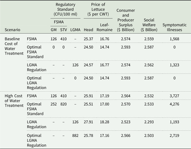
Notes: FSMA and LGMA stand for Food Safety Modernization Act and Leafy-Greens Marketing Agreement, respectively.
There are three reasons for including the high treatment cost scenario in this study. First, the baseline cost of water treatment in the FDA (2015b) includes only labor and material costs. However, the use of chemicals such as chlorine for treating irrigation water can increase plant phytotoxicity and create toxic by-products, e.g., haloacetic acid and trihalomethanes (Raudales et al. Reference Raudales, Parke, Guy and Fisher2014; Dery et al. Reference Dery, Brassill and Rock2020). These by-products can be harmful for human health (Deborde and von Gunten Reference Deborde and Von Gunten2008; Raudales et al. Reference Raudales, Parke, Guy and Fisher2014) and to environment. Second, treatment chemicals can degrade lettuce quality as excess cholerine can accumulate in crop tissues, resulting in crop leaves with a burned or scorched appearance (University of Maryland Extension 2022). Third, only two estimates of irrigation water treatment costs are available (FDA 2015b; Calvin et al. Reference Calvin, Jensen, Klonsky and Cook2017), which suggests uncertainty about the costs of water treatment. We iteratively increase the water treatment costs until the LGMA treatment is no longer cost effective. The results show that the baseline water treatment costs have to increase 500 times for water treatment to be inferior to harvest delay.
In the low water treatment cost scenario, FSMA regulation produces slightly lower benefits than the LGMA program. The difference is attributed to a greater number of illnesses under FSMA than under LGMA. In the FSMA scenario, small farmers choose to delay harvest rather than treat water when water is contaminated. However, treating water is more effective for preventing illnesses than delaying harvest, which reduces microbial contamination but does not eliminate it. Therefore, the number of symptomatic cases under LGMA is lower than under FSMA. However, even in the LGMA scenario, there are some illnesses because water is treated only if microbial water is worse than the standard of 126 CFUs per 100 ml.
The results show small welfare variation across the scenarios in Table 1. Hence, FSMA regulation does not improve welfare relative to the existing LGMA program. This result is not surprising given a small number of annual lettuce-related foodborne illnesses and associated monetary losses, relative to the value of the lettuce market in terms of aggregate consumer and producer surplus.
In the low-cost water treatment scenario (baseline), the optimal water quality standard is significantly more stringent than the standard mandated under the FSMA and LGMA. This result is expected for the low water treatment cost scenarios because water treatment prevents foodborne illness without sacrificing consumer and producer surplus. If treatment costs are low, then treating water is justified to prevent illness costs. Although water treatment is expensive for small farms even in the low-cost scenario, the benefits of a strict threshold, which prevents more illnesses, outweigh the treatment costs for small farms.
On the other hand, the optimal water quality standard is less stringent than the FSMA and LGMA requirements in the high-water treatment cost scenario. In this case, delaying harvest under FSMA is preferred to treatment. However, harvest delays are costly due to consumer and producer surplus losses. Therefore, the optimal FSMA standard is less stringent than the FSMA rule.
In the high treatment cost scenario, the LGMA objective function value is 9.4% (2.293/2.532) lower than the FSMA value. Similarly, the optimal LGMA objective function is 1.2% (2.503/2.533) lower than the optimal FSMA value. The dominance of FSMA relative to LGMA is not surprising since the high treatment cost scenario is designed to increase treatment costs until treating water is no longer optimal relative to harvest delay. Therefore, the addition of harvest delay as an option under FSMA can improve efficiency relative to LGMA if water treatment costs are substantially (at least 500 times) higher than in the baseline scenario. However, the difference in social welfare between corresponding FSMA and LGMA scenarios is still small.
FDA estimated $310 million in annual benefits of FSMA irrigation water quality standards from avoided foodborne illnesses (2015b). Our baseline estimates suggest that FSMA water quality regulation decreases welfare by $34 ($61) million in a low (high) water treatment cost scenario. The results differ because our estimates a) account for changes in consumer and producer surplus from production and planting decisions and b) are benchmarked against the LGMA program.
As expected, there is an inverse relationship between water quality standard stringency and the number of foodborne illnesses in both treatment cost scenarios. In the high treatment cost scenario, doubling the microbial quality limit in the FSMA, which implies less stringent regulation, produces 14.7% more illnesses in the optimal FSMA scenario (4,276/3,727). Similarly, in the LGMA standard, higher microbial water quality limit increases illnesses. However, since the cost of water treatment is prohibitively expensive, the social welfare improves relative to the mandated requirement under FSMA despite the increase in the number of symptomatic illnesses.
In the baseline treatment cost scenario, FSMA results in 3.3% higher Head (25.37/24.57) and 0.1% lower Leaf-Romaine (16.76/16.77) lettuce prices, respectively, relative to LGMA outcomes. The changes in prices are due to a) long run acreage adjustment in response to the regulatory requirements and b) supply losses due to harvest delays in the FSMA scenario. As expected, prices do not change across FSMA and LGMA scenarios with optimized microbial water quantity threshold. In the high treatment cost scenario, prices are lower in the FSMA than in the LGMA solutions. Higher prices in the LGMA scenario are due to the decrease in the long run crop acreage in response to expensive and mandatory water treatment.
Foodborne illness estimates include all incidents that range from mild discomfort to life-threatening cases. Our illness estimates are comparable to Pang et al. (Reference Pang, Lambertini, Buchanan, Schaffner and Pradhan2017), who estimate 2,160 to 9,320 annual foodborne illnesses on average from contaminated lettuce via irrigation water. The CDC’s reports indicate that 167 people were ill due to E. coli lettuce contamination in 2019 (CDC 2021). However, the CDC shows only the reported cases, while our estimates include total symptomatic cases, some of which are mild and most are unreported. In practice, only 1 in 26 symptomatic cases is reported (Scallan et al. Reference Scallan, Griffin, Angulo, Tauxe and Hoekstra2011; Scharff et al. Reference Scharff, Besser, Sharp, Jones, Peter and Hedberg2016). Accounting for underreporting in CDC records, our estimates are consistent with the reported illness data in 2019.
We evaluate the distribution of FSMA impacts on small versus large lettuce producing farms and on farms that rely on the surface versus groundwater. The results in Table 2 show that in the baseline treatment cost scenario, large and small farms decrease supply by 7.43%, and their revenues increase by 0.42%.Footnote 16 The increase in producer revenue is due to the increase in lettuce prices under FSMA scenario. A qualitatively similar positive effect on revenues is observed in the high water treatment cost scenario, where small and large farms decrease production by 9.56% and 8.91%, while their revenues increase by 0.49% and 1.19%. The results show a relative disadvantage of small farms, which is similar to Bovay and Sumner (Reference Bovay and Sumner2017), who show that FSMA increases (decreases) revenues of large (small) farms by 7%–9% (8%–29%).
FSMA impacts on small and large farms as well as ground and surface water using farms
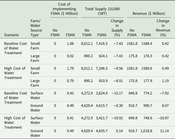
A comparison of impacts on farms that use surface versus groundwater reveals that, as expected, FSMA affects surface water producers more than groundwater producers (Table 2). In the baseline treatment cost scenario, surface (ground) water farms’ supply decreases by 15.17% (0.3%), with a corresponding 7.92% decrease (8.07% increase) in total revenue. In the high treatment cost scenario, surface (ground) water farms decrease (increase) production by 19.92% (0.14%), which results in a 10.97% (11.14%) decrease (increase) in revenues. The asymmetric effect of FSMA is expected because groundwater is less contaminated and is less stringently regulated. As a result, some production shifts from surface to groundwater irrigation.
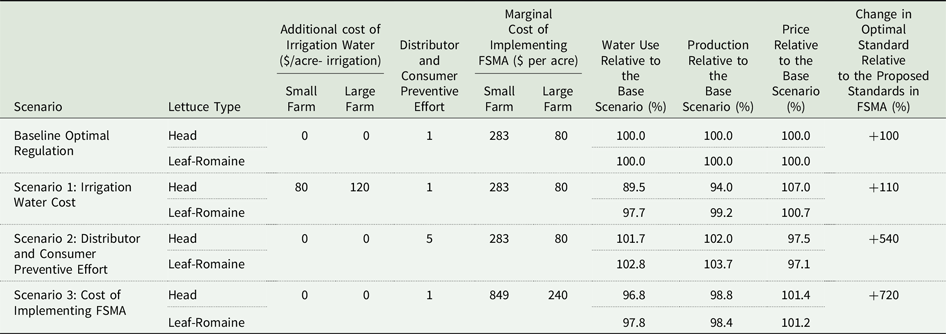
We empirically examine the effect of irrigation water cost (proposition a), contamination prevention efforts by consumers and producers (proposition b), and FSMA compliance cost (proposition c) on optimal water quality standard and water use in the high water treatment cost scenario. According to proposition a), more costly irrigation is expected to reduce irrigation and stringency of microbial water quality standard. Irrigation costs decrease production, which increases the marginal value of output. Also, lower production results in fewer illnesses. Hence, optimal standard stringency decreases. We examine this effect empirically by varying the cost of irrigation water. In the baseline scenario (Table 3), water-related costs are included in the per acre marginal production costs. In scenario 1, the additional irrigation costs are increased to $80 and $120 for small and large farms, respectively, per irrigation event per acre.Footnote 17 Although irrigation is price inelastic (Scheierling et al. Reference Scheierling, Loomis and Young2006), with a sufficiently large increase in irrigation costs, water use decreases, and so does the stringency of optimal water quality standard. A twenty-fold increase in irrigation costs to $80 and $120 for small and large farms reduces water use by 10.5% and 2.3% in Head and Leaf-Romaine lettuce production, respectively. As a result, the production of Head and Leaf-Romaine lettuce decreases by 6% and 0.8%, respectively. With less irrigation and lower output, E. coli contamination decreases, which results in fewer cases of foodborne illnesses. Consequently, with smaller expected damages from foodborne illnesses, the stringency of water quality standard decreases. Relative to the baseline scenario, regulatory stringency in scenario 1 decreases by 10%.
Effects of changes in irrigation costs, distributor and consumer preventive efforts, and cost of implementing the FSMA standard in the high water treatment cost environment
Notes: Scenario (1) shows the results of an increase in irrigation cost relative to the baseline scenario. Scenarios (2) and (3) show the impacts of an increase in distributor and consumer preventive efforts and cost of implementing the FSMA standard on optimal water quality standard, production, price, and water use.
Proposition b) says that distributor and consumer prevention efforts have an ambiguous effect on the optimal water quality standard and irrigation when regulatory stringency and prevention efforts are substitutes. Substitution may arise when distributor and consumer efforts decrease the effectiveness of the quality standard and vice versa. For example, under strict food safety standards, consumers may be less inclined to wash fresh produce before eating. Our empirical results (Table 3, scenario 2) show that a five-fold decrease in the probability of illness due to greater distributor or consumer prevention efforts results in less stringent water quality standard, greater irrigation, increase in production by 2–3.7%, and a decrease in prices of Head and Leaf Romain lettuce by 2.5 and 2.9%, respectively. When consumers or distributors exert more effort to prevent foodborne outbreaks, the probability and the number of foodborne illnesses decrease. As a result, production expands, and the optimal stringency of water quality standard declines.
We empirically examine proposition c) using the high and low costs of FSMA implementation. In scenario 3 (Table 3), costs of FSMA implementation are three times greater than in the baseline. Confirming proposition c), an increase in the standard’s operational costs reduces the standard’s optimal stringency by 720% relative to the optimal regulation scenario with baseline costs. Less stringent standard reduces harvest delay and increases foodborne illnesses. As a result of more foodborne illnesses and associated demand response, production decreases until the marginal cost of additional illness equals marginal benefit of additional lettuce supply in terms of consumer and producer surplus. In our example, Head and Leaf-Romaine lettuce production decreases by approximately 1.2% and 1.6% and prices increase by 1.4% and 1.2%, respectively.
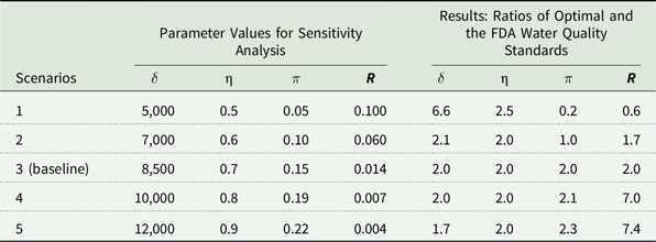
The sensitivity to the key parameters is examined by varying one parameter value at a time, holding others at baseline values. The parameters in the sensitivity analysis and the respective values are provided in the first four columns of Table 4, including the monetary value of foodborne illness damages $\left( \delta \right)$
, the transmission of pathogens from source water to lettuce via irrigation (η), yield loss due to each additional day of delay in harvest (
$\left( \delta \right)$
, the transmission of pathogens from source water to lettuce via irrigation (η), yield loss due to each additional day of delay in harvest ( $\pi $
), and the ratio of harmful pathogens including E. coli O157:H7 to Generic E. coli (R). Scenario 3 is the baseline case in the sensitivity analysis. Sensitivity analysis results are presented in terms of the ratio of the optimal and FDA mandated (GM=126 and STV=410) standard stringencies in the last four columns. A ratio that is greater (less) than 1 suggests less (more) stringent regulation than what is articulated in the FDA rule.
$\pi $
), and the ratio of harmful pathogens including E. coli O157:H7 to Generic E. coli (R). Scenario 3 is the baseline case in the sensitivity analysis. Sensitivity analysis results are presented in terms of the ratio of the optimal and FDA mandated (GM=126 and STV=410) standard stringencies in the last four columns. A ratio that is greater (less) than 1 suggests less (more) stringent regulation than what is articulated in the FDA rule.
Sensitivity analysis for key parameter values
Notes: $\delta $
refers to the economic losses per case of illness; η is the proportion of E. coli in the water source that is delivered to the crop;
$\delta $
refers to the economic losses per case of illness; η is the proportion of E. coli in the water source that is delivered to the crop; $\pi $
is the productivity loss as a result of the delay in harvest by a day; R is the ratio of harmful pathogen presence per CFU of Generic E. coli in irrigation water.
$\pi $
is the productivity loss as a result of the delay in harvest by a day; R is the ratio of harmful pathogen presence per CFU of Generic E. coli in irrigation water.
The results show that the severity of foodborne illness ( $\delta $
) and stringency of water quality standard are positively related. In the baseline scenario, the ratio of optimal and FSMA-mandated standard stringency is 2. If the average cost per illness is $5,000 ($7,000) rather than the baseline $8,500, then the optimal microbial water quality threshold is 6.6 (2.1) times greater than the FSMA regulation. Hence, the greater the cost of foodborne illness, the greater the ex-post damages of water contamination. Therefore, the stringency of water quality standard increases in response to costlier illness to reduce the ex-post damages. Similarly, the greater transmission of pathogens from source water to crop (η) results in a more stringent standard. If the transmission of pathogens from irrigation water to crops decreases from 70% to 50%, then the standard is 2.5 rather than 2 times less stringent than the FDA standard.
$\delta $
) and stringency of water quality standard are positively related. In the baseline scenario, the ratio of optimal and FSMA-mandated standard stringency is 2. If the average cost per illness is $5,000 ($7,000) rather than the baseline $8,500, then the optimal microbial water quality threshold is 6.6 (2.1) times greater than the FSMA regulation. Hence, the greater the cost of foodborne illness, the greater the ex-post damages of water contamination. Therefore, the stringency of water quality standard increases in response to costlier illness to reduce the ex-post damages. Similarly, the greater transmission of pathogens from source water to crop (η) results in a more stringent standard. If the transmission of pathogens from irrigation water to crops decreases from 70% to 50%, then the standard is 2.5 rather than 2 times less stringent than the FDA standard.
We also observe that the magnitude of output loss due to harvest delay influences the optimal standard stringency. For example, if yield loss from the delay in harvest ( $\pi $
) decreases from 15% to 5%, the ratio of the optimal microbial threshold to the FSMA rule threshold changes from 2 to 0.2. Hence, with a 5% yield loss, the optimal water quality standard is more stringent than the FSMA rule. Greater yield loss results in producer and consumer surplus loss due to lower supply and higher prices when the harvest is delayed, which indirectly increases the costs of water quality standard and affects long run planting decisions.Footnote
18
$\pi $
) decreases from 15% to 5%, the ratio of the optimal microbial threshold to the FSMA rule threshold changes from 2 to 0.2. Hence, with a 5% yield loss, the optimal water quality standard is more stringent than the FSMA rule. Greater yield loss results in producer and consumer surplus loss due to lower supply and higher prices when the harvest is delayed, which indirectly increases the costs of water quality standard and affects long run planting decisions.Footnote
18
The results are also sensitive to the pathogenicity of irrigation water per CFU of Generic E. coli. The increase in the ratio (R) represents a greater presence of pathogens, including E. coli O157:H7, per CFU of Generic E. coli. The results show that the stringency of water quality standard increases as the prevalence of pathogens increases. For instance, a ten-fold increase in R increases the stringency of the optimal standard relative to the FDA’s standard.
The sensitivity analysis demonstrates that the FDA water quality standard is not optimal in most scenarios. Eighteen out of twenty scenarios produce less stringent optimal standards than the FDA-mandate. Hence, in most cases, the FDA rule is not economically efficient.
Conclusions
The FDA standards regulate irrigation water quality based on mandatory water sampling and harvest delays. Following a theoretical analysis of the regulation, we examine the FDA standard empirically using the lettuce market as a case study. We evaluate FSMA guidelines relative to the existing LGMA. To our knowledge, this paper is the first attempt to examine the food safety-related irrigation water quality regulatory standard as proposed by the FDA using an economic framework that explicitly includes consumer and producer surplus measures with detailed pathogen exposure and dose–response formulations. The empirical analysis uses a stochastic two-stage price endogenous partial equilibrium model with recourse. The economically efficient design of the food safety regulation, including microbial irrigation water quality standard, requires balancing marginal losses from illnesses and marginal impacts on consumer and producer welfare. We extend the FDA’s (2015a) irrigation water quality regulation analysis by explicitly considering consumer and producer welfare impacts.
The results are provided for baseline and high water treatment cost scenarios. The baseline cost of water treatment, obtained from (2015b), excludes the negative externalities of using chemicals in water treatment. Therefore, we estimate the lower bound for the increase in contaminated water treatment costs relative to the baseline scenario such that treating contaminated water becomes suboptimal relative to harvest delays in FSMA. The results suggest that delaying harvest according to FSMA rule becomes preferred relative to the treatment of contaminated water if costs of water treatment are five hundred times greater than in the baseline.
In most high treatment cost scenarios, the FDA’s irrigation water quality standard is excessively stringent. The optimal FSMA regulatory standard is 100% less stringent than the FDA standard in terms of the threshold for acceptable microbial quality of irrigation water. However, the microbial water quality rule can be cost effective under sufficiently high costs per foodborne illness or pathogenicity of irrigation water per CFU of Generic E. coli.
This study is limited in terms of the considered pathogens. E. coli O157:H7 causes severe illness and is the most prevalent strain E. coli in North America (FDA 2012). Therefore, we mostly focus on O157:H7. However, other pathogens, such as E. coli O26, O45, O103, O111, O121, and O145 can also cause foodborne illnesses. We address this limitation in the sensitivity analysis, where we obtain solutions assuming a greater presence of pathogens per CFU of Generic E. coli as an indicator organism.
Another caveat of the study is that we do not address contamination between harvest and consumption. Pathogens can be introduced all along the supply chain, including packaging, processing, distribution, storage, restaurant, and retail. Precautionary measures can also be taken at various steps allowing the supply chain to prevent foodborne illnesses. In this study, we focus specifically on irrigation water quality rule according to the FDA’s regulation. However, we consider the effects of prevention measures by consumers and distributors on water quality regulation. Future studies should consider downstream supply chain factors more explicitly.
Also, we abstract away from hydrological factors and do not model joint distribution of E. coli content in water. A more advanced modeling of joint water quality distribution would require fuller water quality data than what we use in this study. Future studies may include the joint distribution of E. coli in different water sources and consider spatial hydrologic interdependencies.
Finally, due to the dimensionality and complexity of the model, we only focus on lettuce. Therefore, the analysis in this study is not to be interpreted as an overall assessment of FSMA. Instead, this analysis examines the benefits of FSMA exclusively in the lettuce market. Because the FDA’s standards cover all fresh fruits and vegetables, a more comprehensive analysis that includes other fruits and vegetables will be useful.
The results have important policy implications. The FDA’s irrigation water quality regulation should balance consumer and producer welfare impacts, costs of water treatment, and foodborne illness damages from contaminated irrigation water in choosing the stringency of microbial irrigation water quality standards. Our baseline results show that in lettuce industry FSMA irrigation rules do not provide improved economic outcomes relative to the LGMA program. However, we find that the conclusion can be sensitive to assumed parameter values, and in some circumstances, benefits of FSMA can exceed costs.
Acknowledgements
Funding for this research was provided by USDA-NIFA grant number 1007004R.
Appendix A Theoretical model, equations, and proofs
Summary of variables and parameters used in the theoretical model
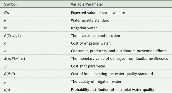
Less stringent irrigation water quality standard and greater use of irrigation water is assumed to increase social damages from contamination at an increasing rate, ${{\partial s} \over {\partial \theta }} \gt 0,\;\;{{\partial s} \over {\partial w}} \gt 0,\;\;{{{\partial ^2}S} \over {\partial {\theta ^2}}} \gt 0,{\rm{\;and\;}}{{{\partial ^2}S} \over {\partial {w^2}}} \gt 0.$
Damages are increasing in w because more irrigation implies greater potential contamination, foodborne illness and associated damages. An increase in preventative efforts of consumers and distributors is assumed to decrease marginal damages from additional water use,
${{\partial s} \over {\partial \theta }} \gt 0,\;\;{{\partial s} \over {\partial w}} \gt 0,\;\;{{{\partial ^2}S} \over {\partial {\theta ^2}}} \gt 0,{\rm{\;and\;}}{{{\partial ^2}S} \over {\partial {w^2}}} \gt 0.$
Damages are increasing in w because more irrigation implies greater potential contamination, foodborne illness and associated damages. An increase in preventative efforts of consumers and distributors is assumed to decrease marginal damages from additional water use, ${{{\partial ^2}S} \over {\partial \alpha \partial w}} \lt 0$
. Also,
${{{\partial ^2}S} \over {\partial \alpha \partial w}} \lt 0$
. Also, ${{{\partial ^2}S} \over {\partial w\partial \theta }} \gt 0$
, i.e., less stringent water quality standard leads to greater marginal damages from additional water use. Also,
${{{\partial ^2}S} \over {\partial w\partial \theta }} \gt 0$
, i.e., less stringent water quality standard leads to greater marginal damages from additional water use. Also, ${{\partial R} \over {\partial \theta }} \lt 0\;$
and
${{\partial R} \over {\partial \theta }} \lt 0\;$
and ${{{\partial ^2}R} \over {\partial {\theta ^2}}} \ge 0$
, i.e., costs of implementing the standard increase at an increasing rate. A decrease in the stringency of water quality standard is assumed to have a nonpositive effect on demand (i.e.,
${{{\partial ^2}R} \over {\partial {\theta ^2}}} \ge 0$
, i.e., costs of implementing the standard increase at an increasing rate. A decrease in the stringency of water quality standard is assumed to have a nonpositive effect on demand (i.e., ${{\partial P} \over {\partial \theta }} \le 0$
) with a decreasing rate (
${{\partial P} \over {\partial \theta }} \le 0$
) with a decreasing rate ( ${{{\partial ^2}P} \over {\partial {\theta ^2}}} \le 0$
). Increase in
${{{\partial ^2}P} \over {\partial {\theta ^2}}} \le 0$
). Increase in $\theta $
implies a less stringent standard, which is not likely to increase demand. The production function is assumed to be concave (i.e.,
$\theta $
implies a less stringent standard, which is not likely to increase demand. The production function is assumed to be concave (i.e., ${{\partial X} \over {\partial w}} \ge 0$
,
${{\partial X} \over {\partial w}} \ge 0$
, ${{{\partial ^2}X} \over {\partial {w^2}}} \lt 0$
). The first-order conditions with respect to
${{{\partial ^2}X} \over {\partial {w^2}}} \lt 0$
). The first-order conditions with respect to $\theta $
and w are
$\theta $
and w are
 $$\hskip-75pt{{\partial SW} \over {\partial \theta }} = \mathop \int \nolimits_0^X {{\partial P} \over {\partial \theta }}dX + {{\partial S} \over {\partial \theta }}\mathop \int \nolimits_z^\theta f\left( \mu \right)d\mu {\rm{\;}} - {\rm{\;}}{{\partial R} \over {\partial \theta }} = 0$$
 $${{\partial SW} \over {\partial w}} = P\left[ {X\left( w \right),\theta } \right]{{dX} \over {dw}}{\rm{\;}} - c - \mathop \int \nolimits_k^\theta {{\partial S} \over {\partial w}}f\left( \mu \right)d\mu + {{\partial S} \over {\partial w}}\mathop \int \nolimits_z^\theta f\left( \mu \right)d\mu = 0$$
Distribution of microbial water quality (top panel) and damages from foodborne illnesses (bottom panel).
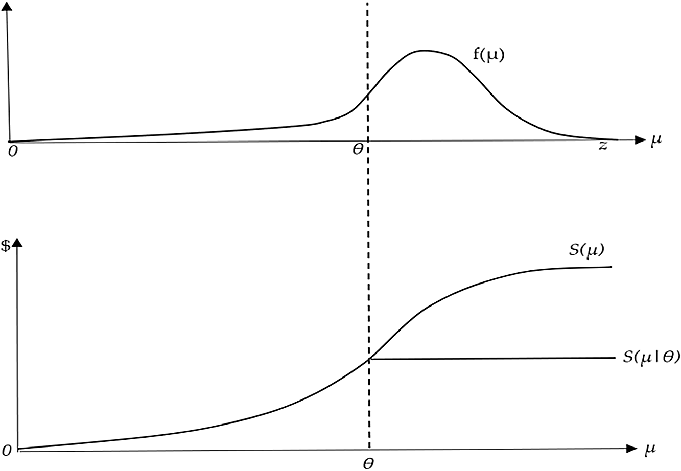
Propositions a, b, and c are obtained from the first-order conditions in equations (A.1) and (A.2) and the following second-order derivatives with respect to $\theta \;$
and w.
$\theta \;$
and w.
 $$\hskip-45pt{H_{11}} = {{{\partial ^2}SW} \over {\partial {\theta ^2}}} = \mathop \int \nolimits_0^X {{{\partial ^2}P} \over {\partial {\theta ^2}}}dX + {{{\partial ^2}S} \over {\partial {\theta ^2}}}\mathop \int \nolimits_z^\theta f\left( \mu \right)d\mu + {{\partial S} \over {\partial \theta }}f\left( \theta \right) - {{{\partial ^2}R} \over {\partial {\theta ^2}}} \le 0$$
 $${H_{22}} = {{{\partial ^2}SW} \over {\partial {w^2}}} = {{\partial P} \over {\partial X}}{\left( {{{dX} \over {dw}}} \right)^2} + P{{{d^2}X} \over {d{w^2}}} - \mathop \int \nolimits_0^\theta {{{\partial ^2}S} \over {\partial {w^2}}}f\left( \mu \right)d\mu + {{{\partial ^2}S} \over {\partial {w^2}}}\mathop \int \nolimits_z^\theta f\left( \mu \right)d\mu \le 0$$
 $$\hskip-80pt{H_{12}} = {\partial \over {\partial w}}\left( {{{\partial SW} \over {\partial \theta }}} \right) = {\partial \over {\partial w}}\left( {{{\partial S} \over {\partial \theta }}} \right)\mathop \int \nolimits_z^\theta f\left( \mu \right)d\mu + {{dX} \over {dw}}{{\partial P} \over {\partial \theta }} \le 0$$
 $${H_{21}} = {\partial \over {\partial \theta }}\left( {{{\partial SW} \over {\partial w}}} \right) = {\partial \over {\partial \theta }}\left( {{{\partial S} \over {\partial w}}} \right)\mathop \int \nolimits_z^\theta f\left( \mu \right)d\mu + {{dP} \over {d\theta }}{{dX} \over {dw}} \le 0$$
Comparative static results provide the following expressions for the impacts of the parameters of interest on the optimal water quality standard and optimal irrigation.
-
(1) The effect of water cost (c)
(A.7)
$$\left[ {\matrix{ {{H_{11}}} & {{H_{12}}} \cr {{H_{21}}} & {{H_{22}}} \cr } } \right]\left[ {\matrix{ {{{\partial \theta } \over {\partial c}}} \cr {{{\partial w} \over {\partial c}}} \cr } } \right] = \left[ {\matrix{ { - {\partial \over {\partial c}}\left( {{{\partial SW} \over {\partial \theta }}} \right)} \cr { - {\partial \over {\partial c}}\left( {{{\partial SW} \over {\partial w}}} \right)} \cr } } \right] = \left[ {\matrix{ 0 \cr 1 \cr } } \right]$$
(A.8)
$${{\partial \theta } \over {\partial c}} = {{\left| {\matrix{ 0 & {{H_{12}}} \cr 1 & {{H_{22}}} \cr } } \right|} \over {{H_{11}}{H_{22}} - {H_{12}}{H_{21}}}} = {{ - {H_{12}}} \over {{H_{11}}{H_{22}} - {H_{12}}{H_{21}}}} \ge 0$$
(A.9)
$${{\partial w} \over {\partial c}} = {{\left| {\matrix{ {{H_{11}}} & 0 \cr {{H_{21}}} & 1 \cr } } \right|} \over {{H_{11}}{H_{22}} - {H_{12}}{H_{21}}}} = {{{H_{11}}} \over {{H_{11}}{H_{22}} - {H_{12}}{H_{21}}}} \le 0$$
-
(2) The effect of cost of implementation of FSMA
$\left( \beta \right)$
(A.10)
$$\left[ {\matrix{ {{H_{11}}} & {{H_{12}}} \cr {{H_{21}}} & {{H_{22}}} \cr } } \right]\left[ {\matrix{ {{{\partial \theta } \over {\partial \beta }}} \cr {{{\partial w} \over {\partial \beta }}} \cr } } \right] = \left[ {\matrix{ { - {\partial \over {\partial \beta }}\left( {{{\partial SW} \over {\partial \theta }}} \right)} \cr { - {\partial \over {\partial \beta }}\left( {{{\partial SW} \over {\partial w}}} \right)} \cr } } \right] = \left[ {\matrix{ {{\partial \over {\partial \beta }}\left( {{{\partial R} \over {\partial \theta }}} \right)} \cr 0 \cr } } \right]$$
(A.11)
$${{\partial \theta } \over {\partial \beta }} = {{\left| {\matrix{ {{\partial \over {\partial \beta }}\left( {{{\partial R} \over {\partial \theta }}} \right)} & {{H_{12}}} \cr 0 & {{H_{22}}} \cr } } \right|} \over {{H_{11}}{H_{22}} - {H_{12}}{H_{21}}}} = {{{\partial \over {\partial \beta }}\left( {{{\partial R} \over {\partial \theta }}} \right){H_{22}}} \over {{H_{11}}{H_{22}} - {H_{12}}{H_{21}}}} \ge 0$$
(A.12)
$${{\partial w} \over {\partial \beta }} = {{\left| {\matrix{ {{H_{11}}} & {{\partial \over {\partial \beta }}\left( {{{\partial R} \over {\partial \theta }}} \right)} \cr {{H_{21}}} & 0 \cr } } \right|} \over {{H_{11}}{H_{22}} - {H_{12}}{H_{21}}}} = {{ - {\partial \over {\partial \beta }}\left( {{{\partial R} \over {\partial \theta }}} \right){H_{21}}} \over {{H_{11}}{H_{22}} - {H_{12}}{H_{21}}}} \le 0$$
-
(3) The effect of consumer and distributor efforts
$\left( \alpha \right)$
(A.13)
$$\left[ {\matrix{ {{H_{11}}} & {{H_{12}}} \cr {{H_{21}}} & {{H_{22}}} \cr } } \right]\left[ {\matrix{ {{{\partial \theta } \over {\partial \alpha }}} \cr {{{\partial W} \over {\partial \alpha }}} \cr } } \right] = \left[ {\matrix{ { - {\partial \over {\partial \alpha }}\left( {{{\partial SW} \over {\partial \theta }}} \right)} \cr { - {\partial \over {\partial \alpha }}\left( {{{\partial SW} \over {\partial w}}} \right)} \cr } } \right] = \left[ {\matrix{ {{\partial \over {\partial \alpha }}\left( {{{\partial S} \over {\partial \theta }}} \right)\mathop \int \nolimits_\theta ^z f\left( \mu \right)d\mu } \cr {\mathop \int \nolimits_0^\theta {\partial \over {\partial \alpha }}\left( {{{\partial S} \over {\partial w}}} \right)f\left( \mu \right)d\mu + {\partial \over {\partial \alpha }}\left( {{{\partial S} \over {\partial w}}} \right)\mathop \int \nolimits_\theta ^z f\left( \mu \right)d\mu } \cr } } \right]$$
(A.14)
$$\matrix{{{\partial \theta } \over {\partial \alpha }} = {{\left| {\matrix{ {{\partial \over {\partial \alpha }}\left( {{{\partial S} \over {\partial \theta }}} \right)\mathop \int \nolimits_\theta ^z f\left( \mu \right)d\mu } & {{H_{12}}} \cr {\mathop \int \nolimits_0^\theta {\partial \over {\partial \alpha }}\left( {{{\partial S} \over {\partial w}}} \right)f\left( \mu \right)d\mu + {\partial \over {\partial \alpha }}\left( {{{\partial S} \over {\partial w}}} \right)\mathop \int \nolimits_\theta ^z f\left( \mu \right)d\mu } & {{H_{22}}} \cr } } \right|} \over {{H_{11}}{H_{22}} - {H_{12}}{H_{21}}}} \hfill \cr \quad \;\; = {{{H_{22}}{\partial \over {\partial \alpha }}\left( {{{\partial S} \over {\partial \theta }}} \right)\mathop \int \nolimits_\theta ^z f\left( \mu \right)d\mu - {H_{12}}\left[ {\mathop \int \nolimits_0^\theta {\partial \over {\partial \alpha }}\left( {{{\partial S} \over {\partial w}}} \right)f\left( \mu \right)d\mu + {\partial \over {\partial \alpha }}\left( {{{\partial S} \over {\partial w}}} \right)\mathop \int \nolimits_\theta ^z f\left( \mu \right)d\mu } \right]} \over {{H_{11}}{H_{22}} - {H_{12}}{H_{21}}}} \hfill \cr }$$


Depending on the sign of ${S_{\alpha \theta }},\;$
the first term on the right-hand side in the numerator can be negative or positive while the second term is positive (assuming that
${S_{\alpha \theta }},\;$
the first term on the right-hand side in the numerator can be negative or positive while the second term is positive (assuming that ${\partial \over {\partial \alpha }}\left( {{{\partial SW} \over {\partial w}}} \right) \gt 0$
, i.e., an increase in consumer and distributor prevention efforts increases the marginal benefit of water use). This indicates that the impact of consumer and distributor effort on optimal water quality standard is positive or negative depending on the sign of
${\partial \over {\partial \alpha }}\left( {{{\partial SW} \over {\partial w}}} \right) \gt 0$
, i.e., an increase in consumer and distributor prevention efforts increases the marginal benefit of water use). This indicates that the impact of consumer and distributor effort on optimal water quality standard is positive or negative depending on the sign of ${S_{\alpha \theta }}$
.
${S_{\alpha \theta }}$
.
 $${{\partial \theta } \over {\partial \alpha }}\left\{ {\matrix{ { = ?\;\;\;\;\;,\;if\;\;{\partial \over {\partial \alpha }}\left( {{{\partial S} \over {\partial \theta }}} \right) \lt 0\;} \cr { \le 0\;\;\;\;,if\;\;{\partial \over {\partial \alpha }}\left( {{{\partial S} \over {\partial \theta }}} \right) \gt 0\;\;} \cr } } \right.$$
 $$\matrix{{{\partial w} \over {\partial \alpha }} = {{\left| {\matrix{ {{H_{11}}} & {{\partial \over {\partial \alpha }}\left( {{{\partial S} \over {\partial \theta }}} \right)\mathop \int \nolimits_\theta ^z f\left( \mu \right)d\mu } \cr {{H_{21}}} & {\mathop \int \nolimits_0^\theta {\partial \over {\partial \alpha }}\left( {{{\partial S} \over {\partial w}}} \right)f\left( \mu \right)d\mu + {\partial \over {\partial \alpha }}\left( {{{\partial S} \over {\partial w}}} \right)\mathop \int \nolimits_\theta ^z f\left( \mu \right)d\mu } \cr } } \right|} \over {{H_{11}}{H_{22}} - {H_{12}}{H_{21}}}} \hfill \cr \quad \;\; = {{\left[ {\mathop \int \nolimits_0^\theta {\partial \over {\partial \alpha }}\left( {{{\partial S} \over {\partial w}}} \right)f\left( \mu \right)d\mu + {\partial \over {\partial \alpha }}\left( {{{\partial S} \over {\partial w}}} \right)\mathop \int \nolimits_\theta ^z f\left( \mu \right)d\mu } \right]{H_{11}} - {H_{21}}{\partial \over {\partial \alpha }}\left( {{{\partial S} \over {\partial \theta }}} \right)\mathop \int \nolimits_\theta ^z f\left( \mu \right)d\mu } \over {{H_{11}}{H_{22}} - {H_{12}}{H_{21}}}}\hfill \cr }$$
Similarly, the first term on the right-hand side in the numerator is positive, while the second term can be positive or negative (depending on the sign of ${S_{\alpha \theta }}$
). This indicates that the sign of
${S_{\alpha \theta }}$
). This indicates that the sign of ${S_{\alpha \theta }}$
determines whether the impact of consumer and distributor effort on optimal water use is positive or negative.
${S_{\alpha \theta }}$
determines whether the impact of consumer and distributor effort on optimal water use is positive or negative.
 $${{\partial w} \over {\partial \alpha }}\left\{ {\matrix{ { = ?\;\;\;\;\;,\;if\;\;{\partial \over {\partial \alpha }}\left( {{{\partial S} \over {\partial \theta }}} \right) \lt 0\;} \cr { \ge 0\;\;\;\;,if\;\;{\partial \over {\partial \alpha }}\left( {{{\partial S} \over {\partial \theta }}} \right) \gt 0\;\;} \cr } } \right.$$
Appendix B Empirical model: demand response, FSMA cost, additional tables and figures
Demand response
Bovay and Sumner (Reference Bovay and Sumner2017) and Arnade et al. (Reference Arnade, Calvin and Kuchler2009) estimate that demand declines by 6.9% following an outbreak. This demand change corresponds to 204 cases of foodborne illnesses (Arnade et al. Reference Arnade, Calvin and Kuchler2009). We use these estimates to obtain the reduction in demand per case of foodborne illness (0.034%). Shuval et al. (Reference Shuval, Lampert and Fattal1997) estimate that the ratio of clinical illnesses caused by E. coli to the total number of infections is 1 to 100. Also, according to Scharff et al. (Reference Scharff, Besser, Sharp, Jones, Peter and Hedberg2016) and Scallan et al. (Reference Scallan, Griffin, Angulo, Tauxe and Hoekstra2011), only one in 26 symptomatic cases is reported in practice. We divide the demand shift parameter by 26*100 to obtain the demand response ( $\aleph $
) per reported clinical case, which is multiplied by the number of illnesses to obtain a demand response in each state of nature (
$\aleph $
) per reported clinical case, which is multiplied by the number of illnesses to obtain a demand response in each state of nature ( ${\varpi _n})$
(equation 18).
${\varpi _n})$
(equation 18).
FSMA costs
Cost of implementing FSMA is expressed as a downward sloping linear function of standard stringency ( $\theta $
). The intuition is that the implementation cost is greatest when
$\theta $
). The intuition is that the implementation cost is greatest when $\theta $
=0, which corresponds to the situation where any amount of E. coli results in producers having to take remediation measures. As the standard is relaxed (
$\theta $
=0, which corresponds to the situation where any amount of E. coli results in producers having to take remediation measures. As the standard is relaxed ( $\theta $
increases), the cost of implementing FSMA decreases.
$\theta $
increases), the cost of implementing FSMA decreases.
To obtain the values of slopes ( ${\xi _{f,GM}}{\rm{\;}}and$ ${\xi _{f,STV}}$
) and intercepts
${\xi _{f,STV}}$
) and intercepts $({M_{f,GM}}{\rm{\;}}and{\rm{\;}}{M_{f,STV}}),{\rm{\;}}$
we linearly approximate the implementation cost function between two points, A and B. We rely on FDA (2015b) to obtain costs of implementing FSMA, $27.5 and $21.1 million for small and large farms, respectively. We assume that these costs correspond to the water quality standard as proposed by the FDA (GM should not exceed 126 CFU per 100 ml of water and STV should not exceeds 410). This gives us point A. To linearly approximate the FSMA implementation cost function, we obtain the second point (B) using sufficiently high values of
$({M_{f,GM}}{\rm{\;}}and{\rm{\;}}{M_{f,STV}}),{\rm{\;}}$
we linearly approximate the implementation cost function between two points, A and B. We rely on FDA (2015b) to obtain costs of implementing FSMA, $27.5 and $21.1 million for small and large farms, respectively. We assume that these costs correspond to the water quality standard as proposed by the FDA (GM should not exceed 126 CFU per 100 ml of water and STV should not exceeds 410). This gives us point A. To linearly approximate the FSMA implementation cost function, we obtain the second point (B) using sufficiently high values of ${\rm{\;}}{\theta _{GM}}$
and
${\rm{\;}}{\theta _{GM}}$
and ${\theta _{STV}}$
(1,200 CFU/100 ml for GM and 3,900 CFU/100 ml for STV) so that FSMA regulatory constraint (equation 8) produces no delays in any state of nature across all random draws for irrigation water quality. In other words, smallest
${\theta _{STV}}$
(1,200 CFU/100 ml for GM and 3,900 CFU/100 ml for STV) so that FSMA regulatory constraint (equation 8) produces no delays in any state of nature across all random draws for irrigation water quality. In other words, smallest ${\rm{\;}}{\theta _{GM}}$
and
${\rm{\;}}{\theta _{GM}}$
and ${\theta _{STV}}$
values are identified such that equation (8) is never bunding across any state of nature. This corresponds to no FSMA regulation and no costs are incurred. This represents point B. We use these two points to derive a linear cost function for GM and STV. In the next step, we divide the intercepts and slopes by the acreages of farms as reported by the FDA (2015b) to obtain the per acre cost. Finally, we adjust these estimates by the percentages of lettuce acreage relative to total vegetable acreage from USDA (2017).
${\theta _{STV}}$
values are identified such that equation (8) is never bunding across any state of nature. This corresponds to no FSMA regulation and no costs are incurred. This represents point B. We use these two points to derive a linear cost function for GM and STV. In the next step, we divide the intercepts and slopes by the acreages of farms as reported by the FDA (2015b) to obtain the per acre cost. Finally, we adjust these estimates by the percentages of lettuce acreage relative to total vegetable acreage from USDA (2017).
Additional figures and tables
Summary of variables
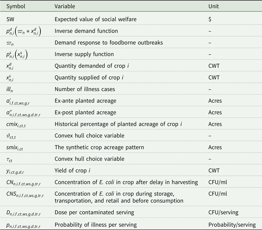
Summary of parameters
Own and cross elasticities of demand and own-price elasticity of supply of Head and Leaf-Romaine lettuce
Note: Own-price elasticities of demand are obtained from Okrent and Alston (Reference Okrent and Alston2012), cross-price elasticities of demand are derived from Ferrier et al. (Reference Ferrier, Zhen and Bovay2016), and own-price elasticities of supply are obtained from Lohr and Park (Reference Lohr and Park1992).
Comparison of simulation results and the observed data for Head and Leaf-Romaine lettuce
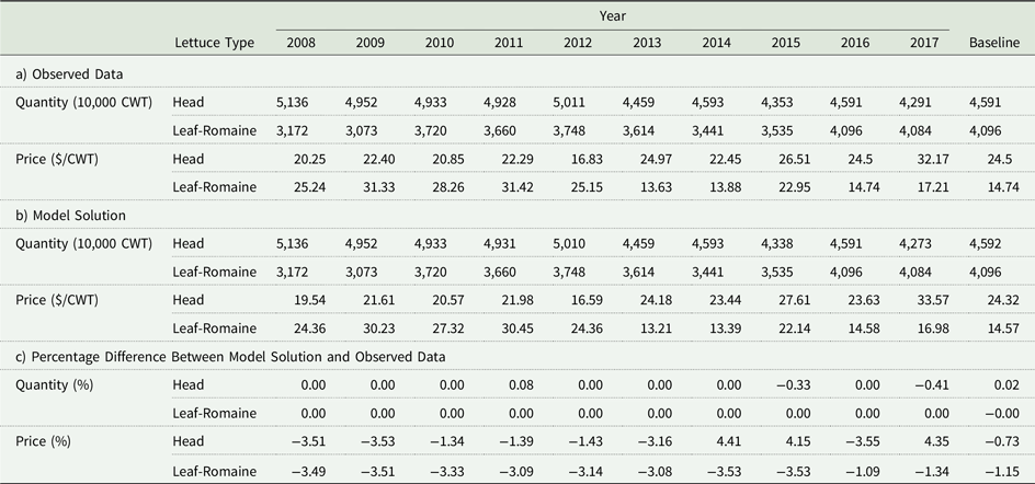
Average E. coli CFU per 100 ml of surface water and ground water in Arizona and California counties.
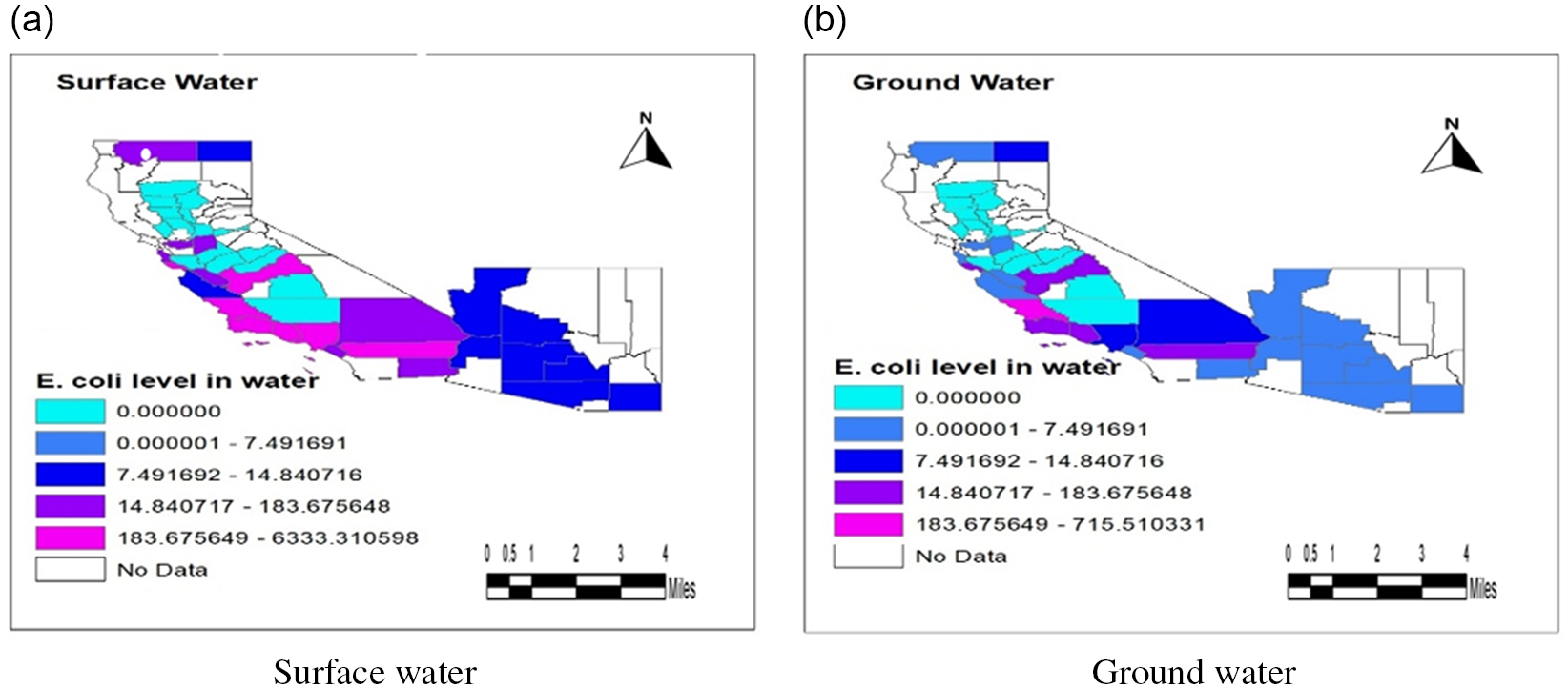


 Open access