

1. Introduction
1.1. Background
1.1.1. A little over a decade ago, the longevity risk transfer market started. This is now a global market, but it began in the UK in 2006. To coincide with the setup of this market, the British Actuarial Journal published Living with Mortality (Blake et al., Reference Blake, Cairns and Dowd2006a). That paper examined the problem of longevity risk – the risk surrounding uncertain aggregate mortality – and discussed the ways in which life insurers, annuity providers and pension plans could manage their exposure to this risk. In particular, it focused on how they could use mortality-linked securities and over-the-counter contracts – some existing and others still hypothetical – to manage their longevity risk exposures. It provided a detailed analysis of two such securities – the Swiss Re mortality bond issued in December 2003 and the European Investment Bank (EIB)/BNP Paribas longevity bond announced in November 2004. It then looked at the universe of hypothetical mortality-linked securities – other forms of longevity bonds, swaps, futures and options – and investigated their potential uses. It also addressed implementation issues and drew lessons from the experience with other derivative contracts. Particular attention was paid to the issues involved with the construction and use of mortality indices, the management of the associated credit risks and possible barriers to the development of markets for these securities. The paper concluded that these implementation difficulties were essentially teething problems that would be resolved over time, and so leave the way open to the development of a flourishing market in a brand new class of capital market securities.Footnote 1
1.1.2. In the event, the EIB/BNP longevity bond did not attract sufficient demand to get launched. The Swiss Re mortality bond, known as Vita,Footnote 2 was followed by broadly similar bonds from both Swiss Re and other issuers, but the overall size of the issuance was fairly small. Swiss Re also pioneered the successful issuance of a longevity-spread bond, known as Kortis,Footnote 3 but again the size of the issue was small. Investment banks, such as J. P. Morgan and Société Générale, introduced some innovative derivatives contracts – q-forwards and tail risk protection – but, so far, only a few of these contracts have been sold. Overall, then, the demand for the capital market solutions that have been proposed for hedging longevity risk has been disappointingly low.
1.1.3. By contrast, the solutions offered by the insurance industry have been much more successful. The key examples are the buy-out, the buy-in and longevity insurance. In other words, pension plan trustees, sponsors and advisers preferred dealing with risk by means of insurance contracts which fully removed the risk concerned and were not yet comfortable with capital market hedges that left some residual basis risk.
1.2. Focus of This Paper
The present paper provides a review of the developments in longevity risk management over the last decade or so. In particular, we focus on the ways in which pension plans and life insurers have managed their exposure to longevity risk, on why capital market securities failed to take off in the way that was anticipated 10 years ago, and what solutions for managing longevity risk might become available in the future.
1.3. Layout of This Paper
The paper is organised as follows. Section 2 quantifies the potential size of the longevity risk market globally. Section 3 discusses the different stakeholders in the market for longevity risk transfers. Sections 4 and 5, respectively, examine the structure of the successful insurance-based and capital market solutions that have been brought to market since 2006. The distinction between index and customised hedges and the issue of basis risk are investigated in section 6, while section 7 looks at credit risk, regulatory capital and collateral and section 8 discusses liquidity. Stochastic mortality models are crucial to the design and pricing of longevity risk transfer solutions and these are reviewed in section 9, while some applications that use these models are considered in section 10. Section 11 reviews the developments in the longevity de-risking market since 2006. Section 12 looks at potential future risk transfer solutions that involve the capital markets and section 13 concludes.
2. Quantifying the Potential Size of the Longevity Risk Market
2.1. Michaelson & Mulholland (Reference Michaelson and Mulholland2014) recently estimated the potential size of the global longevity risk market for pension liabilities at between $60trn and $80trn, comprising:
(i) The accumulated assets of private pension systems in the Organisation for Economic Co-Operation and Development (OECD) were $32.1trn,Footnote 4 arising from: pension funds (67.9%), banks and investment companies (18.5%), insurance companies (12.8%) and employers’ book reserves (0.8%) at year-end 2012 (OECD, 2013).
(ii) The US social security system had unfunded obligations for past and current participants of $24.3trn, as of the end of 2013 (Social Security Administration (SSA), 2013).
(iii) The aggregate liability of US State Retirement Systems was an additional $3trn, as of the end of 2012 (Morningstar, 2013), which does not capture the liabilities of countless US local and municipal pension systems.
(iv) There are public social security systems in 170 countries (excluding the USA) that provide old-age benefits of some sort for which reliable size estimates are not readily available but which are certainly substantial.Footnote 5
2.2. Michaelson & Mulholland (Reference Michaelson and Mulholland2014) then estimated the size of the longevity risk underlying these liabilities. Each additional year of unanticipated life expectancy at age 65 – roughly equivalent to a 0.8% increase in mortality improvements or a 13% reduction in mortality ratesFootnote 6 – can increase pension liabilities by 4–5%Footnote 7 (Swiss Re Europe, 2012). Risk Management Solutions (RMS) estimated the standard deviation of a sustained shock to annual mortality improvements (lasting 10 years or more) relative to expectations at around 0.80%. Michaelson and Mulholland use this estimate to calculate the effect of a longevity tail event (i.e. a 2.5 standard deviation event) which corresponds to a 2% change in trend (0.80%×2.5=2%) and, in turn, implies that longevity-related liabilities could increase by 10–12.5% as a result of unforeseen mortality improvements. Given aggregate global pension liabilities of $60–80trn, these could, in the extreme, turn out to be between $6trn and 10trn higher.
2.3. Pigott & Walker (Reference Pigott and Walker2016) also estimate that private sector longevity risk exposure is of the order of $30trn.Footnote 8 This is concentrated in the US ($14.460trn), the UK ($2.685trn), Australia ($1.639trn), Canada ($1.298trn), Holland ($1.282trn), Japan ($1.221trn), Switzerland ($0.788trn), South Africa ($0.306trn), France ($0.272trn), South America ($0.251trn), Germany ($0.236trn) and Hong Kong ($0.110trn). Pigott and Walker argue that only the UK, USA, Canada and Holland currently have the conditions for a longevity risk transfer market to develop. These conditions include: low interest rates (in part due to government quantitative easing programmes in response to the 2007–2008 Global Financial Crisis (GFC)) which, by increasing the present value of more distant pension payments, has exposed the real extent of longevity risk in pension plans; inflation uplifting of pensions in payment further increases longevity risk; frequent updating by the actuarial profession of longevity projections; the introduction of market-consistent valuation methods; increased accounting transparency of pension assets and liabilities; and increased intervention powers by the regulator. Collectively, these factors have focussed the minds of plan trustees and sponsors and encouraged them to look for solutions with their advisers.
2.4. The other markets do not currently have the right conditions for the following reasons:
∙ Australia: Most sponsors of pension plans bear little or no longevity risk; individuals often take a lump sum or buy term (20-year) annuities at retirement, then rely on the state, although a lifetime annuity market is beginning to emerge.
∙ Japan: Corporate sponsors of pension plans and insurers do not bear longevity risk, since individuals buy term annuities at retirement; however, there is a growing market for long-term annuities in Japan purchased from Australia.Footnote 9
∙ Switzerland: Individuals are incentivised but not required to annuitise; the market is small, but may open up in the future.
∙ Germany: Occupational plan liabilities are often written onto company balance sheets as book reserves, so there is little resource or incentive to de-risk, despite longevity risk being as significant a risk as it is in other countries.
∙ France: A very small market, although French insurers and reinsurers are active in other markets.
∙ South Africa and South America: Hampered by lack of or unreliable historical mortality data and poor experience data; in Chile, which has a rapidly growing lifetime annuities market, the government effectively underwrites annuity providers which therefore have no incentive to hedge their longevity risk exposure.Footnote 10
3. Stakeholders in the Longevity Risk Transfer Market
3.1. Classes of Stakeholders
Figure 1 shows the participants in the longevity risk transfer market. In this section, we examine the various classes of stakeholders in this market.
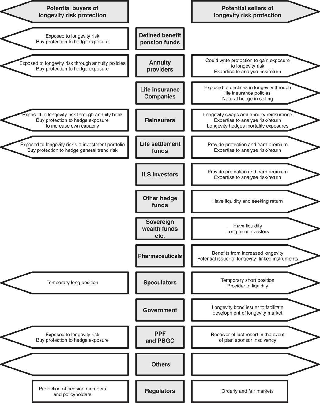
Figure 1 Participants in the Longevity Risk Transfer Market
Source: Adapted from Loeys et al. (Reference Loeys, Panigirtzoglou and Ribeiro2007, Chart 10); PPF, Pension Protection Fund, PBGC, Pension Benefit Guaranty Corporation.
3.2. Hedgers
3.2.1. One natural class of stakeholders are hedgers, those who have a particular exposure to longevity risk and wish to lay off that risk. For example, defined benefit (DB) pension funds and annuity providers stand to lose if mortality improves by more than anticipated, while life insurance companies stand to gain, and vice versa. These offsetting exposures imply that annuity providers and life assurers, for example, can hedge each other’s longevity risks.Footnote 11 Alternatively, parties with unwanted exposure to longevity risk might pay other parties to lay off some of their risk. For instance, a life office might hedge its longevity risk using a reinsurer or by selling it to capital market institutions.
3.2.2. As another possibility, pharmaceutical companies benefit if people live longer, since they (and the health service) need to spend more on medicines as they get older, especially for those in poor health. Also there is a continuous stream of new medical treatments that prolong life. The pharmaceutical companies could potentially issue longevity-linked debt to finance their research and development programmes which, if sufficiently attractive for pension funds to hold, could be issued at a lower cost than conventional fixed maturity debt. In other words, pharmaceutical companies benefit if longevity increases and could put on a counterbalancing position by issuing longevity bonds.Footnote 12 While they have been approached about this possibility, no pharmaceutical company has yet issued such debt. The principal reasons appear to be that the finance directors have not been made sufficiently aware of the potential benefits of such an issue – and in any case are more concerned that the millions of dollars being spent on drug trials will bring a sufficient return to shareholders – and because, in practice, the short-term correlation between company profits and longevity is probably not strong enough to persuade finance directors to issue longevity bonds.
3.3. Specialist and General Investors
There are specialist investors in this market, such as life settlementFootnote 13 investors, premium finance investors,Footnote 14 and insurance-linked securities (ILS) investors.Footnote 15 Depending on their existing exposures, these investors could either buy longevity protection or sell it and earn a premium. General investors include short-term investors, such as hedge funds and private equity investors and long-term investors, such as sovereign wealth funds, endowments and family offices. Provided expected returns are acceptable, such investors might be interested in acquiring an exposure to longevity risk, since it has a low correlation with standard financial market risk factors. The combination of a low beta and a potentially positive alpha should therefore make mortality-linked securities attractive investments in diversified portfolios.
3.4. Speculators and Arbitrageurs
A market in longevity-linked securities might attract speculators: short-term investors who trade their views on the direction of individual security price movements. The active involvement of speculators is important for creating market liquidity as a by-product of their trading activities, and is in fact essential to the success of traded futures and options markets. However, liquidity also depends on the frequency with which new information about the market materialises and this is currently sufficiently low that there is negligible speculator interest in the longevity market at the present time. Arbitrageurs seek to profit from any pricing anomalies in related securities. For arbitrage to be a successful activity, it is essential that there are well-established pricing relationships between the related securities: periodically, prices get out of line which creates profit opportunities which arbitrageurs exploit.Footnote 16 However, the longevity market is currently not sufficiently well developed for arbitrage opportunities to exist.
3.5. Governments
3.5.1. Governments have many potential reasons to be interested in markets for longevity-linked securities. They might wish to promote such markets and assist financial institutions that are exposed to longevity risk (e.g. they might issue longevity bonds that can be used as instruments to hedge longevity risk).Footnote 17
3.5.2. Governments might also be interested in managing their own exposure to longevity risk. They are a significant holder of this risk in their own right via pay-as-you-go state pensions, pensions to former public sector employees and their obligations to provide health care for the elderly. At a higher level, governments are affected by numerous other economic factors, some of which partially offset their own exposure to longevity risk (for example income tax on private pensions continues to be paid as people live longer).
3.6. Regulators
3.6.1. Financial regulators have two main stated aims: (i) the enhancement of financial stability through the promotion of efficient, orderly and fair markets and (ii) ensuring that retail customers get a fair deal.Footnote 18 The two financial regulators in the UK responsible for delivering on these aims are the Prudential Regulatory Authority (PRA) and the Financial Conduct Authority (FCA).
3.6.2. The PRA has a duty to ensure that the financial system is protected against systemic risks and longevity risk is a potential example of such a risk. This, in turn, requires that carriers of such risks, such as life insurance companies, issue sufficient regulatory capital to protect themselves from insolvency with a high degree of probability. The FCA’s duty is to ensure that customers get competitive and fairly priced annuity products, for example, and that becomes more difficult if providers of these products cannot easily or economically hedge the longevity risk contained in them.Footnote 19
3.6.3. Another interested regulator is The Pensions Regulator (TPR) which acts as gatekeeper to the UK’s pension lifeboat, the Pension Protection Fund (PPF).Footnote 20 TPR wants to reduce the probability that large companies (in particular) are bankrupted by their pension funds (Harrison & Blake, Reference Harrison and Blake2016). As “insurer of last resort,” the Government is also potentially the residual holder of this risk in the event of default by the PPF. The PPF and Government have a strong incentive to help companies hedge their exposure to longevity risk, which would reduce the likelihood of claims on the PPF. The PPF faces the systematic risk that longevity projections go up generally for plans (without diversifying away between plans), which (i) pushes some plans into the PPF and (ii) increases existing PPF liabilities.Footnote 21
3.7. Other Stakeholders
Other domestic stakeholders include healthcare providers and insurers, providers of equity release (or reverse or lifetime) mortgages and securities managers and organised exchanges, all of which would benefit from a new source of fee income. Members of both DB and defined contribution (DC) plans have an interest in protecting their current and future pension entitlements, although the risks in the two types of plan are different. In the case of DB, the security of the plan itself is at stake, with the member facing the risk of lower (e.g. PPF) benefits if the plan sponsor becomes insolvent. In the case of DC, the member is exposed either to the vagaries of the individual annuities market or to the risk of drawing down benefits too quickly and surviving longer than expected. Finally, individuals with state pensions are ultimately not immune from increases in the government’s budget deficit that arise from increases in life expectancy: (i) state pensions could fall (in real terms) for current pensioners, (ii) the state pension age could increase even further than currently planned for future pensioners and (iii) all current and future generations of tax payers are ultimately liable for the increased cost. Longevity risk is a global phenomenon, so there will be similar stakeholders in other countries where this problem is prevalent.
4. Successful Insurance-Based Solutions
4.1. Overview
The traditional solution for dealing with unwanted longevity risk in a DB pension plan or an annuity book is to sell the liability via an insurance or reinsurance contract. This is known as a pension buy-out (or pension termination) or, in an insurance context, a group/bulk annuity transfer. More recently, pension buy-ins and longevity insurance (the insurance term for a longevity swap) have been added to the list of insurance-based solutions for transferring longevity risk. Insurance solutions are generally classified as “customised indemnification solutions,” since the insurer fully indemnifies the hedger against its specific risk exposure. These solutions can also be thought of as “at-the-money” hedges, since the hedge provider is responsible for any increase in the liability above the current best estimate assumption on a pound-for-pound basis.
4.2. Pension Buy-outs
4.2.1. The most common traditional solution for DB pension plans is a full pension buy-out, implemented by a regulated life assurer. The procedure can be illustrated using the following simple example.
4.2.2. Consider Company ABC with pension plan assets (A) of 85 and pension plan liabilities (L) of 100, valued on an “ongoing basis”Footnote 22 by the plan actuary; this implies a deficit of 15. ABC approaches life assurer XYZ to effect a pension buy-out. On a full “buy-out basis,” the insurer values the pension liabilities at 120, a premium of 20 to the plan actuary’s valuation, implying a buy-out deficit of 35. The insurer, subject to due diligence, offers to take on both the plan assets A and plan liabilities L provided the company contributes 35 from its own resources (or from borrowing) to cover the buy-out deficit. Following the acquisition, the insurer implements an asset transition plan which involves exchanging certain assets, e.g. cash or equities for bonds or loans, and implementing interest rate and inflation swaps to hedge the interest-rate and inflation risk associated with the pension liabilities.Footnote 23
4.2.3. The advantages to the company are that the pension liabilities are completely removed from its balance sheet. In the case where the company does not have the cash resources to pay the full cost of the buy-out, the pension deficit (on a buy-out basis) is often replaced by a loan which, unlike fluctuating pension liabilities, is an obligation that is readily understood by investment analysts and shareholders. The company avoids volatility in its profit and loss account coming from the pension plan,Footnote 24 the payment of levies to the PPF, administration fees on the plan and the potential drag on its enterprise value arising from the pension plan. The advantage of a buy-out to the pension trustees and plan members is that pensions are now secured in full (subject to the credit risk of the life assurer).
4.2.4. There is a potential disadvantage in terms of timing. Once a buy-out has taken place, it cannot generally be renegotiated if circumstances change and the buy-out price is lower in the future, say, because an increase in long-term interest rates leads to the discount rate used to value pension liabilities also increasing. There is also a potential risk that the buy-out company itself becomes insolvent in which case the pensioners would have no recourse to the PPF. However, since buy-out companies are established as insurance companies with solvency capital requirements,Footnote 25 this risk should, in practice, be very low in countries like the UK.
4.3. Pension Buy-ins
4.3.1. Buy-ins are insurance transactions that involve the bulk purchase of annuities by the pension plan to hedge the risks associated with a subset of the plan’s liabilities, typically associated with retired members. The annuities become an asset of the plan and cover the specific mortality characteristics of the plan’s membership in terms of age, gender and pension amount – but the individual members do not receive annuity certificates.
4.3.2. Buy-ins are often part of the journey to a full buy-out. They can be thought of as providing a “de-risking” of the pension plan in economic terms. If purchased in phases, they enable the plan to smooth out annuity rates over time and avoid a spike in pricing at the time it decides to proceed directly to a full buy-out. Buy-ins also offer the sponsor the advantage of full immunisation of a portion of the pension liabilities for a lower up-front cash payment relative to a full buy-out – although the recent introduction of deferred premium payments for both buy-ins and buy-outs has helped to spread costs for both types of product.Footnote 26
4.3.3. Since the annuity contract purchased in a buy-in is an asset of the pension plan, rather than an asset of the plan member, the pension liability remains on the balance sheet of the sponsor. Plan members are therefore still exposed to the risk of sponsor insolvency if the plan is in deficit and (indirectly) to the risk of insurance company insolvency unless the buy-in deal has been fully collateralised.
4.4. Longevity Insurance or Insurance-Based Longevity Swaps
4.4.1. The third successful solution is the longevity insurance contract or insurance-based longevity swap. This is effectively an insurance version of the capital-markets-based longevity swap (discussed in the next section), which transfers longevity risk only.Footnote 27 A typical structure involves the buyer of the swap paying a pre-agreed fixed set of cash flows to the swap provider and receiving in exchange a floating set of cash flows linked to the realised mortality experience of the swap buyer, the latter being used to pay the pensions for which the swap buyer is liable. No assets are transferred and the pension plan typically retains the investment risks associated with the asset portfolio. Longevity swaps have the advantage that they remove longevity risk without the need for an upfront payment by the sponsor and allow the pension plan trustees to retain control of the asset allocation.
4.4.2. The first publicly announced longevity swap took place in April 2007 between Swiss Re and Friends’ Provident, a UK life insurer. It was a pure longevity risk transfer and was not tied to another financial instrument or transaction. The swap was based on Friends’ Provident’s £1.7bn book of 78,000 pension annuity contracts written between July 2001 and December 2006. Friends’ Provident retains administration of policies. Swiss Re makes payments and assumes longevity risk in exchange for an undisclosed premium.
4.4.3. In any longevity swap, the hedger of longevity risk (e.g. a pension plan or insurer) receives from the longevity swap provider the actual paymentsFootnote 28 it must pay to pensioners and, in return, makes a series of fixed payments to the hedge provider.Footnote 29 In this way, if pensioners live longer than expected, the higher pension amounts that the pension plan must pay are offset by the higher payments received from the provider of the longevity swap. The swap therefore provides the pension plan with a long-maturity, customised cash flow hedge of its longevity risk.
4.4.4. Figure 2 shows the set of cash flows in a typical longevity swap involving a pension plan wishing to hedge its longevity risk exposure. The plan makes a set of pre-agreed fixed payments (each payment is based on an amount-weighted survival rate (Dowd et al., Reference Dowd, Blake, Cairns and Dawson2006; Dawson et al., Reference Dawson, Blake, Cairns and Dowd2010)) and receives the actual pension payments it needs to make (these will be based on its realised longevity experience).

Figure 2 A longevity swap involves the regular exchange of actual realised pension cash flows and pre-agreed fixed cash flows
Source: Coughlan (Reference Coughlan2007a).
5. Successful Capital Markets Solutions
5.1. Overview
In this section, we analyse the small number of capital market securities that have been successfully launched since 2006: longevity-spread bonds, longevity swaps, q-forwards, S-forwards and tail-risk protection (or longevity bull call spreads). The key feature of these is that most are index rather than customised solutions.Footnote 30
5.2. Longevity-Spread Bonds
5.2.1. In December 2010, Swiss Re issued an 8-year catastrophe-type bond linked to longevity spreads. To do this, it used a special purpose vehicle, Kortis Capital, based in the Cayman Islands.Footnote 31 The Kortis bond is designed to hedge Swiss Re’s own exposure to longevity risk.Footnote 32 It had a very small nominal value of just $50 m, which clearly meant that it was designed to test the water for a new type of capital market instrument.
5.2.2. The bond holders received quarterly coupons equal to 3-month LIBOR plus a margin. In exchange, they were exposed to the risk that the difference between the annualised mortality improvement in English & Welsh males aged 75–85 over a period of 8 years and the corresponding improvement in US males aged 55–65 is significantly larger than anticipated. The mortality improvements were measured over 8 years from 1 January 2009 to 31 December 2016. The bonds matured on 15 January 2017,Footnote 33 although there was an option to extend the maturity to 15 July 2019. The principal was at risk if the Longevity Divergence Index Value (LDIV) exceeded the attachment point or trigger level of 3.4% over the risk period. The exhaustion point, at or above which there would be no return of principal, is 3.9%. The principal would be reduced by the principal reduction factor (PRF) if the LDIV lies between 3.4% and 3.9%.
5.2.3. The LDIV is derived as follows. Let m y (x,t) be the male death rate at age x and year t in country y. This is defined as the ratio of deaths to population size for the relevant age and year. Annualised mortality improvements over n years are defined as:
 $$Improvement_{n}^{y} \left( {x,t} \right){\equals}1{\minus}\left[ {{{m^{y} \left( {x,t} \right)} \over {m^{y} \left( {x,t{\minus}n} \right)}}} \right]^{{{1 \over n}}} $$
The annualised mortality improvement index for each age group is found by averaging the annualised mortality improvements across ages x 1 to x 2 in the group:
 $$Index\left( y \right){\equals}{1 \over {1{\plus}x_{2} {\minus}x_{1} }}\mathop{\sum}\limits_{x{\equals}x_{1} }^{x{\equals}x_{2} } {Improvement_{n}^{y} \left( {x,t} \right)} $$
In the case of the Kortis bond, n is equal to 8 years. The LDIV is defined as:
 $$LDIV{\equals}Index\left( {y_{2} } \right){\minus}Index\left( {y_{1} } \right)$$
where y 2 is the England & Wales population aged 75–85 and y 1 is the US population aged 55–65. The PRF is calculated as follows:
 $$PRF{\equals}{{LDIV{\minus}Attachment\,point} \over {Exhaustion\,point{\minus}Attachment\,point}}$$
with a minimum of 0% and a maximum of 100%.
5.2.4. Proceeds from the sale of the bond were deposited in a collateral account at the AAA-rated International Bank for Reconstruction and Development (i.e. the World Bank). If there is a larger-than-expected difference between the mortality improvements of 75–85 year old English & Welsh males and those of 55–65 year old US males, part of the collateral will be sold to make payment to Swiss Re and, as a consequence, the principal of the bond would be reduced. The exposure that Swiss Re wished to hedge comes from two different sources. For example, Swiss Re is the counterparty in a £750 m longevity swap with the Royal County of Berkshire Pension Fund which was executed in 2009, and so is exposed to high-age English & Welsh males living longer than anticipated. It has also reinsured a lot of US life insurance policies and is exposed to middle-aged US males dying sooner than expected. The longevity-spread bond provided a partial hedge for both tail exposures.
5.2.5. Standard & Poor’s rated the bond BB+ which took into account the possibility that investors would not receive the full return of their principal. This rating was determined using two models developed by RMS which was appointed as the calculation agent for the bonds.Footnote 34
5.2.6. Table 1 shows estimated loss probabilities for the bond using the RMS models. Figure 3 presents a fan chart of the projected LDIV showing the 98% confidence interval.
Table 1 Estimated Loss Probabilities for the Swiss Re Longevity-Spread Bond

Note: (1)attachment probability; (2)exhaustion probability.
Source: Standard and Poor’s (2010) Presale information: Kortis Capital Ltd. Tech. Report.

Figure 3 Fan chart of the projected LDIV showing the 98% confidence interval
Source: Hunt & Blake (Reference Hunt and Blake2015, Figure 8).
5.2.7. This was the first time that the risk of individuals living longer than expected has been traded in the form of a bond. Investors had been reluctant to hold longevity risk long term, but short-term bonds might make bearing the risk more acceptable. The bond therefore represented a significant breakthrough for capital market solutions. Nevertheless, there appears to have been very little trading in the bond and no further examples of the bond have so far been issued.
5.3. Capital-Markets-Based Longevity Swaps
5.3.1. The first capital-markets-based longevity swap took place in July 2008 between J. P. Morgan and Canada Life in the UK (Trading Risk, 2008). The contract was a 40-year maturity £500 m longevity swap that was linked to the actual mortality experience of the 125,000-plus annuitants in the annuity portfolio that was being hedged. This transaction brought capital markets investors into the longevity market for the very first time, as the longevity risk was passed from Canada Life to J. P. Morgan and then directly on to investors.
5.3.2. This has become the archetypal longevity swap upon which other transactions are based. Insurance companies, such as Rothesay Life, have adapted its structure and collateralisation terms to an insurance format.
5.3.3. It is important to note that the J. P. Morgan – Canada Life swap was a customised swap, since it was linked to the actual mortality experience of the hedger. All insurance-based longevity swaps in the UK have also been customised swaps to date. However, such swaps are harder to priceFootnote 35 and are potentially more illiquid than index-based swaps which are based on the mortality experience of a reference population, such as the national population. Most longevity swaps sold into the capital markets are index-based. These issues are discussed in more detail in section 8.
5.4. q-Forwards (or Mortality Forwards) and S-Forwards (or Survivor Forwards)
5.4.1. A mortality forward rate contract is referred to as a “q-forward” because the letter “q” is the standard actuarial symbol for a mortality rate. It is the simplest type of instrument for hedging longevity (and mortality) risk (Coughlan et al., Reference Coughlan, Epstein, Sinha and Honig2007b).Footnote 36 , Footnote 37
5.4.2. The first capital markets transaction involving a q-forward took place in January 2008. The hedger was buy-out company Lucida (Lucida, 2008; Symmons, Reference Symmons2008). The q-forward was linked to a longevity index based on England & Wales national male mortality for a range of different ages. The hedge was provided by J. P. Morgan and was novel not just because it involved a longevity index and a new kind of product, but also because it was designed as a hedge of value rather than a hedge of cash flow. In other words, it hedged the value of an annuity liability,Footnote 38 not the actual individual annuity payments.
5.4.3. Formally, a q-forward is a contract between two parties in which they agree to exchange an amount proportional to the actual realised mortality rate of a given population (or sub-population), in return for an amount proportional to a fixed mortality rate that has been mutually agreed at inception to be payable at a future date (the maturity of the contract). In this sense, a q-forward is a swap that exchanges fixed mortality for the realised mortality at maturity, as illustrated in Figure 4. The variable used to settle the contract is the realised mortality rate for that population in a future period. In the case of hedging longevity risk in a pension plan using a q-forward, the plan will receive the fixed mortality rate and pay the realised mortality rate (and hence, over the term of the contract, locks in the future mortality rate it has to pay whatever happens to actual rates). The counterparty to this transaction, typically an investment bank, has the opposite exposure, paying the fixed mortality rate and receiving the realised rate.
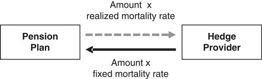
Figure 4 A q-forward exchanges fixed mortality for realised mortality at the maturity of the contract
Source: Coughlan et al. (Reference Coughlan, Epstein, Sinha and Honig2007b, Figure 1)
5.4.4. The fixed mortality rate at which the transaction takes place defines the “forward mortality rate” for the population in question. If the q-forward is fairly priced, no payment changes hands at the inception of the trade, but at maturity, a net payment will be made by one of the two parties (unless the fixed and actual mortality rates happen to be the same). The settlement that takes place at maturity is based on the net amount payable and is proportional to the difference between the fixed mortality rate (the transacted forward rate) and the realised reference rate. If the reference rate in the reference year is below the fixed rate (implying lower mortality than predicted), then the settlement is positive, and the pension plan receives the settlement payment to offset the increase in its liability value. If, on the other hand, the reference rate is above the fixed rate (implying higher mortality than predicted), then the settlement is negative and the pension plan makes the settlement payment to the hedge provider, which will be offset by the fall in the value of its liabilities. In this way, the net liability value is hedgedFootnote 39 regardless of what happens to mortality rates. The plan is protected from unexpected changes in mortality rates.
5.4.5. Table 2 presents an illustrative term sheet for a q-forward transaction, based on a reference population of 65-year-old males from England & Wales. The q-forward payout depends on the value of the LifeMetrics Index for the reference population on the maturity date of the contract. The particular transaction shown is a 10-year q-forward contract starting on 31 December 2008 and maturing on 31 December 2018. It is being used by ABC Pension Fund to hedge its longevity risk over this period; the hedge provider is J. P. Morgan. The hedge is a “directional hedge” and will help the pension fund hedge its longevity risk so long as the mortality experience of the pension fund and the index change in the same direction.
Table 2 An Illustrative Term Sheet for a Single q-forward to Hedge Longevity Risk

Source: Coughlan et al. (Reference Coughlan, Epstein, Sinha and Honig2007b, Table 1).
5.4.6. On the maturity date, J. P. Morgan (the fixed-rate payer or seller of longevity risk protection) pays ABC Pension Fund (the floating-rate payer or buyer of longevity risk protection) an amount related to the pre-agreed fixed mortality rate of 1.2000% (i.e. the agreed forward mortality rate for 65-year-old English & Welsh males for 2018). In return, ABC Pension Fund pays J. P. Morgan an amount related to the reference rate on the maturity date. The reference rate is the most recently available value of the LifeMetrics Index. Settlement on 31 December 2018 will therefore be based on the LifeMetrics Index value for the reference year 2017, on account of the 10-month lag in the availability of official data. The settlement amount is the difference between the fixed amount (which depends on the agreed forward rate) and the floating amount (which depends on the realised reference rate).
5.4.7. Table 3 shows the settlement amounts for four realised values of the reference rate and a notional contract size of £50 m. If the reference rate in 2017 is lower than the fixed rate (implying lower mortality than anticipated at the start of the contract), the settlement amount is positive and ABC Pension Fund receives a payment from J. P. Morgan that it can use to offset an increase in its pension liabilities. If the reference rate exceeds the fixed rate (implying higher mortality than anticipated at the start of the contract), the settlement amount is negative and ABC Pension Fund makes a payment to J. P. Morgan which will be offset by a fall in its pension liabilities.
Table 3 An Illustration of q-Forward Settlement for Various Outcomes of the Realised Reference Rate

Source: Coughlan et al. (Reference Coughlan, Epstein, Sinha and Honig2007b, Table 1): A positive (negative) settlement means the hedger pays (receives) the net settlement amount.
5.4.8. It is important to note that the hedge illustrated here is structured as a “value hedge,” rather than as a “cash flow hedge.” A value hedge aims to hedge the value of the hedger’s liabilities at the maturity date of the swap. So although the swap has a duration of only 10 years, it nevertheless hedges that portion of the longevity risk in the hedger’s cash flows beyond 10 years that are reflected in mortality rates at time 10. This is achieved by exchanging a single payment at maturity. By contrast, a cash flow hedge hedges the longevity risk in each one of the hedger’s cash flows and net payments are made period by period as in Figure 2. The J. P. Morgan-Canada Life longevity swap is an example of a cash flow hedge, while the J. P. Morgan-Lucida q-forward is an example of a value hedge. The capital markets are more familiar with value hedges, whereas cash flow hedges are more common in the insurance world. Value hedges are particularly suited to hedging the longevity risk of younger members of a pension plan, since it is much harder to estimate with precision the pension payments they will receive when they eventually retire. The world’s first swap for non-pensioners (i.e. involving deferred members) took place in January 2011 when J. P. Morgan executed a value hedge in the form of a 10-year q-forward contract with the Pall (UK) pension fund.
5.4.9. The importance of q-forwards rests in the fact that they form basic building blocks from which other more complex, life-related derivatives can be constructed. When appropriately designed, a portfolio of q-forwards can be used to replicate and to hedge the longevity exposure of an annuity or a pension liability, or to hedge the mortality exposure of a life assurance book. We now provide an example.
5.4.10. A series of q-forward contracts, with different ages and maturities, can be combined to hedge a longevity swap. Initially assume that there is a complete market in these contracts for all ages and maturities. Suppose the contract involves swapping at time t a fixed cashflow, $\tilde{S}(t)$
, for the realised survivor index, S(t,x), where x is the age of the group being hedged at the inception of the swap. The fixed leg can be hedged using zero-coupon fixed-income bonds. The floating leg can be hedged approximately as follows. First, note that we can approximate the survivor index by expanding the cashflow in terms of the fixed legs of a set of q-forwards and their ultimate net payoffs (see Cairns et al., Reference Cairns, Blake and Dowd2008):
$\tilde{S}(t)$
, for the realised survivor index, S(t,x), where x is the age of the group being hedged at the inception of the swap. The fixed leg can be hedged using zero-coupon fixed-income bonds. The floating leg can be hedged approximately as follows. First, note that we can approximate the survivor index by expanding the cashflow in terms of the fixed legs of a set of q-forwards and their ultimate net payoffs (see Cairns et al., Reference Cairns, Blake and Dowd2008):
 $$\eqalignno{ & S\left( {t,x} \right){\equals}\left( {1{\minus}q\left( {0,x} \right)} \right){\times}\left( {1{\minus}q\left( {1,x{\plus}1} \right)} \right){\times}...{\times}\left( {1{\minus}q\left( {t{\minus}1,x{\plus}t{\minus}1} \right)} \right) \cr & \,\,\,\,\,\,\,\,\,\,\,\,\,\,\,{\equals}\prod\limits_{i{\equals}0}^{t{\minus}1} {\left( {1{\minus}q_{F} \left( {0,i,x{\plus}i} \right){\minus}\Delta \left( {i,x{\plus}i} \right)} \right)} \cr & \,\,\,\,\,\,\,\,\,\,\,\,\,\,\,\,\approx\,\prod\limits_{i{\equals}0}^{t{\minus}1} {\left( {1{\minus}q_{F} \left( {0,i,x{\plus}i} \right)} \right)} \cr & \,\,\,\,\,\,\,\,\,\,\,\,\,\,\,\,\,\,\,\,\,\,\,\,\,\,\,\,{\minus}\mathop{\sum}\limits_{i{\equals}0}^{t{\minus}1} {\Delta \left( {i,x{\plus}i} \right)} \prod\limits_{j{\equals}0,j\,\ne\,i}^{t{\minus}1} {\left( {1{\minus}q_{F} \left( {0,j,x{\plus}j} \right)} \right)} $$
where Δ(i, x + i)=q(i, x + i)−q F (0, i, x + i) and q F (0, i, x + i)=q-forward mortality rate (the fixed rate). Here, Δ(i, x + i) is the net payoff on the q-forward per unit at time i + 1.
5.4.11. It follows that an approximate hedge (assuming interest rates are constant and equal to r per annum) for S(t, x) can be achieved by holding:
∙
 $${\minus}\left( {1{\plus}r} \right)^{{{\minus}(t{\minus}1)}} \prod\nolimits_{j{\equals}0,\,j\,\ne\,1}^{t{\minus}1} {\left( {1{\minus}q_{F} \left( {0,j,x{\plus}j} \right)} \right)} $$
units of the 1-year q-forward;
$${\minus}\left( {1{\plus}r} \right)^{{{\minus}(t{\minus}1)}} \prod\nolimits_{j{\equals}0,\,j\,\ne\,1}^{t{\minus}1} {\left( {1{\minus}q_{F} \left( {0,j,x{\plus}j} \right)} \right)} $$
units of the 1-year q-forward;∙
$${\minus}\left( {1{\plus}r} \right)^{{{\minus}(t{\minus}2)}} \prod\nolimits_{j{\equals}0,\,j\,\ne\,1}^{t{\minus}1} {\left( {1{\minus}q_{F} \left( {0,j,x{\plus}j} \right)} \right)} $$
units of the 2-year q-forward;∙ …
∙
$${\minus}\prod\nolimits_{j{\equals}0,\,j\,\ne\,t{\minus}1}^{t{\minus}1} {\left( {1{\minus}q_{F} \left( {0,j,x{\plus}j} \right)} \right)} $$
units of the t-year q-forward.


5.4.12. In calculating these hedge quantities, we take account of the fact that, for example, the payoff at time 1 on the 1-year q-forward will be rolled up to time t at the risk-free rate of interest. Hence, the required payoff at time t needs to be multiplied by the discount factor (1 + r)−(t−1). In a stochastic interest environment, a quanto derivative would be required. This is one that delivers a number of units, N, of a specified asset, where N is derived from a reference index that is different from the asset being delivered. In this context, N equals
 $${\minus}\Delta \left( {i,x{\plus}i} \right)\prod\nolimits_{j{\equals}0,\,j\,\ne\,i}^{t{\minus}1} {\left( {1{\minus}q_{F} \left( {0,j,x{\plus}j} \right)} \right)} $$
, and we deliver, at time i+1, N units of the fixed-interest zero-coupon bond maturing at time t, with a price P(i + 1,t) at time i + 1 per unit.
$${\minus}\Delta \left( {i,x{\plus}i} \right)\prod\nolimits_{j{\equals}0,\,j\,\ne\,i}^{t{\minus}1} {\left( {1{\minus}q_{F} \left( {0,j,x{\plus}j} \right)} \right)} $$
, and we deliver, at time i+1, N units of the fixed-interest zero-coupon bond maturing at time t, with a price P(i + 1,t) at time i + 1 per unit.
5.4.13. In the real world, a complete market in q-forward contracts does not exist and the hedge would have to be constructed from q-forward contracts with a more limited range of reference ages (e.g. 10-year age buckets) and maturities (e.g. out to 20 years at most). Nevertheless, the complete market hedge serves as a benchmark against which we can measure the effectiveness of hedges using a smaller number of q-forwards.
5.4.14. A related contract is the “S-forward” or “survivor” forward contract, which is based on the survivor index, S(t, x), which itself is derived from the more fundamental mortality rates. An “S-forward” is the basic building block of a longevity (survivor) swap first discussed in Dowd (Reference Dowd2003). A longevity swap is composed of a stream of S-forwards with different maturity dates. It could be used, for example, for covering early cashflows, in conjunction with a q-forward at time 10 to (partially) cover the later cashflows.Footnote 40
5.5. Tail-Risk Protection (or Longevity Bull Call Spread)
5.5.1. To date there have been at least five publicly announced deals involving tail risk protection. The first two involved Aegon: one in 2012 was executed by Deutsche Bank and another in 2013 by Société Générale. The second two involved Delta Lloyd and Reinsurance Group of America (RGA Re) in 2014 and 2015, respectively. The most recent occurred in December 2017 between NN Life and Hannover Re and is similar to the Société Générale deal discussed below.
5.5.2. Société Générale’s tail risk protection structure was described in Michaelson & Mulholland (Reference Michaelson and Mulholland2014).Footnote 41 It is an index-based hedge using national population mortality data, but with minimal basis risk,Footnote 42 and is designed around the following set of principles (pp.30–31):
In general, capital markets will be most effective in providing capital against the most remote pieces of longevity risk, called tail risk. This can be accomplished by creating “out-of-the-money” hedges against extreme longevity outcomes featuring option-like payouts that will occur if certain predefined thresholds are breached. These hedges would be capable of alleviating certain capital requirements to which the (re)insurers are subject, thereby enabling additional risk assumption.
However, a well-constructed hedge programme must perform a delicate balancing act to be effective. On the one hand, it must provide an exposure that sufficiently mimics the performance of the underlying portfolio so as not to introduce unacceptable amounts of basis risk; while, on the other hand, it must simplify the modelling and underwriting process to a level that is manageable by a broad base of investors. Further, the hedge transaction must compress the 60+ year duration of the underlying retirement obligations to an investment horizon that is appealing to institutional investors.
5.5.3. Basis risk will reduce hedge effectiveness and this will, in turn, reduce the allowable regulatory capital relief.Footnote 43 However, basis risk with this product can be minimised if the hedger can customise three features of the hedge exposure:
∙ The hedger is able to select the age and gender of the “cohorts” (also known as model points) they want in the reference exposure. For example, the hedger selects an exposure totalling 70 cohorts – males and females aged 65–99 – to cover all the retired lives in the pension plan.
∙ The hedger is able to choose the “exposure vector,” i.e. the “relative weighting” of each cohort over time. This will equal the anticipated annuity payments for each cohort in each year of the risk period (see Table 4 for an example).
∙ The hedger is able to select an “experience ratio matrix,” based on an experience study of its underlying book of business. For each cohort, in each year of the risk period, a fixed adjustment is applied to the national-population mortality rate to adjust for anticipated differences between the mortality profile of the hedger’s book of business and the corresponding reference population. So if the hedger’s underlying lives are healthier than the general population, they will assign experience ratios of less than 100% to “scale down” the mortality rate applied in the payout (see Table 5 for an example).
Table 4 Exposure Vector: Relative Weighting of Cohorts Over Time
Source: Michaelson & Mulholland (Reference Michaelson and Mulholland2014, Exhibit 1).
Table 5 Experience Ratio Matrix

Source: Michaelson & Mulholland (Reference Michaelson and Mulholland2014, Exhibit 2).
5.5.4. A risk exposure period of 55 years – as shown in Tables 4 and 5 – is unattractive to capital markets investors for a number of reasons. Liquidity in this market is still low and would be completely absent at these horizons. The maximum effective investment horizon is no more than 15 years. Just as important, the risks are too great. The likely advances in medical science suggest that the range of outcomes for longevity experience will be very wide for an investment horizon of more than half a century.
5.5.5. To accommodate both an “exposure period” of 55 years or more and a “risk period” (or transaction length) of 15 years, the hedge programme uses a “commutation function” to “compress” the risk period. As explained in Michaelson & Mulholland (Reference Michaelson and Mulholland2014, pp. 32–33):
This is accomplished by basing the final index calculations on the combination of two elements: (i) the actual mortality experience, as published by the national statistical reporting agency, applied to the exposure defined for the risk period; and (ii) the present value of the remaining exposure at the end of the risk period calculated using a “re-parameterised” longevity model that takes into account the realised mortality experience over the life of the transaction. This re-parameterisation process involves:
∙ Selecting an appropriate longevity risk model and establishing the initial parameterisation of the model using publicly available historical mortality data that exist as of the trade date. For a basic longevity model, the parameters that may be established, on a cohort-by-cohort basis, are (i) the current rate of mortality; (ii) the expected path of mortality improvement; and (iii) the variability in the expected path of mortality improvement.
∙ “Freezing” the longevity risk model, with regard to the related structure; but also defining, in advance, an objective process for updating the model’s parameters based on the additional mortality experience that will be reported over the risk period. A determination needs to be made as to which parameters are subject to updating, as well as the relative importance that will be placed on the historical data versus the data received during the risk period.
∙ Re-parameterising the longevity model by incorporating the additional mortality data reported over the life of the trade. This occurs at the end of the transaction risk period, once the mortality data for the final year in the risk period have been received.
∙ Calculating the present value of the remaining exposure using the re-parameterised version of the initial longevity model. This is done by projecting future mortality rates, either stochastically or deterministically, and then discounting the cash flows using forward rates determined at the inception of the transaction.
5.5.6. The benefit of this approach to the hedger is that “roll risk”Footnote 44 is reduced, since, by taking account of actual mortality rates over the risk period, there will be a much more reliable estimate at the end of the risk period of the expected net present value of the remaining exposure than if only historical mortality rates prior to the risk period were used. The benefit to the investor is that the longevity model is known and not subject to change, so the only source of cash flow uncertainty in the hedge is the realisation of national population mortality rates over the risk period – see Figure 5.
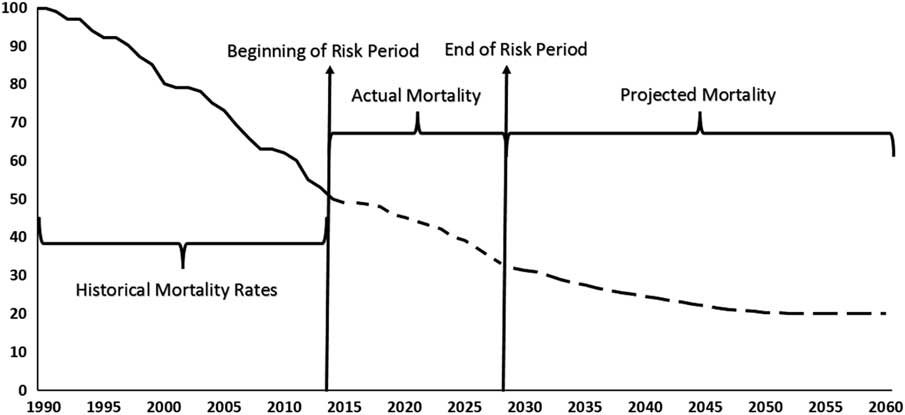
Figure 5 Mortality rates before, during and after the risk period
Note: Projected mortality rates are calculated using experience data available at end of the risk period.
Source: Michaelson & Mulholland (Reference Michaelson and Mulholland2014, Exhibit 3).
5.5.7. The hedge itself is structured using a long out-of-the money call option bull spread on future mortality outcomes. The spread has two strike prices or, using insurance terminology, an attachment point and an exhaustion point.Footnote 45 These strikes are defined relative to the distribution of “final index values” calculated using the agreed longevity model. The final index value will be a combination of:
∙ The “actual” mortality experience of the hedger throughout the risk period which is calculated by applying the reported national population mortality rates to the predefined “exposure vector” and “experience ratio matrix” for each cohort in each year of the risk period, and accumulating with interest, using forward interest rates defined on the trade date.
∙ The “commutation calculation” that estimates the expected net present value of the remaining exposure at the end of the risk period, calculated using the re-parameterised version of the initial longevity model.
5.5.8. Given the distribution of the final index, the attachment and exhaustion points are selected to maximise the hedger’s capital relief, taking into account the investors’ (i.e. risk takers’) wish to maximise the premium for the risk level assumed. Investors might also demand a “minimum premium” to engage in the transaction. The intermediary – e.g. the investment bank – therefore needs to carefully work out the optimal amount of risk transfer, given both the hedger’s strategic objectives and investor preferences.
5.5.9. The hedger then needs to calculate the level of capital required to cover possible longevity outcomes with a specified degree of confidence. For example, if the “best estimate” of the longevity liability is $1bn, the (re)insurer may actually be required to issue $1.2bn, $200 m of which is reserve capital to cover the potential increase in liability due to unanticipated longevity improvement with 99% confidence.
5.5.10. The (re)insurer may then decide to implement a hedge transaction with a maximum payout of $100 m. This transaction would begin making a payment to the hedger in the event the attachment point is breached, and then paying linearly up to $100 m if the longevity outcome meets or exceeds the exhaustion point. This hedge provides a form of “contingent capital” from investors (up to $100 m of the $200 m required), enabling the hedger to reduce the amount of regulatory capital it must issue – see Figure 6.
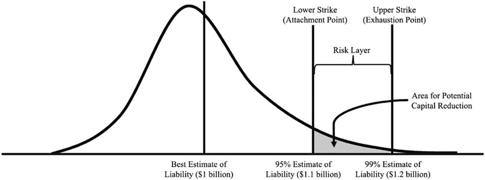
Figure 6 Distribution of the final index value and the potential for capital reduction
Source: Michaelson & Mulholland (Reference Michaelson and Mulholland2014, Exhibit 4) – not drawn to scale.
5.5.11. Tail risk protection was actually discussed in Living with Mortality in section 6.4 entitled “Geared Longevity Bonds and Longevity Spreads,” which we reproduce here. The geared longevity bond enables holders to increase hedging impact for any given capital outlay.
5.5.12. One way to construct such a bond would be as follows. Looking ahead from time 0, the payment on each date t can in theory range from 0 to 1 (times the initial coupon). However, again looking ahead from time 0, we can also suppose that the payment at time t (the survivor index, S(t,x); see paragraph 5.4.10 above) is likely to fall within a much narrower band, say S(t, x)∈[S l (t), S u (t)]. For example, if we are using a stochastic mortality model we could let S l (t) and S u (t) be the 2.5% and 97.5% percentiles of the simulated distribution of S(t, x). These simulated confidence limits become part of the contract specification at time 0.
5.5.13. We now set up a special purpose vehicle (SPV) at time 0 that holds S u (t)−S l (t) units of the fixed interest zero-coupon bond that matures at time t for each t=1,…,T (or its equivalent using floating-rate debt and an interest-rate swap). Suppose the SPV is financed by two investors A and B. At time t, the SPV pays: (i) S(t,x)−S l (t) to A with a minimum of 0 and a maximum of S u (t)−S l (t); and (ii) S u (t)−S(t,x) to B with a minimum of 0 and a maximum of S u (t)−S l (t).
5.5.14. The minimum and maximum payouts at each time to A and B ensure that the payments are always non-negative and can be financed entirely from the proceeds of the fixed-interest zero-coupon bond holdings of the SPV.
5.5.15. The payoff at t to A can equivalently be written as
 $$\left( {S\left( {t,x} \right){\minus}S_{l} (t)} \right){\plus}max\left\{ {S_{l} \left( t \right){\minus}S\left( {t,x} \right),0} \right\}{\minus}max\left\{ {S\left( {t,x} \right){\minus}S_{u} \left( t \right),0} \right\}$$
that is, a combination of a long forward contract, a long put option on S(t, x) (or a “floorlet,” with a strike price that is lower than the at-the-money forward rate), and a short call on S(t, x) (or a “caplet” with a strike price that is higher than the at-the-money forward rate). The bond as a whole, therefore, is a combination of forwards, floorlets and caplets. Continuing with the option terminology, we can also observe that the payoff to investor A is often referred to as a long “bull call spread,” and for this reason we refer to the payoff in the current context as a long “longevity bull call spread.”
5.5.16. Let us suppose that, for each t, S l (t) and S u (t) have been chosen so that the value of the floorlet and the caplet are equal. In this case, the price payable at time 0 by investor A is equal to the sum of the prices of the T forward contracts paying S(t, x)−S l (t) at times t=1,…,T. This is equal to (i) the price for the longevity bond paying S(t, x) at times t=1,…,T, minus (ii) the price for the fixed-interest bond paying S l (t) at times t=1,…,T. This structure therefore gives investors a similar exposure to the risks in S(t, x) for a lower initial price. For this reason, we describe the collection of longevity bull spreads as a geared longevity bond.
5.5.17. As an alternative, S u (t) might be set to 1, meaning that the caplet has zero value (S(t, x) cannot be bigger than 1). With this structure, investor A has full protection against unanticipated improvements in longevity, but gives away any benefits from poorer longevity than anticipated.
5.5.18. It is important to note in the above construction that there is a smooth progression in the division of the coupon payments between the counterparties over the range of S(t, x). This is preferable to a contract that has a jump in the amount of the payment as S(t, x) crosses some threshold: as often happens with such contracts as barrier options, arguments can often arise as to whether the particular threshold was crossed or not. Such difficulties are avoided with the smooth progression.
5.5.19. The bond described here is a variation on the Société Générale structure where the payoff at T depends only on the single survivor index S(T, x). In the more general case, the payoff depends on the values of S(1, x),…,S(T, x) and the forecast values at T of S(T + 1, x),S(T + 2, x),….
6. Index Versus Customised Hedges, and Basis Risk
6.1. Overview
Lucida and Canada Life implemented two very different kinds of capital markets longevity hedges in 2008. Lucida executed a standardised hedge linked to a population mortality index, whereas Canada Life executed a customised hedge linked to the actual mortality experience of a population of annuitants. Aegon’s hedges with Deutsche Bank in 2012 and with Société Générale in 2013 were also index hedges, but they were designed to minimise the basis risk involved.Footnote 46 It is important to understand the differences between index and customised hedges. It is also important to understand, measure and manage the basis risk in index hedges. This, in turn, will have implications for regulatory capital relief.
6.2. Index Versus Customised Hedges
6.2.1. Standardised index-based longevity hedges have some advantages over the customised hedges that are currently more familiar to pension funds and annuity providers. In particular, they have the advantages of simplicity, cost and greater potential for liquidity. But they also have obvious disadvantages, principally the fact that they are not perfect hedges and leave a residual basis risk (see Table 6) that requires the index hedge to be carefully calibrated.
Table 6 Standardised Index Hedges Versus Customised Hedges

Source: Coughlan (Reference Coughlan2007a).
6.2.2. Coughlan et al. (Reference Coughlan, Epstein, Sinha and Honig2007b) show that a liquid, hedge-effective market could be built around just eight standardised q-forward contracts with:
∙ a specific maturity (e.g. 10 years);
∙ two genders (male, female);
∙ four age buckets (50–59, 60–69, 70–79, 80–89).
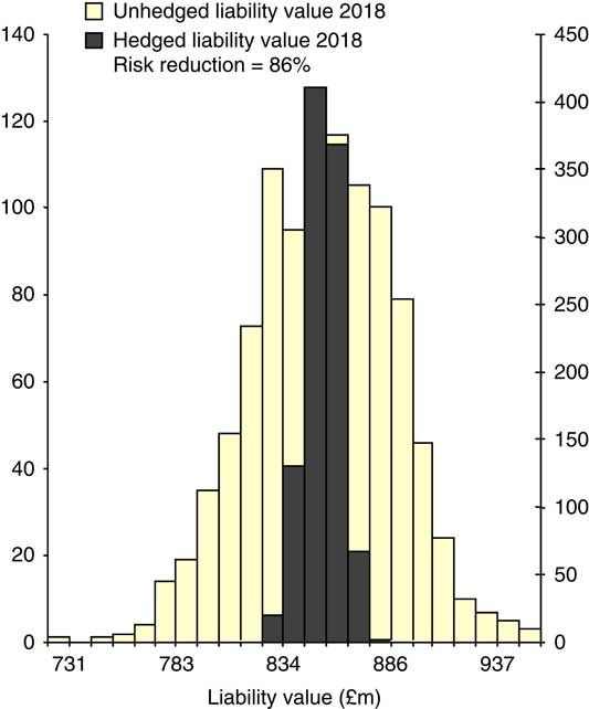
6.2.3. Figure 7 presents the mortality improvement correlations within the male 70–79 age bucket which is centred on age 75 (Coughlan et al., Reference Coughlan, Epstein, Ong, Sinha, Hevia-Portocarrero, Gingrich, Khalaf-Allah and Joseph2007c). These figures show that the correlations (based on graduated mortality rates) are very high. Consequently, a tailored hedge using, say, 10 q-forwards on ages 70–79 will be only marginally more effective than a single q-forward using a standard 70–79 age bucket. Coughlan (Reference Coughlan2007a) estimates that the hedge effectiveness (of a value hedge) is around 86% (i.e. the standard deviation of the liabilities is reduced by 86%, leaving a residual risk of 14%) for a large and well-diversified pension plan or annuity portfolio: see Figure 8.Footnote 47
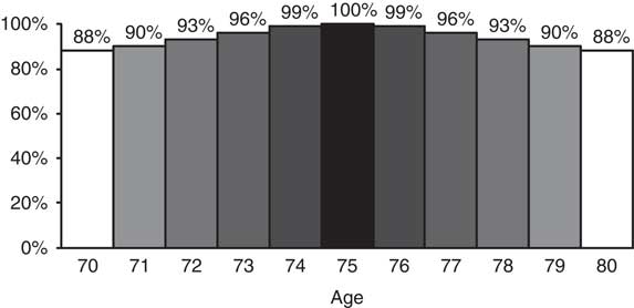
Figure 7 Five-year mortality improvement correlations with England & Wales males aged 75
Source: Coughlan et al. (Reference Coughlan, Epstein, Ong, Sinha, Hevia-Portocarrero, Gingrich, Khalaf-Allah and Joseph2007c, Figure 9.6).
6.2.4. In order to keep the number of contracts to a manageable level, individual contracts use the average (or “bucketed”) mortality across 10 ages rather than single ages. This averaging has positive and negative effects. On the one hand, the averaging reduces the basis risk that arises from the non-systematic mortality risk that is present in crude mortality rates, even at the population level.Footnote 48 On the other hand, it introduces some basis risk depending on the specific age-structure of the population being hedged. This we now discuss in more detail.
6.3. Basis Risk
6.3.1. Basis risk is the residual risk associated with imperfect hedging where the movements in the underlying exposure are not perfectly correlated with movements in the hedging instrument. Basis risk and its quantification have recently attracted the attention of both academics and practitioners (e.g. Li & Hardy, Reference Li and Hardy2011; Cairns et al., Reference Cairns, Blake, Dowd and Coughlan2014; Longevity Basis Risk Working Group, 2014; Villegas et al., Reference Villegas, Haberman, Kaishev and Millossovich2017; Li et al., Reference Li, Tickle, Tan and Li2017; Cairns & El Boukfaoui, Reference Cairns and El Boukfaoui2018).
6.3.2. Within the context of longevity risk hedging, a number of sources of basis risk arise: population basis risk; base-table risk; structural risk; restatement risk; and idiosyncratic risk.
6.3.3. Population basis risk is, perhaps, the form of basis risk that most readily comes to mind when considering an index based longevity hedge. Specifically, a hedger might choose to use a hedging instrument that is linked to a different population from its own population that it wishes to hedge. This is most common where the hedging instrument is linked to an index based on national mortality rates, while the hedger’s own population is a distinctive sub-population with different characteristics from the national average. As a consequence, underlying mortality rates might not just be at a different level from that of the national population, but rates of improvement in both the short and long term might not be perfectly correlated. Modelling and understanding the differences between two populations is an active and rapidly developing subject of research.Footnote 49
6.3.4. Base-table risk concerns how accurately hedgers and also receivers of longevity risk are able to assess the mortality base table for both the hedger’s own population and the national population. Whether or not base-table risk contributes to residual risk for the hedger then depends on the nature of the longevity hedge. At one end of the spectrum, from the perspective of the hedger, a customised longevity swap leaves the hedger with no base-table risk, while the receiver is exposed and should charge a higher price to reflect this extra risk. In contrast, for an index-based hedge, base-table risk will be relevant. Base-table risk will then make a more significant contribution to total basis risk if the hedger’s own population is small or the time horizon of the hedge is short.
6.3.5. Structural risk relates to the design of the hedging instrument, and it can arise even if there is no population basis risk or base-table risk:
∙ The hedging instrument might have a non-linear payoff as a function of the underlying risk. This includes contracts with an option-type payoff structure such as the bull call spread in Michaelson & Mulholland (Reference Michaelson and Mulholland2014) and Cairns & El Boukfaoui (Reference Cairns and El Boukfaoui2018), leaving residual risk both below and above the attachment and exhaustion points. It also includes q-forwards: these do not include any optionality, but liability cashflows are typically non-linear combinations of the underlying mortality rates.
∙ The hedging instrument might have a finite maturity, meaning that the longevity risk that emerges after the maturity date is a residual risk that cannot be hedged.
∙ The reference ages embedded in the hedging instruments might not allow exact matching of the ages in the hedger’s population.
∙ The number of units of the hedging instrument (i.e. the hedge ratio) might not be optimal (i.e. might not minimise residual risk). This might be either unavoidable or unintentional (e.g. through the use of a poorly calibrated model).
∙ Hedging instruments might not incorporate an inflation linkage and so might not match well with realised pension plan or annuity benefit increases.
In general, structural risk can be adjusted, for example, through the choice of: attachment and exhaustion points; the maturity date; the reference ages; the number of q- or S-forwards; and careful calibration and optimisation using the chosen stochastic mortality model.
6.3.6. Restatement risk concerns the possibility that official estimates of the national population or death counts might be revised up or down, with potential impacts on index-based hedge payoffs (Cairns et al., Reference Cairns, Blake, Dowd and Kessler2016). Restatements will often impact on previously stated mortality rates (especially following a decennial census). Index-based longevity hedges will probably link contractually to the first announcement of a mortality rate, meaning that the restatement of past mortality rates will not alter past payments and hence introduce an additional risk. However, restatements will also have an impact on future estimated population numbers and consequent mortality rates. The future risks and impacts of such restatements can be assessed through use of the same methodology for identifying phantoms proposed in Cairns et al. (Reference Cairns, Blake, Dowd and Kessler2016).
6.3.7. Idiosyncratic riskFootnote 50 is primarily linked to sampling variation and its financial impact within the hedger’s population. As with some other examples of basis risk, the impact of idiosyncratic risk will depend on the nature of the hedge (indemnity versus other forms). Given the evolution of the systematic risk in the underlying mortality rates, individuals will either die or survive independently of each other. Proportionately, this risk is larger for smaller pension funds. The level of idiosyncratic risk is also dependent on the heterogeneity in pension amounts (leading to concentration risk): for example, a 1,000-member pension plan in which 10% of the members are directors (or “big cheeses”) who generate 90% of the liabilities will be more risky than a 1,000-member plan with equal pensions.
6.3.8. Finally, as remarked in Cairns (Reference Cairns2014), accurate assessment of basis risk is one part of the process of choosing the best hedge. First, one needs to identify the different options for hedging.Footnote 51 Second, the risk appetite of the hedger needs to be properly assessed. Third, there needs to be an accurate assessment of the basis risk under each hedge. Fourth, prices need to be established for each hedge. Fifth, the combination of price, basis risk and risk appetite then point to a best choice out of all of the options available to the hedger.Footnote 52 Cairns (Reference Cairns2014) also highlights that no single hedging option is best for all pension plans. Everything else being equal, customised hedges are more likely to be preferred to index hedges by: smaller pension plans rather than larger (due to the greater idiosyncratic risk); and pension plan sponsors that are more risk averse. Also, certain hedging options (e.g. longevity swaps) are currently only available to pension plans with sufficiently large liabilities.
6.4. Other Types of Basis Risk
Other forms of basis risk might arise if a pension plan seeks to hedge the longevity risk associated with a group of active or deferred members, rather than retired members. These groups bring additional risks, including member options (such as lump sum commutation, trivial commutation, early/late retirement, increasing a partner’s benefits at the expense of the member’s benefits, and pension increase exchanges), partner status at retirement or member death and salary risk. The plan’s quantum of exposure to longevity risk depends on how these risks turn out, a risk that itself is not hedgeable.
7. Credit Risk, Regulatory Capital and Collateral
7.1. Overview
Another risk in Table 6 is counterparty credit risk. This is the risk that one of the counterparties to, say, a longevity swap contract defaults owing money to the other counterparty. When a swap is first initiated, both counterparties might expect a zero excess profit or loss.Footnote 53 But over time, as a result of realised mortality rates deviating from the rates that were forecast at the time the swap started, one counterparty’s position will be showing a profit and the other will be showing an equivalent loss. The insurance industry addresses this issue via regulatory capital and the capital markets deal with it via collateral.
7.2. Regulatory Capital
7.2.1. The regulatory regime covering insurance companies domiciled in the UK is governed by the Solvency II Directive which came into effect in January 2016 and is used to set regulatory capital requirements.
7.2.2. Regulatory capital is the level of capital or Own Funds required by an insurer’s regulatory authority, the PRA in the UK. Solvency II begins with a calculation of the insurer’s liabilities, known as technical provisions, which comprises a “best estimate” of the liabilities plus a risk margin – in the case where the liability cannot be reliably measured and/or suitably hedged. The sum of the best estimate and risk margin can be thought of as the market consistent value or fair value. On top of this, insurers must issue additional risk-based capital to meet first the Minimum Capital Requirement (MCR) and then the Solvency Capital Requirement (SCR).
7.2.3. A major objective of Solvency II is to value all assets and liabilities on a market-consistent basis and to ensure that the regulatory capital that insurance companies issue reflects all the unhedged risks on their balance sheets. The capital should be sufficient to ensure that an insurance company can either (i) survive the next 12 months with a 99.5% probability or (ii) survive a set of prescribed stress tests. The amount required can be determined using either a stochastic internal model or through the use of the standard stress test, which in the case of longevity risk is a sudden 20% reduction in mortality rates across all ages. For a 65-year old UK male, this corresponds approximately to a 1.5-year increase in life expectancy or a 7% increase in pension liabilities.
7.2.4. A consequence of any market-consistent approach is that both assets and liabilities are prone to market volatility. Insurance companies invest in long-term illiquid assets, like infrastructure, real estate and equity release mortgages, to reduce asset price volatility, and in corporate bonds to benefit from the credit and illiquidity premia embodied in their higher returns compared with government bonds.
7.2.5. In the case of long-term liabilities, such as annuities and buy-outs, short-term asset price volatility can be partially offset by “matching adjustments” (MAs). MAs are part of Solvency II regulations that depart from a market-consistent approach, by allowing insurersFootnote 54 to estimate the illiquidity premium – inherent in the asset portfolio if it contains such illiquid assets – to be added to the risk-free rate for the purposes of discounting liabilities. To do this, the insurer needs to allocate a specific pool of assets to the liability, where the assets are selected to match the cash-flow characteristics of the liability. The assets need to be matched for the entire term of the liability, in which case the liability can be valued using the higher but less volatile MA-adjusted discount rate. Because both the level and volatility of the liability calculated using this approach are now lower, lower levels of Own Funds and hence SCR are needed. However, because of longevity risk and the dearth of long-maturity longevity-linked assets available to hold in the portfolio, the asset match can never be perfect. The higher MA-adjusted discount rate is reduced somewhat to allow for this and the level of Own Funds correspondingly raised. A particular example is non-pensioner members of pension plans who have both greater longevity risk and more optionality than pensioner members. Both these factors lower the MA-adjusted discount rate and, by raising the level of Own Funds, increase the cost of providing deferred annuities to the pension plan or buying out this segment of the pension plan. Insurers also make use of reinsurance to reduce the volatility of liabilities and this will again have an effect on Own Funds.
7.2.6. One possible implication of Solvency II is that insurers might migrate away from the current cash-flow hedging paradigm towards the value-hedging paradigm. Specifically, insurers might aim to hedge their liability in one year’s time as a way to reduce their SCR under Solvency II. This requires comparison of liability and hedge instrument values one year ahead.
7.2.7. Despite Solvency II, some pension plans considering de-risking remain concerned about the financial strength of some insurers, which is why consultants, such as Barnett Waddingham, have launched an insurer financial strength review service, providing information on an insurer’s structure, solvency position, credit rating and key risks in their business model.
7.2.8. Regulatory capital deals principally with the credit risk of the insurer.Footnote 55 Conversely, the insurer faces credit risk from the pension plan in the case of, say, a longevity swap, and collateral would need to be posted to deal with this.
7.3. Collateral
7.3.1. The role of collateral is to reduce if not entirely eliminate counterparty credit risk in both capital market transactions and insurance contracts.
7.3.2. Collateral in the form of high-quality securities needs to be posted by the loss-making counterparty to cover such losses. However, the collateral needs to be funded and the funding costs will depend on the level of interest rates. Further, the quality of the collateral and the conditions under which a counterparty can substitute one form of collateral for another need to be agreed. This is done in the credit support annex (CSA) to the ISDAFootnote 56 Master Agreement that establishes the swap. The CSA also specifies how different types of collateral will be priced.
7.3.3. All these factors are important for determining the value of the swap at different stages in its life. Biffis et al. (Reference Biffis, Blake, Pitotti and Sun2016) use a theoretical model to show that the overall cost of collateralisation in mortality or longevity swaps is similar to or lower than those found in the interest-rate swaps market on account of the diversifying effects of interest rate and longevity risks – which are to a first order uncorrelated risks. In practice, agreeing the value of the collateral involves an iterative process. Valuing the fixed leg is generally straightforward, but there can be differences of opinion in valuing the floating leg. It is typical in reinsurance contract negotiations for both sides to recommend a basis. If the difference is too far apart, both sides agree to bring in either one or two external experts. If only one is used, both sides are bound by their assessment. If two are used and they are close, both sides agree to split the difference: if they are still too far apart, both sides will allow the experts to appoint an agreed third expert.
8. Liquidity
8.1. Liquidity is another important issue raised in Table 6. The key problem with customised solutions for some participantsFootnote 57 is that they are not liquid and cannot easily be reversed. By contrast, liquidity is a key advantage of deep and well-developed capital market solutions.
8.2. To ensure long-term viability, it is critical that a traded capital market instrument meets the needs of both hedgers and speculators (or traders). The former require hedge effectiveness, while the latter supply liquidity. However, liquidity requires standardised contracts. The fewer the number of standardised contracts traded, the greater the potential liquidity in each contract, but the lower the potential hedge effectiveness. There is therefore an important tradeoff to be made, such that the number of standardised contracts traded provides both adequate hedge effectiveness and adequate liquidity.
8.3. If they are ever to achieve adequate liquidity, it is likely that capital-markets-based solutions will have to adopt mortality indices based on the national population as the primary means of transferring longevity risk or sub-population indices that are transparent, trustworthy, reliable and durable. However, potential hedgers, such as life assurers and pension funds, face a longevity risk exposure that is specific to their own policyholders and plan members: for example, it might be concentrated in specific socio-economic groups or in specific individuals such as the sponsoring company’s directors. Hedging using population mortality indices means that life assurers and pension funds will face basis risk if their longevity exposure differs from that of the national population. Herein lies the tension between index-based hedges and customised hedges of longevity risk, and, in turn, the unavoidable trade-off between basis risk and liquidity.
8.4. The involvement of the capital markets would help to reduce the cost of managing longevity risk. This is because it should lead to an increase in capacity, together with greater pricing transparency (as a result of the activities of arbitrageursFootnote 58 ) and greater liquidity (as a result of the activities of speculators). These conditions should attract the interest of ILS investors, hedge funds, private equity investors, sovereign wealth funds, endowments, family offices and other investors seeking asset classes that have low correlation with existing financial assets. Longevity-linked assets naturally fit this bill.
8.5. Currently, there is still insufficient interest from these classes of investor. However, Figure 1 shows how the market might eventually come into balance, with increasing numbers of potential sellers of longevity risk protection attracted by a suitable risk premium to enter the market to meet the huge demands of potential buyers.
9. Mortality Models
9.1. Overview
It is clear from the solutions we have described above that mortality models play a critical role in their design and pricing (see, e.g. Figures 3 and 6). There are three classes of stochastic mortality model in use (with some models straddling more than one class):
∙ extrapolative or time series models;
∙ process-based models – which examine the biomedical processes that lead to death;
∙ explanatory or causal models – which use information on factors which are believed to influence mortality rates such as cohort (i.e. year of birth), socio-economic status, lifestyle, geographical location, housing, education, medical advances and infectious diseases.
Most of the models currently in use are in the first of these classes and we will concentrate on these in this section.
9.2. Extrapolative or Time Series Models – Single Population Variants
9.2.1. There are four classes of time-series-based mortality model in use. First is the Lee-Carter class of models (Lee & Carter, Reference Lee and Carter1992), which makes no assumption about the degree of smoothness in mortality rates across adjacent ages or years. Second is the Cairns–Blake–Dowd (CBD) class of models (Cairns, Blake & Dowd, Reference Cairns, Blake and Dowd2006), which builds in an assumption of smoothness in mortality rates across adjacent ages in the same year (but not between years).Footnote 59 Third is the P-splines model (Currie et al., Reference Currie, Durban and Eilers2004) which assumes smoothness across both years and ages.Footnote 60 Finally, there is the Age-Period-Cohort (APC) model which has its origins in medical statistics (Osmond, Reference Osmond1985; Jacobsen et al., Reference Jacobsen, Keiding and Lynge2002), and was first introduced in an actuarial context by Renshaw & Haberman (Reference Renshaw and Haberman2006). Other features have also jumped from one class to another with the resulting genealogy mapped out in Figure 9. The first two classes of models have also been extended to allow for a cohort effect.Footnote 61 All these models were subjected to a rigorous analysis in Cairns et al. (Reference Cairns, Blake, Dowd, Coughlan, Epstein, Ong and Balevich2009, 2011a) and Dowd et al. (Reference Dowd, Cairns, Blake, Coughlan, Epstein and Khalaf-Allah2010b, 2010c). The models were assessed for their goodness of fit to historical data and for both their ex-ante and ex-post forecasting properties.

Figure 9 A genealogy of stochastic mortality models
Source: Adapted from Cairns (Reference Cairns2014)
9.2.2. Cairns et al. (Reference Cairns, Blake, Dowd, Coughlan, Epstein, Ong and Balevich2009) used a set of quantitative and qualitative criteria to assess each model’s ability to explain historical patterns of mortality: quality of fit, as measured by the Bayes Information Criterion (BIC); ease of implementation; parsimony; transparency; incorporation of cohort effects; ability to produce a non-trivial correlation structure between ages; and robustness of parameter estimates relative to the period of data employed. The study concluded that a version of the CBD model allowing for a cohort effect was found to have the most robust and stable parameter estimates over time using mortality data from both England & Wales and the US. This model (usually referred to as “M7”) is now the keystone of one of the two approaches recommended by the Life and Longevity Markets Association (LLMA)Footnote 62 (Longevity Basis Risk Working Group, 2014, Villegas et al., Reference Villegas, Haberman, Kaishev and Millossovich2017, and Li et al., Reference Li, Tickle, Tan and Li2017).
9.2.3. Cairns et al. (Reference Cairns, Blake, Dowd, Coughlan, Epstein and Khalaf-Allah2011a) focused on the qualitative forecasting properties of the modelsFootnote 63 by evaluating the ex-ante plausibility of their probability density forecasts in terms of the following qualitative criteria: biological reasonableness;Footnote 64 the plausibility of predicted levels of uncertainty in forecasts at different ages; and the robustness of the forecasts relative to the sample period used to fit the models. The study found that while a good fit to historical data, as measured by the BIC, is a promising starting point, it does not guarantee sensible forecasts. For example, one version of the CBD model allowing for a cohort effect produced such implausible forecasts of US male mortality rates that it could be dismissed as a suitable forecasting model. This study also found that the Lee-Carter model produced forecasts at higher ages that were “too precise,” in the sense of having too little uncertainty relative to historical volatility. The problems with these particular models were not evident from simply estimating their parameters: they only became apparent when the models were used for forecasting. The other models (including the APC model) performed well, producing robust and biologically plausible forecasts.
9.2.4. It is also important to examine the ex post forecasting performance of the models. This involves conducting both backtesting and goodness-of-fit analyses. Dowd et al. (Reference Dowd, Cairns, Blake, Coughlan, Epstein and Khalaf-Allah2010b), undertook the first of these analyses. Backtesting is based on the idea that forecast distributions should be compared against subsequently realised mortality outcomes and if the realised outcomes are compatible with their forecasted distributions, then this would suggest that the models that generated them are good ones, and vice versa. The study examined four different classes of backtest: those based on the convergence of forecasts through time towards the mortality rate(s) in a given year; those based on the accuracy of forecasts over multiple horizons; those based on the accuracy of forecasts over rolling fixed-length horizons; and those based on formal hypothesis tests that involve comparisons of realised outcomes against forecasts of the relevant densities over specified horizons. The study found that the Lee-Carter model, the APC model and the CBD model (both with and without a cohort effect) performed well most of the time and there was relatively little to choose between them. However, another version of the Lee-Carter model allowing for a cohort effect repeatedly showed evidence of instability.Footnote 65
9.2.5. Dowd et al. (Reference Dowd, Cairns, Blake, Coughlan, Epstein and Khalaf-Allah2010c) set out a framework for evaluating the goodness of fit of stochastic mortality models and applied it to the same models considered by Dowd et al. (Reference Dowd, Cairns, Blake, Coughlan, Epstein and Khalaf-Allah2010b). The methodology used exploited the structure of each model to obtain various residual series that are predicted to be independently and identically distributed (iid) standard normal under the null hypothesis of model adequacy. Goodness of fit can then be assessed using conventional tests of the predictions of iid standard normality. For the data set considered (English & Welsh male mortality data over ages 64–89 and years 1961–2007), there are some notable differences amongst the various models, but none of the models performed well in all tests and no model clearly dominates the others. In particular, all the models failed to capture long-term changes in the trend in mortality rates. Further development work on these models is therefore needed. It might be the case that there is no single best model and that some models work well in some countries, while others work well in other countries.
9.2.6. The CBD model appears to work well in England & Wales for higher ages, and Figures 10–12 present three applications of the model using ONS data for England & Wales.

Figure 10 Longevity fan chart for 65-year-old English & Welsh males
Source: Own calculations.
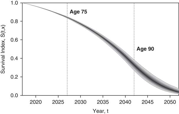
Figure 11 Cohort survivor fan chart for 65-year-old English & Welsh males
Source: Own calculations.

Figure 12 Cohort mortality fan chart for 65-year-old English & Welsh males
Source: Own calculations.
9.2.7. The first (Figure 10) is a longevity fan chart (Dowd et al, Reference Dowd, Blake and Cairns2010a), which shows the increasing funnel of uncertainty concerning future life expectancies out to 2052 of 65-year-old males from England & Wales.Footnote 66 By 2047, life expectancy from age 65 is centred around 23 years, shown by the dark central band: an increase of 4 years on the expectation for the year 2017. The different bands within the fan correspond to 5% bands of probability with the lower and upper boundaries at the 5% and 95% quantiles. Adding these together, the whole fan chart shows the 90% confidence interval for the forecast range of outcomes. We can be 90% confident that by 2047, the life expectancy of a 65-year-old English & Welsh male will lie between 21.3 and 24.3. This represents a huge range of uncertainty. Since every additional year of life expectancy at age 65 adds around 4–5%Footnote 67 to the present value of pension liabilities, the cost of providing pensions in 2060 could be 7–8% higher than the best estimate for 2047 made in 2017.
9.2.8. The second is a survivor fan chart (Blake et al., Reference Blake, Cairns and Dowd2008), which shows the 90% confidence interval for the survival rates of English & Welsh males who reached 65 at the end of 2016. Figure 11 shows that there is relatively little survivorship risk before age 75: a fairly reliable estimate is that 20% of this group will have died by age 75.Footnote 68 The uncertainty increases rapidly after 75 and reaches a maximum just after age 90, when anywhere between 27% and 38% of the original cohort will still be alive. We then have the long “tail” where the remainder of this cohort dies out some time between 2042 and 2062.
9.2.9. The third is a mortality fan chart which shows the 90% confidence interval for 65-year old English & Welsh males who reached 65 at the end of 2016. Figure 12 shows that there is an increasingly low probability of surviving year to year at very high ages, even with predicted mortality improvements.
9.2.10. By building off a good mortality forecasting model estimated using data from an objective, transparent and relevant set of mortality indices, fan charts provide a very useful tool for both quantifying and visually understanding longevity, survivor and mortality risks.
9.2.11. One key problem that extrapolative models have is their difficulty in differentiating between a genuine change in the trend of mortality rates and a temporary blip in mortality rates until some time after the change has occurred. In 2016, the UK Office for National Statistics reported that longevity improvements rates at very high ages have slowed down since 2011; but it is not yet clear whether this is a genuine change in the long-term trend, a short-term austerity-driven adjustment, or just the result of a purely random deviation from the previous trend.Footnote 69 Nevertheless, it prompted a debate in the UK in 2016 about the reliability of life expectancy projections. Mortality improvements in UK males averaged 0.6% p.a. over the preceding four years, compared with 3.2% p.a. in the decade before and 1.5–2% between 1995 and 2000.Footnote 70 In response to a possible trend change, the UK Continuous Mortality Investigation (CMI) has lowered its estimate of both male and female life expectancy at age 65 over 4 consecutive years, as Table 7 shows.
Table 7 UK Life Expectancy at Age 65

Source: Continuous Mortality Investigation.
9.2.12. In October 2016, Tim Gordon, head of longevity at Aon Hewitt, said: “This is the most extreme reversal in mortality improvement trends seen in the past 40 years. What was initially assumed by many actuaries to be a blip is increasingly looking more like an earlier-than-expected fall-off in mortality improvements. The industry is currently trying to digest all the implications of this emerging information and – inevitably – it is taking time to feed through into insurance and reinsurance pricing.” Others say that this could just be “noise.” Matt Wilmington, director of pension risk transfer at Legal & General (L&G), points out that: “Two years doesn’t make a trend – it’s very volatile from year to year. If we had another five years where we saw far fewer deaths than expected, then we might start to see fairly significant changes, but where we are now, there’s not enough to persuade us – or many of the pension plans we work with – that there’s a vast reversal in trend in terms of life expectancy just yet.” Despite this, Aon Hewitt said that there was sufficient dislocation in the pricing of longevity swaps that pension plans should consider delaying transactions until the market corrects. By the middle of 2017, Aon Hewitt reported that the longevity market was back in sync.Footnote 71 However, Tim Gordon also warned against attempts to time the market: “Timing the longevity market in the same way you would time an equity market is extremely difficult, and plans could be in danger of missing opportunities now if they did that.” The difference in mortality improvement rates before and after 2011 is equivalent to a difference in liabilities of 1% or 4 months of pension payments for every retiree: UK pension liabilities would be £25bn lower if the future mortality improvement rate were 1% rather than 3%.Footnote 72
9.2.13. Consultant Barnett Waddingham has put forward the suggestion that higher health and social care spending between 2000 and 2010 (which grew at an average annual real rate of 4%) may have caused a blip in longevity estimates by accelerating improvements. Since 2009, health spending has grown at just 1% per annum in real terms, social care spending has fallen in real terms, and there have been lower mortality improvements – although this correlation does not imply causation.Footnote 73
9.3. Extrapolative or Time Series Models – Multi-Population Variants
9.3.1. There are a number of reasons why it might be appropriate or desirable to model two or more populations simultaneously. First, a pension plan might often be relatively small in relation to the national population; it might have a relatively short run of data (e.g. relatively limited coverage of ages, or only a few calendar years of observations) or simply have a lot of sampling variation. In contrast, many national populations have a much longer run of data. By modelling the two populations in tandem and exploiting the correlations between the two, it might be possible to achieve better quality forecasts for the pension plan. Second, the use of multiple population mortality models enables more accurate modelling of the relationships between two or more groups that are directly of interest (e.g. males and females; assured lives and annuitants in a life insurer’s book of business; life insurance portfolios in different countries, etc.). This will lead to better consistency in forecasts as well as, for example, an assessment of the diversification benefits of having less-than-perfectly correlated groups of lives. Third, multi-population modelling is essential for any institution seeking to hedge its exposure to longevity risk using index-based hedging instruments: the model is required to assess the level of basis risk in the transaction.
9.3.2. The development of multi-population mortality models has lagged single population modelling quite considerably partly due to a lack of good quality sub-population datasets (the CMI assured lives dataset being a notable exception). The Human Mortality Database (HMD) has data for many countries and offers a useful starting point, but sub-population data present particular challenges that are often not present in international data (e.g. shorter runs of data, smaller population sizes, etc.). In the demography literature, Li and Lee (Reference Li and Lee2005) laid out some key foundations: in particular, the principle of coherence. The ratio of mortality rates in two populations can and will vary over time. However, the principle of coherence requires that this ratio should not diverge over time towards zero or infinity.Footnote 74 In the actuarial literature, key early contributions have been made by Cairns et al. (Reference Cairns, Blake, Dowd, Coughlan, Epstein and Khalaf-Allah2011b), Dowd et al. (Reference Dowd, Cairns, Blake, Coughlan and Khalaf-Allah2011), Li and Hardy (Reference Li and Hardy2011) and Börger et al. (Reference Börger, Fleischer and Kuksin2013).Footnote 75 More recently, Villegas et al. (Reference Villegas, Haberman, Kaishev and Millossovich2017) carried out an extensive review of both existing and potential new multi-population models. Despite the general popularity of the Li & Lee (Reference Li and Lee2005) model, their model has been found to be quite unsuitable for some actuarial applications by both Villegas et al. (Reference Villegas, Haberman, Kaishev and Millossovich2017) and Enchev et al. (Reference Enchev, Kleinow and Cairns2017). Specifically, applications that require a stochastic assessment of longevity risk (e.g. measurement of basis risk or diversification benefits) require models that have a plausible correlation term structure: the Li and Lee model fails on this criterion.Footnote 76
9.3.3. To satisfy the principle of coherence, Cairns et al. (Reference Cairns, Blake, Dowd, Coughlan, Epstein and Khalaf-Allah2011b) make use of a mean-reverting stochastic spread that allows for different trends in mortality improvement rates in the short-run, but parallel improvements in the long run. This study uses a Bayesian framework that allows the estimation of the unobservable state variables that determine mortality and of the parameters of the stochastic processes that drive those state variables to be combined into a single step. The key benefits of this include a dampening of the impact of Poisson variation in death counts,Footnote 77 full allowance for parameter uncertainty, and the flexibility to deal with missing data.
9.3.4. Dowd et al. (Reference Dowd, Cairns, Blake, Coughlan and Khalaf-Allah2011) employ a “gravity” model to achieve coherence using an iterative estimation procedure.Footnote 78 The larger population is modelled independently (similar to the approach recommended by Villegas et al., Reference Villegas, Haberman, Kaishev and Millossovich2017), but the smaller population is modelled in terms of spreads (or deviations) relative to the evolution of the larger population. To satisfy the principle of coherence, the spreads in the period and cohort effects between the larger and smaller populations depend on gravity or spread reversion parameters for the two effects. The larger the two gravity parameters, the more strongly the smaller population’s mortality rates move in line with those of the larger population in the long run.
9.3.5. In their comprehensive comparison of two-population models, Villegas et al. (Reference Villegas, Haberman, Kaishev and Millossovich2017) find that two models satisfy best their criteria for a good two-population model: the common age effect model (Kleinow, Reference Kleinow2015) with a cohort effect added; and a variant of the CBD family labelled as M7-M5.Footnote 79 Additionally, they offer useful guidance on the minimum quality of data for the sub-population: a minimum annual exposure of 20,000–25,000 lives over at least 8–10 years,Footnote 80 although Bayesian methods offer the potential to relax these criteria somewhat (e.g. Chen et al., Reference Chen, Cairns and Kleinow2017, Cairns et al., Reference Cairns, Blake, Dowd, Coughlan, Epstein and Khalaf-Allah2011b, Reference Cairns, Kallestrup-Lamb, Rosenskjold, Blake and Dowd2017a).
9.4. Process-Based and Causal Models
9.4.1. Until recently, these classes of models were not widely used, since the relationships between biomedical and causal factors and underlying death rates were not sufficiently well understood and because the underlying data needed to build the models were unreliable. This has begun to change.
9.4.2. In 2012, RMS launched a series of mortality indices and models via a platform called RMS LifeRisks. The platform allows life insurance companies and pension funds in the UK, the USA, France, Germany, Holland and Canada to model and manage their exposure to longevity and mortality risks, taking into account recent medical research and social change projections. There are two principal models.Footnote 81
9.4.3. The first model is the RMS longevity risk model. This is the base model used to project mortality and variations in mortality during normal conditions when there are no extreme mortality events. The projections depend on a number of so-called “vitagion categories” or individual sources of mortality improvement (see Figure 13). The five categories used by RMS are: lifestyle trends, including smoking prevalence; health environment; medical intervention; regenerative medicine, such as stem cell research, gene therapy and nanomedicine; and the retardation of ageing, including telomere shortening and caloric restriction.
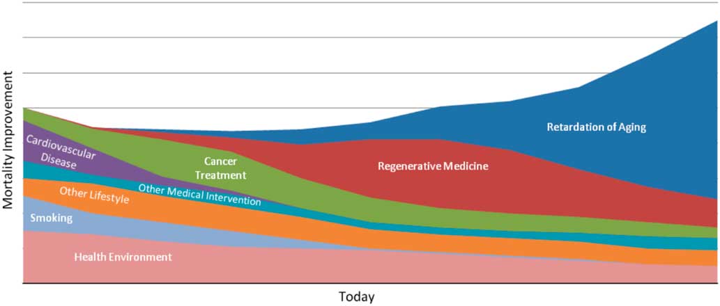
Figure 13 Timeline into the future
Note: Structural modelling of medical-based mortality improvement explores the timing, magnitude and impact of different phases of new medical advances on the horizon.
Source: RMS (2010) “Longevity Risk.”
9.4.4. The second model is the RMS infectious diseases model. This is used to estimate the additional mortality arising from the outbreak of certain infectious diseases, e.g. pandemic influenza. Both models were used in pricing the Kortis bond (see section 5.2) and an outbreak of something like influenza would be the most likely reason for the attachment point being reached during the life of the bond.
9.4.5. Academic researchers have recently begun experimenting with the introduction of causal variables in their mortality models (e.g. Hanewald, Reference Hanewald2011; Gaille & Sherris, Reference Gaille and Sherris2011; Alai et al., Reference Alai, Arnold (-Gaille) and Sherris2014a; Villegas & Haberman, Reference Villegas and Haberman2014; Gourieroux & Lu, Reference Gourieroux and Lu2015; Cairns et al., Reference Cairns, Kallestrup-Lamb, Rosenskjold, Blake and Dowd2017a). Practitioners also started to use post code as a measure of socio-economic class (SEC) in their proprietary mortality models, especially for pricing annuities. An early example is Richards (Reference Richards2008).
9.4.6. In 2008, Club Vita, a UK longevity data and analytics company, was set up with the express purpose of improving the socio-economic modelling of mortality data, allowing the segmentation of projections by SEC. To illustrate, cancer mortality related to smoking (such as larynx, oropharynx, oral cavity and lung) is more commonly associated with the lowest SEC, while cancer mortality related exposure to the sun (malignant melanoma) is more commonly associated with the highest SEC. Segmented longevity trend models have improved in recent years as a result of new insights from medical science and a greater understanding of cause of death for each SEC. The benefits of this to a pension plan have been an improved (and sometimes lower) best estimate of life expectancy (due to a more accurate socio-economic breakdown of the plan’s membership) with less uncertainty in the base table. The benefits to an insurer seeking new business have been refined pricing, better assessment of diversification, more effective risk selection, and increased competitiveness (Baxter & Wooley, Reference Baxter and Wooley2017). However, there is still an ongoing debate around using trend assumptions by SEC. For example, Jon Palin of Barnett Waddingham argues: “The evidence is less clear on the level of historical mortality improvements in pension schemes and other segments of the population, and to what extent a different assumption should be made for them.”Footnote 82
9.4.7. The emergence of new multi-population datasets with socio-economic subdivisions is also beginning to offer much greater potential for the development of reliable and robust multi-population models. For example, Cairns et al. (Reference Cairns, Kallestrup-Lamb, Rosenskjold, Blake and Dowd2017a) make use of Danish population data subdivided using a measure of affluence that combines wealth and income, and utilising this data, they develop a 10-population CBD-type stochastic model over the age range 55–94. With ten sub-populations to analyse, they avoid excessive model complexity by assuming a relatively simple model for correlations between sub-populations. A Bayesian framework is exploited to dampen the effect of sampling variation that is inherent in the ten relatively small sub-populations. It is anticipated that in the near future this and other datasets will become publicly available to allow researchers to develop alternative models, as well as further road-testing existing models.
10. Applications of the Mortality Models
10.1. Overview
In this section, we introduce some applications of the extrapolative mortality models introduced in the previous section: practical implementation of stochastic mortality models; determination of the longevity risk premium; estimating regulatory capital relief with a hedge in place; and comparison of alternative longevity risk management options. We begin by considering different types of users of these models.
10.2. Users of Stochastic Mortality Models
10.2.1. The following are potential users (directly or indirectly) of stochastic mortality models: insurers and reinsurers; regulators (e.g. the PRA); pension plans; specialist and general investors; actuaries and actuarial consultants; and software providers (e.g. Longevitas).
10.2.2. Insurers and reinsurers have a variety of reasons for using stochastic mortality models. Arguably, the principal reason is that they form part of an overall package of good enterprise risk management alongside stochastic models for other major risks, all augmented by a range of appropriate stress and scenario tests. Insurers can then use stochastic models to assess their economic capital requirements. Closely linked to this, many insurers are moving towards the use of stochastic models to assess regulatory capital requirements. For example, the PRA strongly encourages the use of stochastic mortality models with the standard one-year horizon under Solvency II (Prudential Regulatory Authority, 2015, 2016). Multi-population models also offer the potential for insurers to assess the diversification benefits resulting from exposure to different portfolios of lives (males/females, smokers/non-smokers, assurances/annuities, multi-country, etc.), with subsequent reductions, for example, in regulatory capital. Lastly, insurers might wish to use stochastic models to compare different options for the management of longevity risk. Depending on in-house capability, insurers might develop their own suite of stochastic mortality models, or use external expertise. This might come in the form of ready-to-use mortality software that is employed in-house by appropriately trained staff, or by contracting external consultants to perform stochastic analyses.
10.2.3. Regulators will not, typically, be direct users of stochastic mortality models. However, they do need to be sufficiently knowledgeable in their use (including awareness of the assumptions and limitations of each model) in order to be able to assess how they are being used by life insurers. Additionally, they need to be able to give periodic guidance on the use of stochastic models, including which models are, or are not, acceptable (see, for example Prudential Regulatory Authority, 2015, 2016).
10.2.4. The acceptance of systematic longevity risk will, in general, form part of the core risk taking activity of an insurer up to a level that is consistent with its overall risk appetite. In contrast, acceptance of longevity risk is not generally part of the core business of the typical sponsor of an occupational pension plan (nor indeed is investment and interest-rate risk). Nevertheless, systematic longevity risk is present and therefore requires careful attention. Large pension plans have the resources to assess their exposure to longevity risk through the use of both stochastic modelling and deterministic scenarios: again as part of a wider programme of integrated risk management. As with insurers, this might be done in-house, but more often this would be a service provided by the plan’s actuarial advisers. Smaller pension plans are less likely to have the financial resources to carry out a full stochastic assessment of longevity risk. However, there is the potential for the longevity risk research community to develop a small range of deterministic longevity scenarios (expressed as adjustments to the preferred best estimate forecast) that capture the essence of realistic extreme stochastic scenarios. On the other hand, consultancies now tend to have fairly streamlined processes for running off stochastic projections in order to illustrate the magnitude of each element of the longevity risk; these would typically be based on simplified pension benefits but would additionally reflect the most important aspects of the scheme, such as membership age, gender, and pension amounts. Such scenarios and projections should contrast favourably with the poorly formulated 20% stress test required under Solvency II (see Cairns & El Boukfaoui, Reference Cairns and El Boukfaoui2018). Models, therefore, can help plans determine appropriate target funding levels and contribution rates, as well as assess the risks associated with meeting these targets. Finally, as remarked earlier, use of stochastic models is recommended as a way to help choose between alternative longevity risk management options (including retention of the risk).
10.2.5. Pension plans also need to assess the potential future funding levels that might result from future uncertain investment returns, interest rate changes and changes in longevity. Stochastic mortality models can be used as part of a larger internal modelling exercise to assess uncertainty in funding levels. Larger plans will have the resources to carry out such an exercise. For smaller plans, stochastic models can again be used by actuarial consultants to generate a small number of deterministic extreme scenarios that can be applied to a range of smaller pension plans.
10.2.6. Specialist and general investors in longevity risk (e.g. ILS investors, hedge funds, private equity investors, sovereign wealth funds, endowments and family offices) and other receivers of longevity risk (e.g. reinsurers) are only likely to invest in this risk if it offers an acceptable risk premium, taking into account the low correlation between longevity risk and financial market risks and hence the potential diversification benefits from including longevity-linked products in an investment portfolio. This will be reflected in the price of the transaction at the outset relative to a best estimate or expected value. A rigorous approach to this requires a set of stochastic models to assess how much risk there is around the expected payoff.Footnote 83 In a competitive market, the size of the risk premium will reflect each potential investor’s other exposures: for example, a reinsurer might be satisfied with a lower risk premium for longevity risk if they have offsetting life assurance exposures.
10.3. Practical Implementation of Stochastic Mortality Models
10.3.1. It is common practice in the UK to use different methodologies for setting central forecasts and for risk assessment around that central forecast. For example, life insurers might use the CMI_2016 model (formally known as the CMI mortality projection model, calibrated using data up to 2016) to frame their central forecast and calculate best estimate liabilities. They then follow PRA guidelines (Prudential Regulatory Authority, 2015, 2016) and use stochastic mortality models to assess, proportionately, how much risk there is around that best estimate (Cairns et al., Reference Cairns, Blake and Dowd2017b). The use of CMI_2016 allows users some control over future improvement rates and, in key elements, requires the exercise of sound judgement (e.g. in setting the long-term rate of improvement). This contrasts with the more objective statistical approach prevalent in stochastic mortality modelling. Under the stochastic approach, the central forecast is determined by: the choice of model; the choice of time series model (or equivalent) for forecasting period and cohort effects; and the historical calibration period. These elements are ones that can be chosen objectively using standard statistical methods (see, for example Cairns et al., Reference Cairns, Blake, Dowd, Coughlan, Epstein, Ong and Balevich2009; Richards et al., Reference Richards, Currie, Kleinow and Ritchie2017). No further judgement is required once these selections have been made.
10.3.2. Current research is attempting to close the gap between the two approaches. For example, Richards et al. (Reference Richards, Currie, Kleinow and Ritchie2017) focus on the Age Period Cohort Improvements (APCI) model that underpins the historical calibration of the CMI_2016 model, and propose a coherent stochastic approach for forecasting. On the other hand, Cairns et al. (Reference Cairns, Blake and Dowd2017b) discuss an approach that closes the gap between the CMI central forecast and the mean trajectory under the objective statistical approach. This involves giving the user some control over setting the short and long term central trends in the period and cohort effects in a stochastic model. With some minor constraints applied to the historical calibration of the CMI model, the adapted stochastic model and the CMI_2016 projections can produce consistent central forecasts, allowing users to place greater reliance on the outputs of the stochastic model.
10.4. Determining the Longevity Risk Premium
10.4.1. As just discussed, the provider of any longevity hedge requires a premium to assume longevity risk. This means that the forward rate agreed at the start of any q-forward contract will be below the anticipated (expected) mortality rate on the maturity date of the contract. Similarly, the implied forward life expectancy in any longevity swap will be higher than the anticipated (expected) life expectancy. Figure 14 shows a typical relationship between the expected and forward mortality rate curves and the risk premium for a particular cohort currently aged 65.Footnote 84 Figure 15 shows the same for a particular age (in this case 65-year-old English & Welsh males) for years 2005–2025: the further into the future, the more uncertainty there is in the mortality rate and the bigger the risk premium.
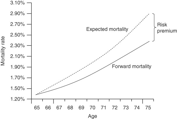
Figure 14 Cohort expected and forward mortality rate curves for a cohort currently aged 65 and q-forward maturity at age 75
Note: Lines are illustrative only.
Source: Adapted from Loeys et al. (Reference Loeys, Panigirtzoglou and Ribeiro2007, Chart 9).

Figure 15 Expected and forward mortality rate curves for 65-year-old English & Welsh males, 2005–2025
Note: Lines are illustrative only.
Source: Adapted from Coughlan (Reference Coughlan2007a).
10.4.2. As remarked above, a stochastic model can be used to assess how much uncertainty there is in the underlying hedge instrument, and then this information can be used to determine an appropriate risk premium. There are different approaches to setting the price, for example: discounting the expected payoff at an appropriate risk-adjusted discount rate that reflects the assessed level of risk; or calculating a risk-adjusted expected payoff prior to discounting at the risk-free rate. When applied to the pricing of multiple contracts, not all frameworks will produce consistent prices over a range of contracts and maturities. However, the method of risk adjustment proposed by Cairns et al. (Reference Cairns, Blake and Dowd2006) using an explicit market price of risk for each period effect and for each year is one that does guarantee pricing consistency. This can be used to determine what might be thought of as mid-market prices, around which participants in the market can set buying and selling prices that reflect the degree of market illiquidity.
10.5. Estimating Regulatory Capital Relief
10.5.1. In section 7.2 above, we discussed regulatory capital. Under Solvency II, an insurer’s regulatory capital can be reduced if its liabilities are appropriately hedged.
10.5.2. This necessitates bringing the relevant regulatory authority on board sooner rather than later, as experience in the Netherlands shows. The Dutch financial regulator, the Dutch National Bank (DNB), assesses longevity hedges on a case-by-case basis. A particular case is insurance, pensions and investments firm Delta Lloyd’s two index-based longevity hedges.Footnote 85 Delta Lloyd had its Solvency II capital ratio reduced by 14 percentage points at the end of 2015 following “intense discussions.” This was due to a disagreement with the DNB about the inclusion of risk margin relief on the two longevity hedges beyond the duration of the hedges. The DNB treats an index-based hedge as a financial instrument, whereas it treats a customised hedge as a reinsurance contract. It wanted the index-based hedges to be restructured to “ensure reinsurance treatment,” otherwise Delta Lloyd faced a further 7 percentage points deduction from its Solvency II ratio.
10.5.3. In June 2016, the DNB clarified its position. It agreed that for an index-based swap, capital relief will be proportional to the risk transfer. However, it felt that some previous index-based deals had been of too short duration, too out-of-the-money and not a good match for actual liabilities.Footnote 86
10.5.4. A detailed account of how to calculate regulatory capital relief in a longevity hedge can be found in Cairns and El Boukfaoui (Reference Cairns and El Boukfaoui2018).Footnote 87 They describe a flexible framework that blends practical issues with current academic modelling work. Key elements include careful assessment of basis risk, subdivided into population basis risk and other sources. They then consider a specific longevity hedge with a call option spread payoff structure and analyse the impact on regulatory capital. A key conclusion is that the balance between population basis risk and other sources of basis risk (especially structural basis risk) is highly dependent on the exhaustion point of the underlying option. For example, in a Solvency II setting, if the exhaustion point is close to the 99.5% quantile of the underlying risk, the recognition of population basis risk can have a significant effect on the regulatory capital required. In contrast, if the exhaustion point is somewhat below the 99.5% quantile (e.g. 95%), then population basis risk has a negligible impact on the amount of regulatory capital relief.Footnote 88 In the latter case, therefore, the index-based hedge acts in a very similar way to a reinsurance arrangement with similar attachment and exhaustion points in terms of its impact on regulatory capital. The authors conclude that hedgers need to consider carefully the terms of an index-based hedge (in the case considered, the attachment and exhaustion points and the maturity date), to ensure the best outcome. Further, in light of the evidence in the previous two paragraphs, insurers should discuss their plans with their local regulator before proceeding with a hedge. Bearing this in mind, Cairns & El Boukfaoui (Reference Cairns and El Boukfaoui2018) outline a clear set of steps that can be used to document regulatory capital relief calculations with the recommendation that these steps be followed as a way to facilitate discussions with local regulators. This includes a requirement to document clearly the structure of the two-population stochastic mortality model, how this is calibrated, how death rates get extrapolated to high ages, and how central forecasts will be determined at future valuation dates incorporating new information up to that valuation date.
10.6. Comparison of Risk Management Options
Good risk management practice includes consideration of a variety of viable options for reducing exposure to longevity risk, and stochastic models have a key quantitative role, alongside qualitative criteria, in the process that leads to choosing one option over another. Cairns (Reference Cairns2014) outlines some of the issues. The stochastic model can be used in a consistent way to evaluate a hedger’s longevity risk profile with and without each of the hedging options in place. The range of options itself might be constrained by the size of the liability to be hedged (for example customised longevity swaps have typically been restricted to larger pension plans) but should, in the first instance, include both customised and index-based hedges. Any analysis should also take into account a hedger’s exposure to idiosyncratic risk. Once residual risk has been evaluated, the hedger is then in a position to compare the different options. This should take into account the hedger’s general risk appetite as well as the underlying premium for a hedge (section 10.4) and future requirements for adjustments to the hedge (e.g. a buy-in used prior to a full buy-out). Cairns (Reference Cairns2014) discusses, in a stylised fashion, how these multiple inputs can result in different final decisions: one size does not fit all.Footnote 89
11. Developments in the Longevity Risk Transfer Market Since 2006
11.1. As mentioned at the beginning of this article, the global longevity de-risking market began in the UK in 2006. Prior to this time, the UK market was dominated by two life assurers, PrudentialFootnote 90 and L&G, which did business of approximately £2bn a year across a large number of small transactions. The total potential size of the UK market alone is around £2.7trn (on a buy-out basis) and this encouraged a raft of new players, in particular mono-line insurers, to enter the market.Footnote 91 The first of these was Paternoster, but others quickly followed including Pension Insurance Corporation (PIC), SynesisFootnote 92 and Lucida,Footnote 93 all of which were backed by investment banks and private equity investors. In 2007, Goldman Sachs established its own pension insurer, Rothesay Life. PaternosterFootnote 94 executed the first buy-out in November 2006 of the Cuthbert Heath Family Plan, a small UK plan with just 33 members. It also executed the first pensioner buy-in with Hunting PLC in January 2007.Footnote 95
11.2. The world’s first publicly announced longevity swap between Swiss Re and the UK life office Friends’ Provident in April 2007 (although this was structured as an insurance or indemnification contract rather than a capital market transaction). 2007 also saw the release of the LifeMetrics Indices covering England & Wales, the US, Holland and Germany by J. P. Morgan, the Pensions Institute and Willis Towers Watson (WTW) (then Towers Watson).Footnote 96 Xpect Age and Cohort Indices were launched in March 2008 by Deutsche Börse.Footnote 97 These indices cover, respectively, life expectancy at different ages and survival rates for given cohorts of lives in England & Wales, the USA, Holland and Germany and its regions. The purpose of these indices is to provide a benchmark for the trading of longevity-linked instruments. In 2009, longevity swaps began to be offered to the market based on Deutsche Börse’s Xpect Cohort Indices.
11.3. The world’s first capital market derivative transaction, a q-forward (or mortality forward) contract,Footnote 98 between J. P. Morgan and the UK pension fund buy-out company Lucida, took place in January 2008. The world’s first capital market longevity swap was executed in July 2008: Canada Life hedged £500 m of its UK-based annuity book (purchased from the defunct UK life insurer Equitable Life). This was a 40-year swap customised to the insurer’s longevity exposure to 125,000 annuitants. The longevity risk was fully transferred to investors, which included hedge funds and ILS funds. J. P. Morgan acted as the intermediary and assumes counter-party credit risk. In August 2011, ITV, the UK’s largest commercial TV producer, completed a £1.7bn bespoke longevity swap with Credit Suisse for its £2.2bn pension plan: the cost of the swap is reported as £50 m (3% of the notional swap value).Footnote 99 In February 2010, Mercer launched a pension buy-out index for the UK to track the cost charged by insurance companies to buy out corporate pension liabilities: at the time of launch, the cost was some 44% higher than the accounting value of the liabilities,Footnote 100 which highlights the attraction of using cheaper alternatives, such as longevity swaps, to transfer longevity.Footnote 101
11.4. On 1 February 2010, the Life and Longevity Markets Association (LLMA) was established in London. Its current members are Aviva, AXA, Deutsche Bank, J. P. Morgan, Morgan Stanley, Prudential, and Swiss Re. LLMA was formed to promote the development of a liquid market in longevity- and mortality-related risks.
11.5. This market is related to the ILS market and is also similar to other markets with trend risks, e.g. the market in inflation-linked securities and derivatives. LLMA aims to support the development of consistent standards, methodologies and benchmarks to help build a liquid trading market needed to support the future demand for longevity protection by insurers and pension funds. In April 2011, the LifeMetrics indices were transferred to LLMA with the aim of establishing a global benchmark for trading longevity and mortality risk.
11.6. In December 2010, building on its successful mortality catastrophe Vita bonds and taking into account the lessons learned from the failed EIB/BNP longevity bond, Swiss Re launched an 8-year longevity-spread bond valued at $50 m. To do this, it used a special purpose vehicle, Kortis Capital, based in the Cayman Islands. As with the mortality bonds, the longevity-spread bonds are designed to hedge Swiss Re’s own exposure to mortality and longevity risk. In particular, holders of the bonds face a reduction in principal if there is an increase in the spread between mortality improvements in 75–85-year-old English & Welsh males and 55–65-year-old US males, indicating that Swiss Re has life insurance (mortality risk) exposure in the USA and pension (longevity risk) exposure in the UK.Footnote 102
11.7. The world’s first longevity swap for non-pensioners (i.e. for active and deferred members of a pension plan) took place in January 2011, when J. P. Morgan executed a £70 m 10-year q-forward contract with the Pall (UK) pension fund. This was a value swap designed to hedge the longevity risk in the value of Pall’s pension liabilities, rather than the longevity risk in its pension payments as in the case of cash flow swaps – which have been the majority of the swaps that have so far taken place. Longevity risk prior to retirement is all valuation risk: there is no cash flow risk and most of the risk lies in the forecasts of mortality improvements at specific future valuation dates. Further, the longevity exposure of deferreds is not well defined as a result of the options that plan members have.
11.8. In 2011, WTW introduced the pension captive structure. A plan executes a pensioner buy-in with a standard insurer,Footnote 103 but then the insurer reinsures the buy-in with a captive insurer owned by the sponsor. Captives can provide a cost-effective solution compared with either a traditional buy-in or directly running the plan over the longer term. This is because there can be a more efficient blending of investment management services with insurance, combined with a more effective disaggregation of risks and hence a more capital-efficient management of those risks. The first plan to use this structure was Coca Cola in 2011 (Willis Towers Watson, 2017).
11.9. In December 2011, Long Acre Life entered the market to offer cheaper pension insurance solutions to larger plans with liabilities above £500 m. Under these solutions, companies offload their pension plans to an insurance vehicle in which they also invest and so share the profits along with external investors: the target return is 15% p.a.Footnote 104 In January 2012, L&G began offering longevity insurance (in the form of deferred buy-ins) for the 1,000 or so smaller plans with liabilities in the range £50-£250 m. In February 2012, UK pension consultant Punter Southall adopted PensionsFirst’s pension liability and risk management software (PFaroe) to automate the production of actuarial valuations and hence cut costs for pension plans, particularly small ones. In the same month, another UK consultant Hymans Robertson, launched a pension de-risking monitoring service which compares the costs of a full buy-out with the costs of a buy-in covering only pensioner members and the costs of a longevity swap.
11.10. The first pension risk transfers deals outside the UK took place in 2009–11. The first buy-in deal outside the UK was in 2009 in Canada; it was arranged by Sun Life Financial and valued at C$50 m. The first buy-in deal in Europe was in December 2010 between the Dutch food manufacturer Hero and the Dutch insurer Aegon (€44 m). The first buy-in deal in the USA (valued at $75 m) took place in May 2011 between Hickory Springs Manufacturing Company and the Prudential Insurance Co of America (PICA).Footnote 105 The first buy-out deal outside the UK was announced in May 2011 and involved the C$2.5bn Nortel pension plan in Canada. In September 2011, CAMRADATA Analytical Services launched a new pension risk transfer (PRT) database for US pension plans. The database provides insurance company organisational information, pension buy-in and buy-out product fact sheets and screening tools, pricing data, up-to-date information on each PRT provider’s financial strength and relevant industry research. Users can request pension buy-in and buy-out quotes directly from providers, including American General Life Companies, MetLife, Pacific Life, Principal Financial Group, PICA, Transamerica and United of Omaha.
11.11. The first international longevity reinsurance transaction took place in June 2011 between Rothesay Life (UK) and PICA (US) and was valued at £100 m. The first life book reinsurance swap since the Global Financial Crisis of 2007–2008 also took place in June 2011 between Atlanticlux and institutional investors and was valued at €60 m.
11.12. In February 2012, Deutsche Bank (through its insurance subsidiary Abbey Life) executed a huge €12bn index-based longevity swap for insurer Aegon in the Netherlands. This solution was based on Dutch national population data and enabled Aegon to hedge the liabilities associated with a portion of its annuity book (of €30bn). Deutsche Bank pays floating payments associated with the realised mortality rates of the reference index, but these payments are capped and floored. Aegon pays fixed premiums. The maturity of the swap is 20 years. A commutation mechanism determines the payment at maturity – the mechanism is designed to provide longevity protection for liability cashflows occurring beyond the 20-year maturity point. The swap has the structure of a series of call option spreads each with a long out-of-the money call at a strike price (or floor) and a short out-of-the money call at a higher strike price (or cap). Because the swap began deep out of the money (i.e. the floor is considerably higher than initial mortality rates), the amount of longevity risk actually transferred is far less than that suggested by the €12bn notional amount. Nonetheless, the key driver for this transaction from Aegon’s point of view was the reduction in regulatory capital it achieved. Most of the longevity risk has been passed to investors in the form of private bonds and swaps.Footnote 106
11.13. In June 2012, General Motors Co. (GM) announced a massive deal to transfer up to $26bn of pension obligations to PICA. This is by far the largest ever pension and longevity risk transfer deal globally. The transaction is effectively a partial pension buy-out involving the purchase of a group annuity contract for GM’s salaried retirees who retired before 1 December 2011 and refused a lump sum offer in 2012. To the extent retirees accepted a lump sum payment in lieu of future pension payments, the longevity risk was transferred directly to the retiree.Footnote 107 The deal was classified as a partial buy-out rather than a buy-in because it involved the settlement of the obligation. In other words, the portion of the liabilities associated with the annuity contract will no longer be GM’s obligation. Moreover, in contrast to a buy-in, the annuity contract will not be an asset of the pension plan, but instead an asset of the retirees. In October 2012, Verizon Communications executed a $7.5bn bulk annuity buy-in with PICA. The total buy-out deals market in the USA in 2012 amounted to $36bn.
11.14. The UK buy-outs for private sector pension plans had all involved plans that were closed to future accrual. However, in March 2012, PIC executed the first buy-out of a plan open to future accrual: the sponsoring employer, the high-tech manufacturer Denso, will pay PIC an annual premium based on the number of active members and their salaries, but PIC will assume all the liabilities. PIC had previously conducted an innovative buy-in in May 2011 with the London Stock Exchange’s DB pension plan which not only insured current pensioner members, but will also automatically insure active and deferred members when they reach retirement.
11.15. In June 2012, the OECD released the first edition of Pensions Outlook. This called on governments to kick-start the creation of a functioning longevity risk market and consider issuing longevity bonds, without which the annuity market is unlikely to work well. In September 2012, Swiss Re Europe released a report entitled A mature market: building a capital market for longevity risk. The report called for the development of a capital market for longevity risk. It said that “Society’s longevity risk could be tackled to a greater extent if reinsurers were able to expand their capacity, and this could be done by encouraging capital market investors to invest in longevity instruments. … The main challenges include achieving transparency in measuring the risk and potential liability, building a secondary market, increasing investor education, providing the right level of return and regulation.”Footnote 108
11.16. In December 2012, the enhanced buy-in market opened for business in the UK for DB pension plans. An enhanced buy-in is where a plan’s trustees buy a group annuity as an investment of the plan, where some or all of the members covered by the policy are medically underwritten. Medical underwriting, which is now commonplace in the individual annuity market (i.e. in relation to DC pensions), has the potential to reduce the cost to the plan of the longevity hedge compared with standard annuities, on the grounds that certain members might have lower than average life expectancy as a result of their lifestyle or some serious life-shortening illness. The market was introduced by two specialist insurers, Partnership and Just Retirement, but other larger insurers followed, e.g. L&G which offers a Large Individual Defined Benefit Annuity (LIBDA) service.
11.17. In February 2013, the first medically underwritten bulk annuity (MUBA) transaction was executed in the UK by Partnership (Harrison & Blake, Reference Harrison and Blake2013). This involved each member filling in a medical questionnaire in order to get a more accurate assessment of their life expectancy based on their medical history or lifestyle. This was particularly useful in the case of “top slicing,” where plan trustees insure the pensioners (who will typically be the company directors) with the largest liabilities and who therefore represent a disproportionate risk concentration for the plan. In December 2014, Partnership executed a £206 m medically underwritten bulk annuity transaction with a top slicing arrangement for the £2bn Taylor Wimpey pension plan. L&G transacted a £230 m medically underwritten buy-in in December 2015 with the Kingfisher Pension Scheme, covering 149 high-value members. The process of collecting medical information has been streamlined in recent years using third-party medical data collectors, such as MorganAsh, Age Partnership and Aon’s AHEAD platform – the first two of which also perform MUMS (medically underwritten mortality studies). New business more than doubled from £540 m in 2014 to £1,200 m in 2015, i.e. from 5% to 12.5% of the market (Hunt & Blake, Reference Hunt and Blake2016). In April 2016, the two largest UK medical underwriters, Partnership and Just Retirement – which both entered the market in 2012 – merged to form Just valued at £16bn. In December 2016, Just executed a £110 m medically underwritten buy-in with the Land Securities Group of Companies’ DB pension fund.
11.18. In April 2013, L&G reported its first non-UK deal, the buy-out of a €136 m annuity book from New Ireland Life. In June 2013, the Canadian Wheat Board executed a C$150 m pension buy-in from Sun Life of Canada, involving inflation-linked annuities, while in March 2014, an unnamed Canadian company purchased C$500 m of annuities from an insurer reported to be Industrial Alliance, making it the largest ever Canadian pension risk transfer deal to date.
11.19. In August 2013, Numerix, a risk management and derivatives valuation company, introduced a new asset class called “life” on its risk modelling platform (in addition to equities, bonds and commodities).
11.20. In September 2013, UK consultant Barnett Waddingham launched an insurer financial strength review service which provides information on an insurer’s structure, solvency position, credit rating, and key risks in their business model. This service was introduced in response to concerns about the financial strength of some buy-out insurers.
11.21. In November 2013, SPX Corp. of Charlotte, NC, purchased a buy-out contract with Massachusetts Mutual Life Insurance Co. as part of a deal that moved $800 m in pension obligations off SPX’s balance sheet.
11.22. Also in November 2013, Deutsche Bank introduced the Longevity Experience Option (LEO). It is structured as an out-of-the-money bull call option spread on 10-year forward survival rates and has a 10-year maturity. The survival rates are based on males and females in five-year age cohorts (between 50 to 79) derived from the England & Wales and Netherlands LLMA longevity indices. LEOs are traded over-the-counter under a standard ISDA contract. They allow longevity risk to be transferred between pension funds, insurance companies and investors. They are intended to provide a cheaper and more liquid alternative to bespoke longevity swaps which are generally costly and time consuming to implement. Purchasers of the option spread, such as a pension fund, will gain if realised survival rates are higher than the forward rates, but the gains will be limited, thereby providing some comfort to the investors providing the longevity hedge. The 10-year maturity is the maximum that Deutsche Bank believed investors will tolerate in the current stage in the development of a market in longevity risk transfers. It was reported that Deutsche Bank executed its first LEO transaction with an ILS fund in January 2014.Footnote 109
11.23. In December 2013, Aegon executed a second longevity risk transfer to capital markets investors and reinsurers, including SCOR. Société Générale was the intermediary in the deal covering liabilities of €1.4bn and RMS was the modelling agent. The main difference with the Deutsche Bank hedge is that there will be a single payment by Société Générale to Aegon if the swap is in-the-money at maturity (see section 5.5).
11.24. Also in December 2013, the Joint Forum reported on the results of its consultation on the longevity risk transfer market. It concluded that this market is not yet big enough to raise systemic concerns, but “their massive potential size and growing interest from investment banks to mobilise this risk make it important to ensure that these markets are safe, both on a prudential and systemic level” (Joint Forum, 2013, p.2).
11.25. In February 2014, the Mercer Global Pension Buy-out Index was introduced. It shows the benchmark prices of 18 independent third-party insurers in four countries with significant interest in buying out DB liabilities: UK, USA, Canada and Ireland. Costs were highest in the UK where the cost of insuring £100 m of pension liabilities was 123% of the accounting value of the liabilitiesFootnote 110 – equivalent to a price of £32 per £1 p.a. of pension (Towers Watson, 2015). The comparable costs in Ireland, the USA and Canada were 117%, 108.5% and 105%, respectively. The higher cost in the UK is in part due to the greater degree of inflation uprating of pensions in payment in the UK compared with the other countries. The difference between the USA and Canada is explained by the use of different mortality tables. Rising interest rates (following the unwinding of global quantitative easing programmes) and equity markets will lower funding deficits and hence lead to lower buy-out costs in future, especially in the USA.
11.26. In July 2014, Mercer and Zurich launched Streamlined Longevity Solution, a longevity swap hedge for smaller pension plans with liabilities above £50 m. This is part of a new Mercer SmartDB service which provides bespoke longevity de-risking solutions and involves a panel of reinsurers led by Zurich. It reduces the costs by having standardised processes for quantifying the longevity risk in each pension plan. The first deal, valued at £90 m, was transacted with an unnamed UK pension plan in December 2015. A second deal – this time with the UK pension plan of the Italian tyre company Pirelli – was executed in August 2016 for £600 m.
11.27. There is evidence of increasing demand from reinsurance companies for exposure to large books of pension annuity business to offset the risk in their books of life insurance.Footnote 111 For example, in July 2014, Warren Buffett’s Berkshire Hathaway agreed to a £780 m quota-reinsurance deal with PIC. Similarly, in August 2014, Delta Lloyd executed a 6-year index-based longevity swap covering €12 billion of its longevity reserves with RGA Re,Footnote 112 while AXA France executed a €750 m longevity swap with Hannover Re.
11.28. In March 2014, L&G announced the biggest single buy-out in the UK to date when it took on £3bn of assets and liabilities from ICI’s pension plan, a subsidiary of AkzoNobel. The deal uses “umbrella” contracts which enables the plan to add further liabilities onto the original contract.Footnote 113 In December 2014, L&G announced the largest ever UK buy-in valued at £2.5bn with US manufacturer TRW. In fact, in 2014, TRW became the first global corporation to simultaneously complete three de-risking transactions in three different countries: the UK, the USA and Canada. Also in 2014, the Aviva Staff Pension Scheme completed the first limited recourse longevity swap, involving £5 billion in liabilities and 19,000 participants.
11.29. Around £13bn of bulk annuity deals were executed in the UK in 2014, the largest volume of business since the de-risking market began in 2006 and beating the previous best year of 2008, just before the GFC, when £7.9bn of deals were completed. The total volume of de-risking deals in the UK in 2014 alone (covering buy-outs, buy-ins and longevity swaps) was £35bn. Included in this sum is the UK’s largest transaction to date, namely the longevity swap for the British Telecom (BT) Pension Scheme, covering £16bn of pension liabilities, arranged by PICA in July 2014. To complete the transaction, the BT scheme created its own captive insurer located in Guernsey, which insured the longevity risk. The captive insurer then reinsured the risk in a fully collateralised arrangement with PICA. This was the world’s first ever pension longevity captive transaction. Captive and limited recourse transactions have dominated the market since.
11.30. In December 2014, WTW launched Longevity Direct, an off-shore longevity swap hedging service that gives medium-sized pension plans with liabilities between £1–3bn direct access to the reinsurance market, via its own cell (or captive) insurance company. This allows plans to bypass (or pass through) insurers and investment banks – the traditional de-risking intermediaries – and significantly reduces transactions costs and completion times, while still getting the best possible reinsurance pricing. The first reported transaction on the Longevity Direct platform was the £1.5bn longevity swap executed by the Merchant Navy Officers Pension Fund (MNOPF) in January 2015 which was insured by MNOPF IC, a newly established cell insurance company based in Guernsey, and then reinsured with Pacific Life Re. In February 2015, PwC launched a similar off-shore longevity swap service for pension plans as small as £250 m. It uses a Guernsey-based incorporated cell company called Iccaria, established by Artex Risk Solutions, to pass longevity risk directly on to reinsurers. The arrangement is fully collateralised and each plan owns a cell within Iccaria which again avoids the costs of dealing with insurer and investment bank intermediaries. WTW also introduced the first tracking software system to follow live insurer pricing, sending alerts when a plan closes in on a target price.
11.31. In response to the announcement by the UK finance minister (George Osborne) in his Budget Speech on 19 April 2014, that UK pension plan members no longer needed to buy annuities when they retired (which resulted in an immediate fall in annuity sales of more than 50%), a number of traditional annuity providers, such as Scottish Widows, reported that they were considering entering the bulk annuity market.
11.32. In November 2014, the Longevity Basis Risk Working Group (2014) of the Institute & Faculty of Actuaries (IFoA) and LLMA published Longevity Basis Risk: A Methodology for Assessing Basis Risk.Footnote 114 This study develops a new framework for insurers and pension plans to assess longevity basis risk. This, in turn, will enable simpler, more standardised and easier to execute index-based longevity swaps to be implemented. Index-based longevity swaps allow insurers and pension plans to offset the systemic risk of increased liabilities resulting from members living longer than expected. It had hitherto been difficult to assess how effectively an index-based longevity swap could reduce the longevity risk in a particular insurance book or pension plan. The methodology they developed is applicable to both large plans (which are able to use their own mortality data in their models) and smaller plans (by capturing demographic differences such as socio-economic class and deprivation). In May 2016, a follow-up study – carried out by Macquarie University, Mercer Australia, and the University of Waterloo – was announced. The purpose was to design a “readily applicable methodology” for use with longevity risk indices: “Such indices are often used in pension benefits and annuitant liabilities, as well as in providing actuaries with key data, …but the problem of the existence of basis risk remains unsolved.” This follow-up study was published in December 2017 (Li et al., Reference Li, Tickle, Tan and Li2017). The report distinguishes between three types of basis risk (population, sampling and structural basis risk) and takes the proposed models in the 2014 report through to full analysis of hedge effectiveness. The report contains extensive numerical analyses that consider how hedge effectiveness depends on a range of input variables, including different book populations, size of book population, and type of hedge instrument, as well as the sensitivity to the underlying risk measure itself.
11.33. In March 2015, the UK government announced that it would introduce a new competitive corporate tax structure to allow ILSs to be domiciled in the UK. In May 2015, Rothesay Life, the insurance company owned by Goldman Sachs, bought out the liabilities of Lehman Brothers’ UK pension plan for £675 m, thereby securing the pensions of former employees of the company associated with the beginning of the GFC.
11.34. In April 2015, Swiss Re Capital Markets led the issuance of €285 m of excess mortality insurance-linked securities by Benu Capital Limited (Benu) on behalf of AXA Global Life. Swiss Re Capital Markets underwrote the transaction via two classes of principal-at-risk variable rate notes issued by Benu, an Irish private company incorporated with limited liability. The notes have a 5-year risk period starting on 1 January 2015. The proceeds of the notes each collateralise a counterparty contract with AXA Global Life, providing protection against excess mortality in France, Japan and the US via country age and gender weighted population mortality indices. It was the largest excess mortality issuance since 2007.Footnote 115
11.35. The largest buy-out to date in the UK was for the Philips Pension Fund which in November 2015 completed a full buy-out of the pension benefits of 26,000 members valued at £2.4bn with PIC. An interesting feature of this deal was that a buy-out was combined with a longevity hedge. The longevity risk was simultaneously reinsured with Hannover Re. Another interesting feature was that it covered both retired and deferred members, with the latter’s benefits valued at £1bn.
11.36. An important new longevity-linked product that recently took off in the UK was the equity release mortgage. This allows individuals to release equity in their homes to fund their retirement without downsizing. L&G, for example, set up L&G Home Finance for this purpose and in its first year completed more than £400 m equity release mortgage sales. Since equity release contracts typically involve a no negative equity guarantee,Footnote 116 the product provider is exposed to the risk that mortgagors live longer than expected.
11.37. In 2015, L&G directly entered both the USA and European pension risk transfer markets. It executed a $450 m transaction with the US subsidiary of Royal Philips covering 7,000 plan members in October and a €200 m deal with ASR Nederland NV, a Dutch insurer in December. The pension obligations were transferred to L&G Re in cooperation with Hannover Re. L&G said: “The pension risk transfer market has become a global business…The potential market for pension risk transfer in the US, UK and Europe is huge, and will play out over many decades.” Two US insurers were also involved in the Royal Philips deal: PICA acquired $450 m of plan liabilities covering another 7,000 members, while American United Life Insurance Company issued annuity contracts to 3,000 deferred plan members, valued at $200 m.
11.38. In January 2015, the Bell Canada Pension Plan executed a C$5bn longevity swap with Sun Life Financial,Footnote 117 SCOR, and RGA Re; it was SCOR’s first transaction in North America. In the process, Canada became the first country apart from the UK to have all three pension risk transfer solutions actively in use. In the same year, it completed its first inflation-linked buy-in annuity transaction, while in 2017 it completed its first buy-in annuity covering active future benefits.Footnote 118 In June 2015, Delta Lloyd did a second €12bn longevity swap with RGA Re: the swap was also index-based, with an 8-year duration and had a notional value of €350 m.Footnote 119 In July 2015, Aegon did one valued at €6bn with Canada Life Re, a new entrant to the de-risking market in 2015. Another new entrant was Scottish Widows.
11.39. In June 2015, the Mercer Pension Risk Exchange was launched. It gives clients in the USA, UK and Canada up to date buy-in and buy-out pricing based on their plan’s data. It collects prices provided monthly by insurers in the bulk market, based on plan benefit structures and member data. Mercer said: “Many companies have the appetite to transfer pension risk off their balance sheet, but they face barriers: lack of clear information about the true cost of a buy-in or buy-out, limited transparency, the fluctuation of market rates and plan economics to name but a few. [The exchange will enable] sponsoring employers and trustees to be more strategic and sophisticated in their approach and to know that they are executing a buy-in or a buy-out at the best time for them and at a competitive price.”
11.40. In April 2016, WTW released PulseModel which uses medical science and the opinions of medical experts to improve longevity predictions. For example, the model predicts that 16% of 50-year-old men in the UK will develop type-2 diabetes in the next 20 years, but this rises to 50% for those who are both obese and heavy smokers. Overall, the model predicts that longevity improvements in the future will be lower than currently predicted, at around 1% p.a. rather than 1.5%. If this turned out to be correct, then the current price of longevity of risk transfer products would be too high.
11.41. In 2016, there were a total of £8.6bn in buy-outs and buy-ins and £1.6bn in longevity swaps.Footnote 120
11.42. The largest buy-in in 2016 (in December) was Phoenix Life’s £1.2bn buy-in for the 4,400 pensioners in the PGL Pension Scheme, which is sponsored by the Phoenix Group, Phoenix Life’s parent company. This replaced a longevity swap it had set up for the plan in 2014. This is the first example of a transaction which transforms a longevity swap into a bulk annuity. Phoenix Life saw this as an opportunity to bring £1.2bn of liquid assets (mostly UK government bonds) onto its balance sheet, which could then be swapped into a higher yielding, matching portfolio, structured to maximise the capital benefit under Solvency II. This, in turn, meant that Phoenix Life would be assuming the market risks associated with the PGL scheme pension liabilities in addition to the longevity risks – and already does this on its existing book of individual annuities which are backed by £12bn of assets. The timing was also critical. Phoenix wanted to ensure that its internal model under Solvency II had bedded down well and that the capital and balance sheet impacts of the transaction were well understood, and that Phoenix had elicited the full support of the PRA for the transaction, thereby ensuring execution certainty. Phoenix also provided comfort to the plan’s trustees by giving them “all-risks” cover from point of buy-in (“all-risks” cover is not usually provided until buy-out) and strong collateral protection.Footnote 121
11.43. 2016 saw the beginning of a trend towards consolidation amongst insurance companies involved in the longevity risk transfer business in the UK. For example, Aegon sold its £9bn UK annuity portfolio to Rothesay LifeFootnote 122 and L&G between April and May, as part of a strategy to free up capital from non-core businesses. Part of the reason for this is the additional capital requirements under Solvency II.Footnote 123 Similarly, in September, Deutsche Bank sold its Abbey Life subsidiary to Phoenix Life – a consolidator of closed insurance books – for £935mn, as part of a planned programme of disposals aimed at restoring its capital base. There is an estimated £100bn of UK individual annuities in back books and further consolidation of these back books is anticipated. In December 2017, L&G sold its £33bn closed book of traditional insurance-based pensions, savings and investment policies to the ReAssure division of Swiss Re for £650 m.
11.44. Solvency II has also been blamed for some companies pulling out of the bulk annuities market altogether, a key example being Prudential in January 2016. Prudential is reported to be selling a portion of its £45bn UK annuity and pension liability businesses due to an inadequate return on capital and to transfer that capital to its growing businesses in Asia.Footnote 124 Reinsurance deals have also increased in response to Solvency II, involving non-EU reinsurers. For example, PIC executed a £1.6bn longevity reinsurance agreement with PICA in June 2016.
11.45. 2016 also witnessed the increasing streamlining and standardisation of contracts. This is particularly beneficial to small plans below £100 m. Previously, smaller plans have been less attractive to insurers due to the higher costs of arranging such deals relative to the profit earned. To circumvent this, consultants have begun offering services that allow smaller plans to access improved pricing and better commercial terms using a standardised off-the-shelf process incorporating pre-negotiated legal contracts. Pricing is more competitive because the insurer’s costs are kept low. An example is WTW’s Streamlined Bulk Annuity Service. The increasing maturity of the market has meant that some larger plans have also been prepared to use pre-negotiated contracts (Willis Towers Watson, 2017).
11.46. 2016 was also the tenth anniversary of the longevity transfer market. Since its beginning in the UK in 2006, £40bn of buy-outs and £31bn of buy-ins have taken place in the UK, covering 1 million people.Footnote 125 Yet this equates to just 5% of the £1.5trn of UK DB pension assets and 3% of the £2.7trn of DB pension liabilities on a buy-out basis. In addition, 48 longevity swaps are known to have been completed in the UK between 2007 and 2016, valued at £75bn and covering 13 insurance companies’ annuity and buy-out books, 22 private sector pension funds, and one local authority pension fund (some of which executed more than one swap).Footnote 126 Figure 16 shows the growth of the global market in longevity risk transfer between 2007 and 2017. A total of $366bn in transactions have been completed during this period.
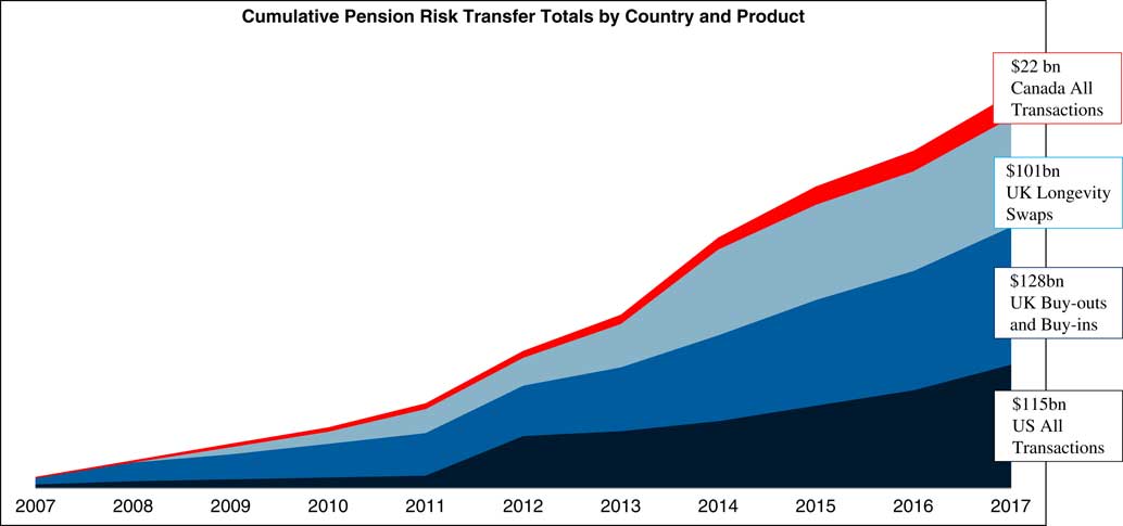
Figure 16 Cumulative pension risk transfers by product and country, 2007–17
Sources: LIMRA, Hymans Robertson, LCP and PFI analysis as of December 31, 2017.
11.47. At the beginning of 2017, there were eight UK-domiciled insurers actively participating in the pension risk transfer market in the UK. The largest players are PIC and Legal & General, with market shares of 37% and 30%, respectively. The others are Rothesay Life, Canada Life, Zurich, Scottish Widows, Standard Life, and new entrant Phoenix (since August). Occasionally, the insurers co-operate in a transaction. To illustrate, in August 2017, L&G executed a longevity swap in respect of £800 m of the pension liabilities of Scottish and Southern Energy (SSE), while PIC completed a £350 m buy-in for the company. Consultant LCP estimated that £12bn buy-ins and buy-outs took place in 2017 and predicts that £15bn will take place in 2018, with total insurer capacity at £25bn: “There remains significant capacity and competition – even if a large back-book comes to market – providing attractive opportunities for pension plans to transfer longevity risk through a buy-in or buy-out.”Footnote 127
11.48. One of the largest deals in 2017 (September) involved a £3.4bn longevity swap between the Marsh & McLennan Companies (MMC) UK Pension Fund and both Canada Life Reinsurance and PICA, using Guernsey-based incorporated cell companies, Fission Alpha IC Limited and Fission Beta IC Limited. MMC subsidiary Mercer led the transaction as adviser to the pension fund trustee and the deal was the first to be completed using the Mercer Marsh longevity captive solution, with no upfront premium. The two reinsurers shared the risk equally and the use of the captive ICC vehicle meant that no insurer intermediary was required, making the deal more cost-effective for the pension fund.Footnote 128 Also in September, the British Airways’ Pension Scheme used a similar Guernsey-based captive insurer to set up a £1.6bn longevity swap. The longevity risk was then reinsured with Partner Re and Canada Life Re. The scheme had previously hedged £2.6bn of liabilities through two longevity swap transactions executed by Rothesay Life in 2010 and 2011.Footnote 129 In November 2017, PIC executed a £900 m longevity swap with PICA, while in December 2017, L&G executed a £600 m longevity swap with PICA.Footnote 130
11.49. In December 2017, NN Life, part of the Nationale-Nederlanden Group, executed an index-based longevity hedge with reinsurer Hannover Re, in a deal covering the insurer against the longevity trend risk in €3bn of its liabilities. The structure is similar to the 2013 Aegon tail-risk deal arranged by Société Générale and builds on subsequent work including Michaelson & Mulholland (Reference Michaelson and Mulholland2014) and Cairns & El Boukfaoui (Reference Cairns and El Boukfaoui2018). While the term of the transaction is 20 years, NN Life is protected over a longer time period via a commutation functionFootnote 131 that applies at maturity. If longevity improvements have been much stronger than expected, this will be assumed to continue until the liabilities run-off and NN will receive a payment under the hedge. The transaction helped to reduce the solvency capital requirement of NN’s Netherlands life business by €35 m. The index attachment point for the hedge is close to NN’s best estimate, which helps maintain the SCR relief and effective risk transfer over time.Footnote 132 , Footnote 133
11.50. In April 2015, the UK government introduced “freedom and choice” pension reforms which gave more flexibility to how individuals could draw down their DC pension pots. In particular, there was no longer a requirement to purchase an annuity.Footnote 134 This immediately led to a fall in annuity sales by more than 50%. The situation was not helped by the fall in gilt yields (which led to a corresponding fall in annuity rates) arising from the government’s quantitative easing programme introduced after the GFC. In August 2017, a 65-year old with a £100,000 pension pot, could get a level income for life of £4,894: 2 years before, the amount would have been £5,292.Footnote 135 By 2017, the following insurers had pulled out of the open market for annuities: Aegon, LV=, Partnership (before it merged with Just Retirement to form Just), Prudential, Standard Life, Friends Life (merged with Aviva), Reliance Mutual, B&CE, and Retirement Advantage. This leaves just six providers left in what was once the world’s largest annuity market: Aviva (offering standard and enhanced annuities), Canada Life (standard and enhanced), Hodge Lifetime (standard only), Just (enhanced only), Legal & General (standard and enhanced) and Scottish Widows (standard only).Footnote 136
11.51. In order to reduce the costs of de-risking, pension plans are encouraged to perform some liability reduction exercises, the key ones being:Footnote 137
∙ Enhanced transfer values (ETVs) – allow deferred members to transfer an uplifted value of their benefits to an alternative arrangement. In August 2017, a 64-year old entitled to an index-linked pension starting at £10,000 from age 65 would be offered a transfer value of £237,000, according to the Xafinity Tranfer Value Index.Footnote 138
∙ Flexible retirement options (FROs) – allow deferred members aged 55 and over to retire early, or to take a transfer value and secure benefits in a different format from their plan benefits, or to use funds for drawdown purposes.
∙ Pension increase exchanges (PIEs) – allow pensioners to exchange non-statutory increases for a higher immediate pension with lower or even zero future increases (e.g. a £10,000 annual pension with RPI uplifting is replaced by a £12,000 annual pension with no further increases).
∙ Trivial commutations (TCs) – allow members with low value benefits to cash these in.
The most common exercises currently in the UK are PIEs and TCs – and these can be conducted either before or at the same time as a bulk purchase annuity broking exercise.
11.52. Innovation is a continuing feature of this market. Some examples include (see, e.g. Legal & General & Engaged Investor, 2016):
∙ Buy-ins and buy-outs with deferred premium payments – to spread costs.
∙ Phased de-risking using a sequence of partial buy-ins with an “umbrella” structure to avoid more than one set of contract negotiations – to spread costs.
∙ Accelerated buy-ins – the insurer provides a loan to the plan equal to the deficit (sometimes called a winding up lump sum (WULS)), so that a partial buy-in can take place immediately, with this converting to a full buy-in when the loan has been repaid, with the option of a full buy-out at a later date.
∙ Forward start buy-ins – a standard buy-in with the start date delayed to reflect the level of funding available, with additional options, such as paying deferred members as and when they retire if this is prior to the start date, or the ability to bring forward the start date for an additional fee.
∙ Automated bulk plan transfers – to reduce risks (introduced in November 2017 by Scottish Widows and Standard Life).Footnote 139
∙ Top-slice buy-ins – to target the highest value liabilities.
∙ Named-life longevity swap – if the named member lives longer than expected, the insurer pays out the difference (examples being the £400 m Bentley plan or an unnamed plan with 90 named pensioners valued at £50 m).
∙ Tranching by age – to reduce costs; according to consultant Punter Southall, a buy-in for pensioners up to age 70 will make a subsequent buy-out within the following 10 years cheaper than a buy-in for the over 70 s.Footnote 140
∙ Longevity swaps for small pension plans with liabilities of £50–100 m – previously only available for medium (£100–500 m) and large plans (above £500 m).
∙ Novation – the ability to transfer a longevity hedge from one provider to another, thereby introducing some liquidity into what had previously been a completely illiquid market. An example would be the reinsurance of a small bulk annuity transaction. Contract simplicity is a desirable feature of such arrangements.
∙ Longevity swap to buy-in conversions – as pioneered by Phoenix Life in December 2016 for its parent company’s pension plan. Solvency II incentivises buy-in providers to hold longevity insurance, otherwise they pay an additional risk margin. This encourages buy-in providers to seek out plans which already have a longevity hedge and encourage them to do a buy-in. Another driver is longevity swap providers that are not currently active in the market – such as J. P. Morgan and Credit Suisse – but are still responsible for running off their existing swaps. They might have an incentive to encourage the associated pension plan to novate the swap to a buy-in provider and hence extinguish their liability.Footnote 141
∙ Insuring away the extreme tail of liabilities in a closed plan after a specified term, such as 5 or 10 years – to reduce costs.
∙ Increasing optionality in contracts to improve flexibility – for example, the option to switch the indexation measure for pensions in payment from the Retail Price Index to the Consumer Price Index if government legislation changes; or the option to secure discretionary benefits, such as actual inflation above a 5% cap; or surrender options.
∙ Combining liability management solutions (such as interest rate and inflation swaps, and ETV, FRO and PIE exercises) and bulk annuities in a buy-out – so instead of completing liability management before considering a buy-out, plans do this in a single exercise.
∙ “Buy-out aware” investment portfolios – used to reduce buy-out price volatility and close the funding shortfall, with the buy-out price locked to the value of the buy-out aware funds once a target shortfall has been reached and whilst the contract documentation for a buy-out is being completed.
∙ Improved arrangements for handling data errors that arise after a deal has been executed – to reduce pre-deal negotiation requirements and post-deal transaction uncertainty. Common data errors include member gender, date of birth and benefit amounts for both member and partner. A simplified data error process could deal with these issues in the following way: locking down benefits, removing the need for re-pricing; mechanistically adjusting demographic errors; and using due diligence to check for systematic errors with the data.Footnote 142
∙ Arrangements to handle deferred members – to improve insurer appetite to assume the additional risk and cost involved. Deferred lives make up almost half (45%) of the membership of UK DB plans in the UK.Footnote 143 They are much more expensive to hedge for a number of reasons. First, there can be problems with their existence and identification. Second, they enjoy a large number of options which need to be priced.Footnote 144 Third, their longevity risk is greater, because the longevity improvement assumption used for pricing has greater reliance on the assumed long-run trend.Footnote 145 Fourth, as a direct consequence of the previous points, more capital is needed and this, in turn, increases the demand for reinsurance. These issues can be at least partially mitigated as follows: a robust existence checking procedure is needed involving electronic tracing, assuming a fixed percentage of the pension is exchanged for tax-free cash, setting the assumed retirement date to the plan’s normal retirement date, assuming no pension is exchanged for additional partner pension, restricting the age profile to older deferred members, and restricting the proportion of deferred members in the transaction.Footnote 146
11.53. These are all innovations in the space linking pension plans and insurance companies designed to ease the transfer of pension liabilities (or at least the longevity risk in them) from pension plans to insurance companies. But there is now an increasing sign of long-term capacity constraints within insurance companies.Footnote 147 As one consultant said: “Given the market has historically completed only 150–200 deals in any one year, there is a real risk of capacity constraints in the market, not just from an insurer capital perspective, but also from a resource and expertise perspective.”Footnote 148
11.54. In April 2017, the International Monetary Fund (IMF) released a new edition of its Global Financial Stability Report. Chapter 2 (“Low Growth, Low Interest Rates, And Financial Intermediation”) suggests that DB pension funds across the globe might have to cut benefits “significantly” in the long term because of ultra-low interest rates. Attempts to increase returns by changing asset allocations “appears feasible only by taking potentially unacceptable levels of risk.” In the face of such low rates, the IMF argues that “life insurers and pension funds would face a long-lasting transitional challenge to profitability and solvency, which is likely to require additional capital” or would require a “very high” level of volatility risk to meet their funding goals. However, a combination of risk aversion and regulatory constraints was likely to deter the vast majority from taking this second path. The IMF instead believes that the current situation might work to the benefit of insurers backing buy-ins and buy-outs. With investors increasingly monitoring the size of DB liabilities and the effects on company share prices, profits and dividends, the IMF said offloading these liabilities to insurers “is an attractive option” and “may represent a market-efficient arrangement” and that “regulation could play an important role in this area by facilitating such transactions.”
12. A Look into the Future: Potential Longevity Risk Transfer Solutions
12.1. Overview
A number of potential solutions were suggested in the 2006 Living with Mortality paper:
∙ Longevity bond types (e.g. zero-coupon longevity bonds, deferred longevity bonds, principal-at-risk longevity bonds and longevity spread bonds).
∙ Mortality, longevity and annuity futures.
∙ Mortality options, longevity caplets and floorlets.
∙ Mortality swaptions.
These were direct translations from already existing capital market instruments, but so far none of these, apart from a single longevity spread bond (i.e. Kortis) and a few longevity bull call spreads constructed using longevity caplets and floorlets (e.g. the 2013 Aegon deal with Société Générale), have been introduced in the longevity risk transfer market. In this section, we look at two potential new solutions that might have a greater chance of being introduced in the near term.
12.2. Potential New Solution: Longevity-Linked Securities
12.2.1. A perceived problem with the EIB/BNP Paribas longevity bond was that the reference index might not be sufficiently highly correlated with a hedger’s own mortality experience (as a result of population basis risk). An alternative instrument – denoted a longevity-linked security (LLS)Footnote 149 – deals, at least partly, with this problem. The concept was inspired by the design of mortgage-backed securities.
12.2.2. The LLS is built around a special purpose vehicle. Individual hedgers on one side of the contract (e.g. a pension plan or an annuity provider) arrange longevity swaps with the SPV using their own mortality experience at rates that are negotiated with the SPV manager. The swapped cashflows are then aggregated and passed on to the market. Bondholders gain if mortality is heavier than anticipated.
12.2.3. It might be felt that the aggregate cashflows themselves lack transparencyFootnote 150 in which case the SPV might link cashflows to an accepted reference index. The difference between this and the aggregated swap cashflows is a basis risk that is borne by the SPV manager.
12.2.4. This type of arrangement is illustrated in Figure 17 where the intermediary in this case is a reinsurer, which transacts customised longevity swaps with a set of hedgers. In this example, there are three hedgers, A, B and C (but there could, of course, be many more). Hedger A wishes to swap the risky longevity-linked cashflows L
A
(t) for a series of pre-determined cashflows. The agreement with the SPV manager is to swap floating L
A
(t) for fixed $\tilde{L}_{A} (t)$
for t=1,…,T, with the fixed leg set at a level that results in the swap initially having zero value at time 0. Similarly, hedger B swaps floating L
B
(t) for fixed
$\tilde{L}_{A} (t)$
for t=1,…,T, with the fixed leg set at a level that results in the swap initially having zero value at time 0. Similarly, hedger B swaps floating L
B
(t) for fixed $\tilde{L}_{B} (t)$
, and hedger C floating L
C
(t) for fixed
$\tilde{L}_{B} (t)$
, and hedger C floating L
C
(t) for fixed $\tilde{L}_{C} (t)$
. The SPV itself invests in AAA-rated, fixed-interest securities of appropriate duration or uses floating rate notes plus an interest-rate swap.
$\tilde{L}_{C} (t)$
. The SPV itself invests in AAA-rated, fixed-interest securities of appropriate duration or uses floating rate notes plus an interest-rate swap.
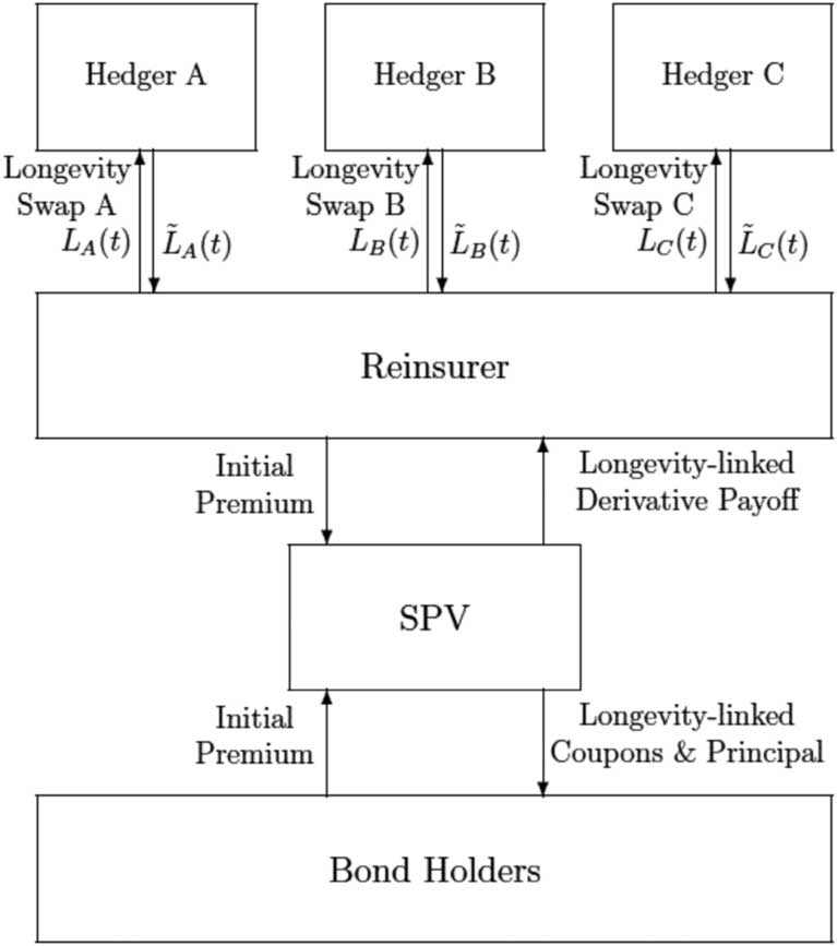
Figure 17 Cash flows under a LLS
12.2.5. The LLS bond holders pay an initial premium that is used to buy the fixed-interest securities and to pay an initial commission to the SPV manager. The bond holders in return receive coupons and, possibly, a final repayment of principal that is linked to a reference index, X(t), that matchesFootnote 151 as closely as possible the combined cashflows, rather than to L A (t), L B (t) or L C (t). Any differences accrue to or are paid by the SPV manager. The bond holders will not normally be hedgers themselves, so they will expect a fair premium over market fixed-interest rates in return for assuming the longevity risk.
12.2.6. Finally, the LLS might take the form of a catastrophe (or cat) bond (similar to the Kortis bond). In this case, the repayment of principal would be determined by the value of an index-based underlying, with appropriate attachment and exhaustion points.
12.2.7. To be more concrete, the underlying index X(t) that the LLS makes reference to is derived from, e.g. national population mortality rates, and is constructed in a way to achieve the optimal balance between hedge effectiveness for the reinsurer, within the cat bond structure, and the risk-return profile to investors. For a cat bond with attachment and exhaustion points AP and EP, the payoff at maturity will be the full bond nominal, N, if X(T) < AP, N(1−(X(T)−AP)/(EP−AP)) if AP≤X(T) < EP, and 0 if EP≤X(T).
12.2.8. The hedge is most likely to be effective if the reinsurer takes on a balanced and well diversified group of transactions with the primary hedgers (A, B and C above). For example, if the primary reinsurance transactions are wholly with blue collar pension plans, then an index-based LLS will be much less effective for the reinsurer. A low level of population basis risk turns out not to require exact matching of the national population (e.g. the aggregation of A, B and C). For example, Cairns et al. (Reference Cairns, Kallestrup-Lamb, Rosenskjold, Blake and Dowd2017a) demonstrate that an aggregated portfolio that covers 80% of the population but is also heavily skewed in value terms towards wealthier and healthier people can have a correlation with the national population that is well above 95%.
12.2.9. The marketing of LLS to ILS investors has great potential, following the introduction of comprehensive UK regulations for ILS in 2017, particularly if it takes the cat bond structure familiar to such investors, according to consultants Hymans Robertson. This is because longevity risk is becoming better understood and its volatility and correlation with other asset classes is low. Hymans Robertson argues that “Bulk annuity insurers could use [ILS] to provide additional capital to finance large deals (particularly where reinsurance is expensive or difficult to obtain) or to optimise their capital positions by rebalancing the risks on their balance sheets.” With the ILS investor base broadening all the time and an increasing amount of capital flowing into the market from other sophisticated investor sources, there is a growing pool of capital for which longevity or bulk-annuity linked risks might be attractive.Footnote 152
12.3. Potential New Solution: Reinsurance Sidecars
12.3.1. Another potential solution is the reinsurance sidecar – which is a way to share risks with new investors when the latter are concerned about the ceding reinsurer having an informational advantage.
12.3.2. Formally, a reinsurance sidecar is a financial structure established to allow external investors to take on the risk and benefit from the return of specific books of insurance or reinsurance business. It is typically set up by existing (re)insurers that are looking to either partner with another source of capital or set up an entity to enable them to accept capital from third-party investors (Kessler et al., Reference Kessler, Bugler, Nicenko and Gillis2016).
12.3.3. It is established as a SPV, with a maturity of 2–3 years. It is capitalised by specialist insurance funds, usually by preference shares, though sometimes in the form of debt instruments. It reinsures a defined pre-agreed book of business or categories of risk. Liability is limited to assets of the SPV and the vehicle is unrated.
12.3.4. The benefit to insurers is that sidecars can provide protection against exposure to peak longevity risks,Footnote 153 help with capital management by providing additional capacity without the need for permanent capital, and can provide an additional source of income by leveraging underwriting expertise. The benefit to investors is that they enjoy targeted non-correlated returns relating to specific short-horizon risks and have an agreed procedure for exiting; investors can also take advantage of temporary price hikes, but without facing legacy issues that could affect an investment in a typical insurer.
12.3.5. Figure 18 shows a typical sidecar structure.
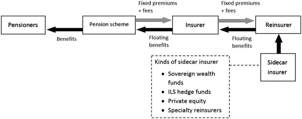
Figure 18 Typical sidecar structure
Source: PFI.
12.3.6. There are a number of challenges to the use of sidecars in the longevity risk transfer market. There is the tension between the long-term nature of longevity risk and investor preference for a short-term investment horizon. There are also regulatory requirements on cedants, affecting their ability to generate a return. These include: the posting of prudent collateral, the underlying assets in the SPV must generate matching cash flows, the risk transfer must be genuine, and the custodian/trustee must be financially strong. There is also a risk to cedants of losing capital relief if regulatory requirements are not met or they change.
12.4. Why Could These Potential Solutions Be Successful Now?
The principal reason why these solutions might be more successful now in a way that they were not a decade ago is the capacity constraint in the (re)insurance industry – it does not have the capital or experienced personnel to take on unlimited longevity risk. The only long-term solution to this capacity constraint is to bring in new investors from the capital markets (i.e. to transfer the risk to the capital markets). These investors will include ILS investors, hedge funds, private equity investors, sovereign wealth funds, endowments, family offices and other investors seeking asset classes that have low correlation with existing financial assets. However, two issues need to be resolved. First, the hedger needs assurance that the solution sold to these investors provides an effective hedge. Second, these investors need some assurance that they are not going to be sold a “lemon.”Footnote 154 There have been many attempts over the last decade to provide both types of assurance – without any real success. This time it might be – and certainly needs to be – different. An early sign of success for the reinsurance sidecar structure came at the beginning of 2018 when RGA Re and RenaissanceRe, announced a new start-up named Langhorne Re, which will target in-force life and annuity business. The new company has secured $780 m of equity capital from RGA, RenaissanceRe and third-party sidecar investors, including pension funds and other life companies.Footnote 155
13. Conclusions
13.1. As Michaelson & Mulholland (Reference Michaelson and Mulholland2014) point out:
the longevity risk inherent in the world’s aggregate retirement obligations is far in excess of the amount of risk capital the global insurance industry could realistically bring to bear against this risk.Footnote 156 Seen in this light, it becomes painfully obvious that vast sums of additional risk capital must be dedicated to adequately managing longevity risk. It is similarly evident that the only source capable of providing such quantities of capital, and thus assuming a meaningful amount of the world’s longevity risk, are the global capital markets…. The mission is clear – longevity risk must be successfully turned into an asset class capable of attracting these vast pools of capital, or else the world’s retirement systems will struggle to significantly reduce their longevity exposures in an efficient manner. However, developing capital markets solutions that are readily acceptable by a wide spectrum of institutional investors – given the complexity and uncertainty in modelling this long-term risk – requires innovative solutions from dedicated and experienced financial institutions.
There are four major challenges.
13.2. First, in order to expand the investor base, there is a need to close the gap between the preferences of stakeholders: buyers and sellers of longevity protection. Currently, long-term capital-market investors prefer bonds, while, as the paper has outlined, the most successful solutions have been longevity swaps. While short-term mortality bonds have been a success, long-term longevity bonds have not been similarly successful so far. So more creative approaches that develop a carefully structured risk management chain are needed to meet the differing requirements and risk appetites of stakeholders. However, the Swiss Re strategy of gradual iteration from a successful innovation – as exemplified in the Kortis longevity spread bond which was a modest adaptation of the Vita mortality bond in terms of design and maturity – appears to show a way forward, as do elements of the recent NN Life transaction in the Netherlands. The two key prizes, if successful, are a much bigger investor base and much greater market liquidity.
13.3. Second, there needs to be a common agreement between market participants on which mortality model to use for the design and pricing of each longevity-linked deal. One of the main reasons why Aegon’s deal with Société Générale went ahead in 2013 was that all parties agreed to use the same mortality model. Even if a mortality model produces the wrong forecasts – which it is bound to do – as long as those forecasts are not systematically biased, then it becomes a potential candidate for use in this market.
13.4. Third, a number of operational issues need to be dealt with. These include basis risk, credit risk, collateral and liquidity. Not only will this require market participants to work out the optimal trade-offs between basis risk and liquidity and between credit risk and collateral, it will also require the regulator to be willing to grant fair levels of regulatory capital relief for index-based hedge solutions that are compatible with current solvency capital requirements and consistent with levels of capital relief for customised longevity hedges, thereby putting both types of hedge on a level footing.
13.5. Fourth, it is important to engage with the regulator. This was the key message of Richard Sandor, a serial starter of new markets, such as the financial futures, climate exchange and Ameribor markets,Footnote 157 when he spoke at the Longevity 12 conference in September 2016.Footnote 158 He said that he always worked closely with the regulator when he was introducing a new product or market, so that there would be no surprises on the launch date. Failure to do this in the case of some of the early Dutch tail-risk protection deals meant that the Dutch regulator did not give the capital relief that was anticipated at the design stage. Regulators can also have big unintended consequences if, instead of engaging with them, there are attempts to circumvent them. For example, regulatory responses to the Global Financial Crisis (such as the US Dodd-Frank Act) had a significant effect in slowing down the establishment of longevity-linked capital market securities – which had nothing to do with the crisis itself. Regulations restricting the risk-taking activities of investment banks and new bank capital rules (Basel III) severely limited the role that banks could play in the development of this market. For example, it became virtually impossible for them to warehouse risk while matching longevity hedgers and longevity investors; and it even became unattractive for them to intermediate, standing in the middle between hedgers and investors, because the long-dated, illiquid credit exposure associated with longevity transactions now carried increased capital requirements.Footnote 159 While significant parts of the Dodd-Frank Act are in the process of being repealed, there is little sign that investment banks – the traditional conduit for introducing new capital from global investors, such as sovereign wealth funds – are returning to the longevity risk market.
13.6. These four challenges will need to be addressed in the next stage of the development of this market. But innovation has been an important feature of the longevity market since 2006 and there is every reason to believe that this will continue as the different players in the industry seek to meet the growing demand for longevity risk transfers, while reducing costs, optimising capital and managing risks.
Acknowledgements
The authors acknowledge funding from the Actuarial Research Centre of the Institute and Faculty of Actuaries through the “Modelling Measurement and Management of Longevity and Morbidity Risk” research programme, the Society of Actuaries and the Canadian Institute of Actuaries. The authors would also like to thank the two scrutineers of the paper for their extremely helpful and detailed comments on an earlier version of the paper.


 Open access