2.1. Intermediate model

We choose to model the key random quantities as integer-valued random variables with conditional distributions that are either Poisson or Negative Binomial distributions. Other choices of distributions on the integers are possible without any major effects on the analysis that follows. Let

(2.3) \begin{align}\mathcal{L}\!\left(N_{t+1}\mid \mathcal{F}_t\right)=\mathcal{L}(N_{t+1}\mid P_t)=\textsf{Pois}\!\left(aP_t^{b}\right),\end{align}

where $a>0$ is a constant, and $b<0$ is the price elasticity of demand. The notation says that the conditional distribution of the number of contracts written during year $t+1$ given the information at the end of year t depends on that information only through the premium decided at the end of year t for those contracts.

Let $\widetilde{N}_{t+1}=(N_{t+1}+N_t)/2$ denote the number of contracts during year $t+1$ that provide coverage for accidents during year $t+1$ . Let

(2.4) \begin{align}\text{OE}_{t+1}=\beta_0 +\beta_1 \widetilde{N}_{t+1},\end{align}

saying that the operating expenses have both a fixed part and a variable part proportional to the number of active contracts. The appearance of $\widetilde N_{t+1}$ instead of $N_{t+1}$ in the expressions above is due to the assumption that contracts are written uniformly in time over the year and that accidents occur uniformly in time over the year.

Let $\alpha_1,\dots,\alpha_4\in [0,1]$ with $\sum_{i=1}^4\alpha_i = 1$ . The constant $\alpha_k$ is, for a given accident year, the expected fraction of claim costs paid during development year k. Let

(2.5) \begin{align}\mathcal{L}\!\left(I_{t,k}\mid \mathcal{F}_{t},\widetilde{N}_{t+1}\right)=\mathcal{L}\!\left(I_{t,k}\mid \widetilde{N}_{t+1}\right)=\textsf{Pois}\!\left(\alpha_k\mu\widetilde N_{t+1}\right),\end{align}

where $\mu$ denotes the expected claim cost per contract. We assume that different incremental claims payments $I_{j,k}$ are conditionally independent given information about the corresponding numbers of contracts written. Formally, the elements in the set

\begin{align*}\left\{I_{j,k}\,:\,j\in\{t-l,\dots,t\}, k\in \{1,\dots,4\}\right\}\end{align*}

are conditionally independent given $N_{t-l},\dots,N_{t+1}$ . Therefore, using (2.1) and (2.5),

(2.6) \begin{align}\mathcal{L}\!\left(\text{PC}_{t+1}\mid \mathcal{F}_t, \widetilde{N}_{t+1}\right) &=\mathcal{L}\!\left(\text{PC}_{t+1}\mid \widetilde{N}_{t-2},\dots,\widetilde{N}_{t+1}\right)=\textsf{Pois}\!\left(\alpha_1\mu \widetilde{N}_{t+1}+\dots+\alpha_4\mu \widetilde{N}_{t-2}\right),\nonumber \\\text{IC}_{t+1}-\text{RP}_{t+1}&=\text{PC}_{t+1}+\left(\alpha_2+\alpha_3+\alpha_4\right)\mu \widetilde{N}_{t+1} - \alpha_2\mu \widetilde{N}_t-\alpha_3\mu \widetilde{N}_{t-1}-\alpha_4\mu \widetilde{N}_{t-2}. \end{align}

The model for the investment earnings $\text{IE}_{t+1}$ is chosen so that $G_t\leq 0$ implies $\text{IE}_{t+1}=0$ since $G_t\leq 0$ means that nothing is invested. Moreover, we assume that

(2.7) \begin{align}\mathcal{L}(\text{IE}_{t+1}+G_t\mid \mathcal{F}_t,G_t>0)=\mathcal{L}(\text{IE}_{t+1}+G_t\mid G_t,G_t>0)=\textsf{NegBin}\bigg(\nu G_t,\frac{1+\xi}{1+\xi+\nu}\bigg),\end{align}

where $\textsf{NegBin}(r,p)$ denotes the negative binomial distribution with probability mass function

\begin{align*}k\mapsto \binom{k+r-1}{k}(1-p)^{r}p^k\end{align*}

which corresponds to mean and variance

\begin{align*}\operatorname{E}\![\text{IE}_{t+1}+G_t\mid G_t,G_t>0] & = \frac{p}{1-p}r = (1+\xi)G_t,\\[4pt]\operatorname{Var}(\text{IE}_{t+1}+G_t\mid G_t,G_t>0) & = \frac{p}{(1-p)^2}r=\frac{1+\xi+\nu}{\nu}(1+\xi)G_t.\end{align*}

Given a premium rule $\pi$ that given the state $S_t=(G_t,P_{t-1},N_{t-3},N_{t-2},N_{t-1},N_t)$ generates the premium $P_t$ , the system $(S_t)$ evolves in a Markovian manner according to the transition probabilities that follows from (2.3)–(2.7) and (2.2). Notice that if we consider a less long-tailed insurance product so that $\alpha_3=\alpha_4=0$ (at most one year delay from occurrence of the accident to final payment), then the dimension of the state space reduces to four, that is $S_t=(G_t,P_{t-1},N_{t-1},N_t)$ .

2.2 Simple model

Consider the situation where the insurer has a fixed number N of policyholders, who at some initial time point bought insurance policies with automatic contract renewal for the price $P_t$ year $t+1$ . The state at time t is $S_t=(G_t,P_{t-1})$ . In this simplified setting, $\text{OE}_{t+1}=\beta_0+\beta_1 N$ , all payments $I_{t,k}$ are independent, $\mathcal{L}(I_{t,k})=\textsf{Pois}(\alpha_k\mu N)$ , $\text{IC}_{t+1}-\text{RP}_{t+1}=\text{PC}_{t+1}$ and $\mathcal{L}(\text{PC}_{t+1})=\textsf{Pois}(\mu N)$ .

2.3 Realistic model

In this model, we change the distributional assumptions for both investment earnings and the incremental claims payments from the previously used integer-valued distributions. Let $(Z_{t})$ be a sequence of iid standard normals and let

\begin{align*}\mathcal{L}\!\left(\text{IE}_{t+1}+G_t \mid G_t,G_t>0\right) = \mathcal{L}\!\left(G_t\exp\{\widetilde \mu + \widetilde\sigma Z_{t+1}\}\mid G_t,G_t>0\right).\end{align*}

Let $C_{t,j}$ denote the cumulative claims payments for accidents occurring during year $t+1$ up to and including development year j. Hence, $I_{t,1}=C_{t,1}$ , and $I_{t,j} = C_{t,j}-C_{t,j-1}$ for $j>1$ . We use the following model for the cumulative claims payments:

(2.8) \begin{align}C_{t,1}&=c_0\widetilde{N}_{t+1}\exp\!\left\{\nu_0Z_{t,1}-\nu_0^2/2\right\}, \nonumber\\[4pt]C_{t,j+1}&=C_{t,j}\exp\!\left\{\mu_j+\nu_jZ_{t,j+1}\right\}, \quad j=1\dots,J-1,\end{align}

where $c_0$ is interpreted as the average claims payment per policyholder during the first development year, and $Z_{t,j}$ are iid standard normals. Then,

\begin{align*}\operatorname{E}\!\left[C_{t,j+1}\mid C_{t,j}\right]&=C_{t,j}\exp\!\left\{\mu_j+\nu_j^2/2\right\}, \\[5pt]\operatorname{Var}\!\left(C_{t,j+1}\mid C_{t,j}\right)&=C_{t,j}^2\left(\exp\!\left\{\nu_j^2\right\}-1\right)\exp\!\left\{2\mu_j+\nu_j^2\right\}.\end{align*}

We do not impose restrictions on the parameters $\mu_j$ and $\nu_j^2$ and as a consequence values $f_j=\exp\!\left\{\mu_j+\nu_j^2/2\right\}\in (0,1)$ are allowed (allowing for negative incremental paid amounts $C_{t,j+1}-C_{t,j}<0$ ). This is in line with the model assumption $\operatorname{E}\!\left[C_{t,j+1} \mid C_{t,1},\dots,C_{t,j}\right]=f_jC_{t,j}$ for some $f_j>0$ of the classical distribution-free Chain Ladder model by Mack (Reference Mack1993). Moreover, with $\mu_{0,t}=\log \!\left(c_0\widetilde{N}_{t+1}\right)-\nu_0^2/2$ ,

(2.9) \begin{align} \mathcal{L}\!\left(\log C_{t,1}\right)=\textsf{N}\!\left(\mu_{0,t},\nu_0^2\right), \quad \mathcal{L}\bigg(\log\frac{C_{t,j+1}}{C_{t,j}}\bigg)=\textsf{N}\!\left(\mu_j,\nu_j^2\right).\end{align}

Given an (incremental) development pattern $(\alpha_1,\dots,\alpha_J)$ , $\sum_{j=1}^J\alpha_j=1$ , $\alpha_j\geq 0$ ,

\begin{align*}\alpha_1=\frac{1}{\prod_{k=1}^{J-1}f_k}, \quad \alpha_j=\frac{(f_{j-1}-1)\prod_{k=1}^{j-2}f_k}{\prod_{k=1}^{J-1}f_k}, \quad j=2,\dots,J,\end{align*}

with the convention $\prod_{s=a}^b c_s=1$ if $a>b$ , where $f_j=\exp\{\mu_j+\nu_j^2/2\}$ . We have

\begin{align*}&\text{IC}_{t+1}=C_{t,1}\prod_{k=1}^{J-1}f_k,\quad \text{PC}_{t+1}=C_{t,1}+\sum_{k=1}^{J-1}\left(C_{t-k,k+1}-C_{t-k,k}\right),\\&\text{RP}_{t+1}=\sum_{k=1}^{J-1}\left(C_{t-k,k}f_k-C_{t-k,k+1}\right)\prod_{j=k+1}^{J-1}f_j.\end{align*}

The state is $S_t=\left(G_t,P_{t-1},N_{t-1},N_t,C_{t-1,1},\dots,C_{t-J+1,J-1}\right)$ .

3.1. MDP with constraint on the action space

The premiums $(P_t)$ will be averaged if we minimise $\sum_t c(P_t)$ , where c is an increasing, strictly convex function. Thus for the first MDP, we let $f(a,s,s^{\prime})=c(a)$ . To ensure that the surplus $(G_t)$ does not become negative too often, we combine this with the constraint saying that the premium needs to be chosen so that the expected value, given the current state, of the surplus stays nonnegative, that is

(3.2) \begin{align}\mathcal{A}(S_t) = \{P_t:\operatorname{E}_{\pi}\![G_{t+1}\mid S_t]\geq 0\},\end{align}

and the optimisation problem becomes

(3.3) \begin{align} \underset{\pi}{\text{minimise }} \operatorname{E}_{\pi} \bigg[\sum_{t=0}^\infty \gamma^t c(P_t)\mid S_0=s\bigg]\quad \text{subject to } \operatorname{E}_{\pi}\![G_{t+1}\mid S_t]\geq 0 \text{ for all } t.\end{align}

The choice of the convex function c, together with the constraint, will affect how quickly the premium can be lowered as the surplus or previous premium increases, and how quickly the premium must be increased as the surplus or previous premium decreases. Different choices of c affect how well different parts of the objective are achieved. Hence, one choice of c might put a higher emphasis on the premium being more averaged over time but slightly higher, while another choice might promote a lower premium level that is allowed to vary a bit more from one time point to another. Furthermore, it is not clear from the start what choice of c will lead to a specific result, thus designing the reward signal might require searching through trial and error for the cost function that achieves the desired result.

3.2. MDP with a terminal state

The constraint (3.2) requires a prediction of $N_{t+1}$ according to (2.3). However, estimating the price elasticity in (2.3) is difficult task; hence, it would be desirable to solve the optimisation problem without having to rely on this prediction. To this end, we remove the constraint on the action space, that is we let $\mathcal A(s) = \mathcal A$ for all $s\in\mathcal S$ , and instead introduce a terminal state which has a larger negative reward than all other states. This terminal state is reached when the surplus $G_t$ is below some predefined level, and it can be interpreted as the state where the insurer defaults and has to shut down. If we let $\mathcal G$ denote the set of non-terminal states for the first state variable (the surplus), then

\begin{align*}f\!\left(P_t,S_{t},S_{t+1}\right)= h\!\left(P_t,S_{t+1}\right)=\begin{cases}c(P_t), & \quad \text{if } G_{t+1}\geq \min\mathcal G,\\c(\!\max\mathcal A)(1+\eta), & \quad\text{if } G_{t+1}<\min\mathcal G,\end{cases}\end{align*}

where $\eta>0$ . The optimisation problem becomes

(3.4) \begin{equation}\begin{aligned} \underset{\pi}{\text{minimise }} &\operatorname{E}_{\pi} \!\bigg[\sum_{t=0}^T \gamma^t h(P_t,S_{t+1})\mid S_0=s\bigg],\quad T = \min\!\left\{t\,:\,G_{t+1}<\min\mathcal G\right\}.\end{aligned}\end{equation}

The reason for choosing $\eta>0$ is to ensure that the reward when transitioning to the terminal state is lower than the reward when using action $\max \mathcal A$ (the maximal premium level), that is, it should be more costly to terminate and restart compared with attempting to increase the surplus when the surplus is low. The particular value of the parameter $\eta>0$ together with the choice of the convex function c determines the reward signal, that is the compromise between minimising the premium, averaging the premium and ensuring that the risk of default is low. One way of choosing $\eta$ is to set it high enough so that the reward when terminating is lower than the total reward using any other policy. Then, we require that

\begin{align*}(1+\eta) c(\max\mathcal A) > \sum_{t=0}^\infty \gamma^tc(\max\mathcal A)=\frac{1}{1-\gamma} c(\max\mathcal A),\end{align*}

that is $\eta>\gamma/(1-\gamma)$ . This choice of $\eta$ will put a higher emphasis on ensuring that the risk of default is low, compared with using a lower value of $\eta$ .

3.3. Choice of cost function

The function c is chosen to be an increasing, strictly convex function. That it is increasing captures the objective of a low premium. As discussed in Martin-Löf (Reference Martin-Löf1994), that it is convex means that the premiums will be more averaged, since

\begin{align*}\frac{1}{T}\sum_{t=1}^Tc(p_t)\geq c\bigg(\frac{1}{T}\sum_{t=1}^T p_t\bigg),\end{align*}

The more convex shape the function has, the more stable the premium will be over time. One could also force stability by adding a term related to the absolute value of the difference between successive premium levels to the cost function. We have chosen a slightly simpler cost function, defined by c, and for the case with terminal states, by the parameter $\eta$ .

As for the specific choice of the function c used in Section 5, we have simply used the function suggested in Martin-Löf (Reference Martin-Löf1994), but with slightly adjusted parameter values. That the function c, together with the constraint or the choice of terminal states and the value of $\eta$ , leads to the desired goal of a low, stable premium and a low probability of default needs to be determined on a case by case basis, since we have three competing objectives, and different insurers might put different weight on each of them. This is part of designing the reward function. Hence, adjusting c and $\eta$ will change how much weight is put on each of the three objectives, and the results in Section 5 can be used as basis for adjustments.

4.1. Temporal-difference learning

Temporal-difference (TD) methods can learn directly from real or simulated experience of the environment. Given a specific policy $\pi$ which determines the action taken in each state, and the sampled or observed state at time t, $S_{t}$ , state at time $t+1$ , $S_{t+1}$ , and reward $R_{t+1}$ , the iterative update for the value function, using the one-step TD method, is

\begin{align*}V(S_t) \gets V(S_t)+\alpha_t\big(R_{t+1}+\gamma V(S_{t+1})-V(S_t)\big),\end{align*}

where $\alpha_t$ is a step size parameter. Hence, the target for the TD update is $R_{t+1}+\gamma V(S_{t+1})$ . Thus, we update $V(S_t)$ , which is an estimate of $v_{\pi}(S_t)=\operatorname{E}_{\pi}\![R_{t+1}+\gamma v_{\pi}(S_{t+1}) \mid S_t]$ , based on another estimate, namely $V(S_{t+1})$ . The intuition behind using $R_{t+1}+\gamma V(S_{t+1})$ as the target in the update is that this is a slightly better estimate of $v_{\pi}(S_t)$ , since it consists of an actual (observed or sampled) reward at $t+1$ and an estimate of the value function at the next observed state.

It has been shown in for example Dayan (Reference Dayan1992) that the value function (for a given policy $\pi$ ) computed using the one-step TD method converges to the true value function if the step size parameter $0\leq\alpha_t\leq 1$ satisfies the following stochastic approximation conditions

\begin{align*}\sum_{k=1}^\infty \alpha_{t^k(s)} = \infty, \quad \sum_{k=1}^\infty \alpha_{t^k(s)}^2<\infty, \quad \text{for all } s \in \mathcal S,\end{align*}

where $t^k(s)$ is the time step when state s is visited for the kth time.

4.1.1. TD control algorithms

The one-step TD method described above gives us an estimate of the value function for a given policy $\pi$ . To find the optimal policy using TD learning, a TD control algorithm, such as SARSA or Q-learning, can be used. The goal of these algorithms is to estimate the optimal action-value function $q_{*}(s,a) = \max_{\pi}q_{\pi}(s,a)$ , where $q_{\pi}$ is the action-value function for policy $\pi$ ,

\begin{align*}q_{\pi}(s,a) = \operatorname{E}_{\pi}\bigg[\sum_{t=0}^\infty \gamma^t R_{t+1} \mid S_0=s,A_0=a\bigg].\end{align*}

To keep a more streamlined presentation, we will here focus on the algorithm SARSA. The main reason for this has to do with the topic of the next section, namely function approximation. While there are some convergence results for SARSA with function approximation, there are none for standard Q-learning with function approximation. In fact, there are examples of divergence when combining off-policy training (as is done in Q-learning) with function approximation, see for example Sutton and Barto (Reference Sutton and Barto2018, Ch. 11). However, some numerical results for the simple model with standard Q-learning can be found in Section 5, and we do provide complete details on Q-learning in the Supplemental Material, Section 2.

The iterative update for the action-value function, using SARSA, is

\begin{align*}Q\!\left(S_t,A_t\right) \gets Q\!\left(S_t,A_t\right)+\alpha_t\!\left(R_{t+1}+\gamma Q(S_{t+1},A_{t+1})-Q\!\left(S_t,A_t\right)\right).\end{align*}

Hence, we need to generate transitions from state-action pairs $\left(S_t,A_t\right)$ to state-action pairs $(S_{t+1},A_{t+1})$ and observe the rewards $R_{t+1}$ obtained during each transition. To do this, we need a behaviour policy, that is a policy that determines which action is taken in the state we are currently in when the transitions are generated. Thus, SARSA gives an estimate of the action-value function $q_{\pi}$ given the behaviour policy $\pi$ . Under the condition that all state-action pairs continue to be updated, and that the behaviour policy is greedy in the limit, it has been shown in Singh et al. (Reference Singh, Jaakkola, Littman and Szepesvári2000) that SARSA converges to the true optimal action-value function if the step size parameter $0\leq\alpha_t\leq1$ satisfies the following stochastic approximation conditions

(4.1) \begin{align} \sum_{k=1}^\infty \alpha_{t^k(s,a)} = \infty, \quad \sum_{k=1}^\infty \alpha_{t^k(s,a)}^2<\infty, \quad \text{for all } s \in \mathcal S, a\in\mathcal{A}(s),\end{align}

where $t^k(s,a)$ is the time step when a visit in state s is followed by taking action a for the kth time.

To ensure that all state-action pairs continue to be updated, the behaviour policy needs to be exploratory. At the same time, we want to exploit what we have learned so far by choosing actions that we believe will give us large future rewards. A common choice of policy that compromises in this way between exploration and exploitation is the $\varepsilon$ -greedy policy, which with probability $1-\varepsilon$ chooses the action that maximises the action-value function in the current state, and with probability $\varepsilon$ chooses any other action uniformly at random:

\begin{align*}\pi(a|s)=\begin{cases}1-\varepsilon,&\quad \text{if } a = \operatorname{argmax}_a Q(s,a),\\[4pt]\dfrac{\varepsilon}{|\mathcal A|-1}, & \quad \text{otherwise}.\end{cases}\end{align*}

Another example is the softmax policy

\begin{align*}\pi(a| s) = \frac{e^{Q(s,a)/\tau }}{\sum_{a \in \mathcal{A}(s)} e^{Q(s,a)/\tau }}.\end{align*}

To ensure that the behaviour policy $\pi$ is greedy in the limit, it needs to be changed over time towards the greedy policy that maximises the action-value function in each state. This can be accomplished by letting $\varepsilon$ or $\tau$ slowly decay towards zero.

4.2. Function approximation

The methods discussed thus far are examples of tabular solution methods, where the value functions can be represented as tables. These methods are suitable when the state and action space are not too large, for example for the simple model in Section 2.2. However, when the state space and/or action space is very large, or even continuous, these methods are not feasible, due to not being able to fit tables of this size in memory, and/or due to the time required to visit all state-action pairs multiple times. This is the case for the intermediate and realistic models presented in Sections 2.1 and 2.3. In both models, we allow the number of contracts written per year to vary, which increases the dimension of the state space. For the intermediate model, it also has the effect that the surplus process, depending on the parameter values chosen, can take non-integer values. For the simple model $\mathcal S = \mathcal G \times \mathcal A$ , and with the parameters chosen in Section 5, we have $|\mathcal G|=171$ and $|\mathcal A|=100$ . For the intermediate model, if we let $\mathcal N$ denote the set of integer values that $N_t$ is allowed to take values in, then $\mathcal S = \mathcal G\times \mathcal A\times\mathcal N^l$ , where l denotes the maximum number of development years. With the parameters chosen in Section 5, the total number of states is approximately $10^8$ for the intermediate model. For the realistic model, several of the state variables are continuous, that is the state space is no longer finite.

Thus, to solve the optimisation problem for the intermediate and the realistic model, we need approximate solution methods, in order to generalise from the states that have been experienced to other states. In approximate solution methods, the value function $v_{\pi}(s)$ (or action-value function $q_{\pi}(s,a)$ ) is approximated by a parameterised function, $\hat v(s;\,w)$ (or $\hat q(s,a;\,w)$ ). When the state space is discrete, it is common to minimise the following objective function,

(4.2) \begin{align} J(w)=\sum_{s\in\mathcal S}\mu_{\pi}(s)\big(v_{\pi}(s)-\hat v(s;\,w)\big)^2,\end{align}

where $\mu_{\pi}(s)$ is the fraction of time spent in state s. For the model without terminal states, $\mu_{\pi}$ is the stationary distribution under policy $\pi$ . For the model with terminal states, to determine the fraction of time spent in each transient state, we need to compute the expected number of visits $\eta_{\lambda,\pi}(s)$ to each transient state $s\in\mathcal S$ before reaching a terminal (absorbing) state, where $\lambda(s) = \operatorname{P}(S_0=s)$ is the initial distribution. For ease of notation, we omit $\lambda$ from the subscript below, and write $\eta_{\pi}$ and $\operatorname{P}_{\pi}$ instead of $\eta_{\lambda,\pi}$ and $\operatorname{P}_{\lambda,\pi}$ . Let $p(s|s^{\prime})$ be the probability of transitioning from state s ′ to state s under policy $\pi$ , that is $p(s| s^{\prime}) =\operatorname{P}_{\pi}(S_{t}=s\mid S_{t-1}=s^{\prime})$ . Then,

\begin{align*}\eta_{\pi}(s) &= \operatorname{E}_{\pi}\left[\sum_{t=0}^\infty \mathbf{1}_{\{S_t=s\}} \right]=\lambda(s) + \sum_{t=1}^\infty \operatorname{P}_{\pi}\!(S_t=s)\\&=\lambda(s) +\sum_{t=1}^\infty\sum_{s^{\prime}\in \mathcal S}p(s|s^{\prime})\operatorname{P}_{\pi}\!(S_{t-1}= s^{\prime})= \lambda(s) + \sum_{ s^{\prime}\in \mathcal S}p(s|s^{\prime})\sum_{t=0}^\infty\operatorname{P}_{\pi}(S_{t}=s^{\prime})\\&=\lambda(s) + \sum_{ s^{\prime}\in \mathcal S}p(s| s^{\prime})\eta_{\pi}(s^{\prime}),\end{align*}

or, in matrix form, $\eta_{\pi} = \lambda + P^\top\eta_{\pi}$ , where P is the part of the transition matrix corresponding to transitions between transient states. If we label the states $0,1,\ldots,|\mathcal S|$ (where state 0 represents all terminal states), then $P=(p_{ij}\,:\,i,j\in\{1,2,\ldots,|\mathcal S|\})$ , where $p_{ij}=p(j\mid i)$ . After solving this system of equations, the fraction of time spent in each transient state under policy $\pi$ can be computed according to

\begin{align*}\mu_{\pi}(s) = \frac{\eta_{\pi}(s)}{\sum_{s^{\prime}\in\mathcal S}\eta_{\pi}(s^{\prime})}, \quad \text{for all } s \in\mathcal S.\end{align*}

This computation of $\mu_{\pi}$ relies on the model of the environment being fully known and the transition probabilities explicitly computable, as is the case for the simple model in Section 2.2. However, for the situation at hand, where we need to resort to function approximation and determine $\hat v(s;\,w)$ (or $\hat q(s,a;\,w)$ ) by minimising (4.2), we cannot explicitly compute $\mu_{\pi}$ . Instead, $\mu_{\pi}$ in (4.2) is captured by learning incrementally from real or simulated experience, as in semi-gradient TD learning. Using semi-gradient TD learning, the iterative update for the weight vector w becomes

\begin{align*}w_{t+1} = w_t+\alpha_t\!\left(R_{t+1}+\gamma\hat v\!\left(S_{t+1};\,w_t\right)-\hat v\!\left(S_t;\,w_t\right)\right)\nabla \hat v\!\left(S_t;\,w_t\right).\end{align*}

This update can be used to estimate $v_{\pi}$ for a given policy $\pi$ , generating transitions from state to state by taking actions according to this policy. Similarly to standard TD learning (Section 4.1), the target $R_{t+1}+\gamma\hat v\!\left(S_{t+1};\,w_t\right)$ is an estimate of the true (unknown) $v_{\pi}(S_{t+1})$ . The name “semi-gradient” comes from the fact that the update is not based on the true gradient of $\left(R_{t+1}+\gamma\hat v\!\left(S_{t+1};\,w_t\right)-\hat v\!\left(S_t;\,w_t\right)\right)^2$ ; instead, the target is seen as fixed when the gradient is computed, despite the fact that it depends on the weight vector $w_t$ .

As in the previous section, estimating the value function given a specific policy is not our final goal – instead we want to find the optimal policy. Hence, we need a TD control algorithm with function approximation. One example of such an algorithm is semi-gradient SARSA, which estimates $q_\pi$ . The iterative update for the weight vector is

(4.3) \begin{align} w_{t+1} = w_t+\alpha_t\!\left(R_{t+1}+\gamma\hat q\!\left(S_{t+1},A_{t+1};\,w_t\right)-\hat q\!\left(S_t,A_t;\,w_t\right)\right)\nabla \hat q\!\left(S_t,A_t;\,w_t\right).\end{align}

As with standard SARSA, we need a behaviour policy that generates transitions from state-action pairs to state-action pairs, that both explores and exploits, for example an $\varepsilon$ -greedy or softmax policy. Furthermore, for the algorithm to estimate $q_{*}$ we need the behaviour policy to be changed over time towards the greedy policy. However, convergence guarantees only exist when using linear function approximation, see Section 4.2.1 below.

4.2.1. Linear function approximation

The simplest form of function approximation is linear function approximation. The value function is approximated by $\hat v(s;\,w) =w^\top x(s)$ , where x(s) are basis functions. Using the Fourier basis as defined in Konidaris et al. (Reference Konidaris, Osentoski and Thomas2011), the ith basis function for the Fourier basis of order n is (here $\pi\approx 3.14$ is a number)

\begin{align*}x_i(s) = \cos\!\left(\pi s^\top c^{(i)}\right),\end{align*}

where $s=\left(s_1,s_2,\ldots,s_k\right)^\top$ , $c^{(i)}=\left(c_1^{(i)},\ldots,c_k^{(i)}\right)^\top$ , and k is the dimension of the state space. The $c^{(i)}$ ’s are given by the k-tuples over the set $\{0,\ldots,n\}$ , and hence, $i=1,\ldots,(n+1)^k$ . This means that $x(s)\in\mathbb{R}^{(n+1)^k}$ . One-step semi-gradient TD learning with linear function approximation has been shown to converge to a weight vector $w^*$ . However, $w^*$ is not necessarily a minimiser of J. Tsitsiklis and Van Roy (Reference Tsitsiklis1997) derive the upper bound

\begin{align*}J(w^*)\leq\frac{1}{1-\gamma}\min_{w}J(w).\end{align*}

Since $\gamma$ is often close to one, this bound can be quite large.

Using linear function approximation for estimating the action-value function, we have $\hat q(s,a;\,w) = w^\top x(s,a)$ , and the ith basis function for the Fourier basis of order n is

\begin{align*}x_i(s,a) = \cos\!\left(\pi \!\left(s^\top c^{(i)}_{1:k} + ac_{k+1}^{(i)}\right)\right),\end{align*}

where $s=\left(s_1,\ldots,s_k\right)^\top$ , $c^{(i)}_{1:k}=\left(c_1^{(i)},\ldots,c_k^{(i)}\right)^\top$ , $c_j^{(i)}\in\{0,\ldots,n\},j=1,\ldots,k+1$ , and $i=1,\ldots,(n+1)^{k+1}$ .

The convergence results for semi-gradient SARSA with linear function approximation depend on what type of policy is used in the algorithm. When using an $\varepsilon$ -greedy policy, the weights have been shown to converge to a bounded region and might oscillate within that region, see Gordon (Reference Gordon2001). Furthermore, Perkins and Precup (Reference Perkins and Precup2003) have shown that if the policy improvement operator $\Gamma$ is Lipschitz continuous with constant $L>0$ and $\varepsilon$ -soft, then SARSA will converge to a unique policy. The policy improvement operator maps every $q\in\mathbb{R}^{|\mathcal S||\mathcal A|}$ to a stochastic policy and gives the updated policy after iteration t as $\pi_{t+1}=\Gamma(q^{(t)})$ , where $q^{(t)}$ corresponds to a vectorised version of the state-action values after iteration t, that is $q^{(t)}=xw_t$ for the case where we use linear function approximation, where $x\in\mathbb{R}^{|\mathcal S||\mathcal A|\times d}$ is a matrix with rows $x(s,a)^\top$ , for each $s\in\mathcal S, a\in\mathcal A$ , and d is the number of basis functions. That $\Gamma$ is Lipschitz continuous with constant L means that $\lVert \Gamma(q)-\Gamma(q^{\prime}) \rVert_2\leq L\lVert q-q^{\prime} \rVert_2$ , for all $q,q^{\prime}\in\mathbb{R}^{|\mathcal S||\mathcal A|}$ . That $\Gamma$ is $\varepsilon$ -soft means that it produces a policy $\pi=\Gamma(q)$ that is $\varepsilon$ -soft, that is $\pi(a|s)\geq\varepsilon/|\mathcal A|$ for all $s\in\mathcal S$ and $a\in\mathcal A$ . In both Gordon (Reference Gordon2001) and Perkins and Precup (Reference Perkins and Precup2003), the policy improvement operator was not applied at every time step; hence, it is not the online SARSA-algorithm considered in the present paper that was investigated. The convergence of online SARSA under the assumption that the policy improvement operator is Lipschitz continuous with a small enough constant L was later shown in Melo et al. (Reference Melo, Meyn and Ribeiro2008). The softmax policy is Lipschitz continuous, see further the Supplemental Material, Section 3.

However, the value of the Lipschitz constant L that ensures convergence depends on the problem at hand, and there is no guarantee that the policy the algorithm converges to is optimal. Furthermore, for SARSA to approximate the optimal action-value function, we need the policy to get closer to the greedy policy over time, for example by decreasing the temperature parameter when using a softmax policy. Thus, the Lipschitz constant L, which is inversely proportional to the temperature parameter, will increase as the algorithm progresses, making the convergence results in Perkins and Precup (Reference Perkins and Precup2003) and Melo et al. (Reference Melo, Meyn and Ribeiro2008) less likely to hold. As discussed in Melo et al. (Reference Melo, Meyn and Ribeiro2008), this is not an issue specific to the softmax policy. Any Lipschitz continuous policy that over time gets closer to the greedy policy will in fact approach a discontinuous policy, and hence, the Lipschitz constant of the policy might eventually become too large for the convergence result to hold. Furthermore, the results in Perkins and Precup (Reference Perkins and Precup2003) and Melo et al. (Reference Melo, Meyn and Ribeiro2008) are not derived for a Markov decision process with an absorbing state. Despite this, it is clear from the numerical results in Section 5 that a softmax policy performs substantially better compared to an $\varepsilon$ -greedy policy, and for the simple model approximates the true optimal policy well.

The convergence results in Gordon (Reference Gordon2001), Perkins and Precup (Reference Perkins and Precup2003) and Melo et al. (Reference Melo, Meyn and Ribeiro2008) are based on the stochastic approximation conditions

(4.4) \begin{align} \sum_{t=1}^\infty \alpha_{t} = \infty, \quad \sum_{t=1}^\infty \alpha_{t}^2<\infty,\end{align}

where $\alpha_t$ is the step size parameter used at time step t. Note that when using tabular methods (see Section 4.1), we had a vector of step sizes for each state-action pair. Here, this is not the case. This is a consequence of both that a vector of this size might not be possible to store in memory when the state space is large, and that we want to generalise from state-action pairs visited to other state-action pairs that are rarely/never visited, making the number of visits to each state-action pair less relevant.

5.1. Simple model

We use the following parameter values: $\gamma=0.9$ , $N=10$ , $\mu=5$ , $\beta_0=10$ , $\beta_1=1$ , $\xi=0.05$ , and $\nu=1$ . This means that the expected yearly total cost for the insurer is 70 and the expected yearly cost per customer is 7. We emphasise that parameter values are meant to be interpreted in suitable units to fit the application in mind. The cost function is

(5.1) \begin{align} c(p)=p+c_1\left(c_2^{p}-1\right),\end{align}

with $c_1=1$ and $c_2=1.2$ . For the model with a terminal state, we use $\eta=10>\gamma/(1-\gamma)$ , as suggested in Section 3.2. The premium level is truncated and discretised according to $\mathcal A = \{0.2,0.4,\ldots,19.8,20.0\}$ . As the model for the MDP is formulated, $\operatorname{P}(G_t=g)>0$ for all integers g. However, for actions/premiums that are considered with the aim of solving the optimisation problem, it will be sufficient to only consider a finite range of integer values for $G_t$ since transitions to values outside this range will have negligible probability. Specifically, we will only consider $\{-20,-19,\dots,149,150\}$ as possible surplus values. In order to ensure that transition probabilities sum to one, we must adjust the probabilities of transitions to the limiting surplus values according to the original probabilities of exiting the range of possible surplus values. For details on the transition probabilities and truncation for the simple model, see the Supplemental Material, Section 1.

5.1.1. Policy iteration

The top row in Figure 1 shows the optimal policy and the stationary distribution under the optimal policy, for the simple model with a constraint on the action space (Section 3.1) using policy iteration. The bottom row in Figure 1 shows the optimal policy and the fraction of time spent in each state under the optimal policy, for the simple model with terminal state (Section 3.2) using policy iteration. In both cases, the premium charged increases as the surplus or the previously charged premium decreases. Based on the fraction of time spent in each state under each of these two policies, we note that in both cases the average premium level is close to the expected cost per contract (7), but the average surplus level is slightly lower when using the policy for the model with a constraint on the action space compared to when using the policy for the model with the terminal state. However, the policies obtained for these two models are quite similar, and since (as discussed in Section 3.2) the model with the terminal state is more appropriate in more realistic settings, we focus the remainder of the analysis only on the model with the terminal state.

Figure 1.

Simple model using policy iteration. Top: with constraint. Bottom: with terminal state. First and second column: optimal policy. Third column: fraction of time spent in each state under the optimal policy.

5.1.2 Linear function approximation

We have a 2-dimensional state space, and hence, $k+1=3$ . When using the Fourier basis we should have $s\in[0,1]^{k}, a\in[0,1]$ ; hence, we rescale the inputs according to

\begin{align*}\tilde s_1 = \frac{s_1-\min\mathcal G}{\max\mathcal G-\min\mathcal G}, \quad\tilde s_2= \frac{s_2-\min\mathcal A}{\max\mathcal A-\min\mathcal A}, \quad\tilde a = \frac{a-\min\mathcal A}{\max\mathcal A-\min\mathcal A},\end{align*}

and use $(\tilde s_1, \tilde s_2, \tilde a)^\top$ as input. We use a softmax policy, that is

\begin{align*}\pi(a| s) = \frac{e^{\hat q(s,a;\,\boldsymbol{{w}})/\tau }}{\sum_{a \in \mathcal{A}(s)} e^{\hat q(s,a;\,\boldsymbol{{w}})/\tau }},\end{align*}

where $\tau$ is slowly decreased according to

\begin{align*}\tau_t = \max\!\left\{\tau_{\min},\tau_{0}d^{t-1}\right\}, \quad \tau_0=2,\quad \tau_{\min}=0.02,\quad d=0.99999,\end{align*}

where $\tau_t$ is the parameter used during episode t. This schedule for decreasing the temperature parameter is somewhat arbitrary, and the parameters have not been tuned. The choice of a softmax policy is based on the results in Perkins and Precup (Reference Perkins and Precup2003), Melo et al. (Reference Melo, Meyn and Ribeiro2008), discussed in Section 4.2.1. Since a softmax policy is Lipschitz continuous, convergence of SARSA to a unique policy is guaranteed, under the condition that the policy is also $\varepsilon$ -soft and that the Lipschitz constant L is small enough. However, since the temperature parameter $\tau$ is slowly decreased, the policy chosen is not necessarily $\varepsilon$ -soft for all states and time steps, and the Lipschitz constant increases as $\tau$ decreases. Despite this, our results show that the algorithm converges to a policy that approximates the optimal policy derived with policy iteration well when using a 3rd order Fourier basis, see the first column in Figure 2. The same cannot be said for an $\varepsilon$ -greedy policy. In this case, the algorithm converges to a policy that in general charges a higher premium than the optimal policy derived with policy iteration, see the fourth column in Figure 2. For the $\varepsilon$ -greedy policy, we decrease the parameter according to

\begin{align*}\varepsilon_t = \max\!\left\{\varepsilon_{\min},\varepsilon_{0}d^{t-1}\right\},\quad \varepsilon_0=0.2, \quad \varepsilon_{\min}=0.01,\end{align*}

where $\varepsilon_t$ is the parameter used during episode t.

Figure 2.

Optimal policy for simple model with terminal state using linear function approximation. First column: 3rd order Fourier basis. Second column: 2nd order Fourier basis. Third column: 1st order Fourier basis. Fourth column: 3rd order Fourier basis with $\varepsilon$ -greedy policy.

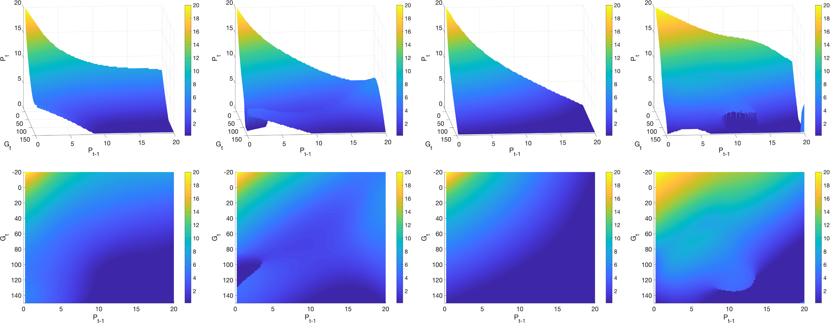
The starting state is selected uniformly at random from $\mathcal S$ . Furthermore, since discounting will lead to rewards after a large number of steps having a very limited effect on the total reward, we run each episode for at most 100 steps, before resetting to a starting state, again selected uniformly at random from $\mathcal S$ . This has the benefit of diversifying the states experienced, enabling us to achieve an approximate policy that is closer to the policy derived with dynamic programming as seen over the whole state space. The step size parameter used is

(5.2) \begin{align} \alpha_t = \min\!\left\{\alpha_0,\frac{1}{t^{0.5+\theta}}\right\},\end{align}

where $\alpha_t$ is the step size parameter used during episode t, and $0<\theta\leq0.5$ . The largest $\alpha_0$ that ensures that the weights do not explode can be found via trial and error. However, the value of $\alpha_0$ obtained in this way coincides with the “rule of thumb” for setting the step size parameter suggested in Sutton and Barto (Reference Sutton and Barto2018, Ch. 9.6), namely

\begin{align*}\alpha_0 = \frac{1}{\operatorname{E}_{\pi}\left[x^\top x\right]}, \quad \operatorname{E}_{\pi}\left[x^\top x\right] = \sum_{s,a}\mu_{\pi}(s)\pi(a|s) x(s,a)^\top x(s,a).\end{align*}

If $x\!\left(S_t,A_t\right)^\top x\!\left(S_t,A_t\right)\approx \operatorname{E}_{\pi}\left[x^\top x\right]$ , then this step size ensures that the error (i.e., the difference between the updated estimate $w_{t+1}^\top x\!\left(S_t,A_t\right)$ and the target $R_{t+1}+\gamma w_t^\top x(S_{t+1},A_{t+1}))$ is reduced to zero after one update. Hence, using a step size larger than $\alpha_0=\left(\operatorname{E}_{\pi}\left[x^\top x\right]\right)^{-1}$ risks overshooting the optimum, or even divergence of the algorithm. When using the Fourier basis of order n, this becomes for the examples studied here

\begin{align*}\operatorname{E}_{\pi}\left[x^\top x\right] &= \sum_{s,a}\mu_{\pi}(s)\pi(a|s)\sum_{i=1}^{(n+1)^{k+1}}\cos^2\Big(\pi(sc_{1:k}^{(i)}+ac_{k+1}^{(i)})\Big)\approx \frac{(n+1)^{k+1}}{2}.\end{align*}

For the simple model, we have used $\alpha_0 = 0.2$ for $n=1$ , $\alpha_0=0.07$ for $n=2$ , and $\alpha_0=0.03$ for $n=3$ . For the intermediate model, we used $\alpha_0 = 0.06$ for $n=1$ , $\alpha_0=0.008$ for $n=2$ , and $\alpha_0=0.002$ for $n=3$ . For the realistic model, we have used $\alpha_0=0.002$ for $n=3$ . In all cases $\alpha_0\approx \left(\operatorname{E}_{\pi}\left[x^\top x\right] \right)^{-1}$ . For $\theta,$ we tried values in the set $\{0.001,0.1,0.2,0.3,0.4,0.5\}$ . For the simple model, the best results were obtained with $\theta = 0.001$ irrespective of n. For the intermediate model, we used $\theta=0.5$ for $n=1$ , $\theta=0.2$ for $n=2$ , and $\theta=0.3$ for $n=3$ . For the realistic model, we used $\theta=0.2$ for $n=3$ .

Remark 5.3 (Step size). There are automatic methods for adapting the step size. One such method is the Autostep method from Mahmood et al. (Reference Mahmood, Sutton and Degris2012), a tuning-free version of the Incremental Delta-Bar-Delta (IDBD) algorithm from Sutton (Reference Sutton1992). When using this method, with parameters set as suggested by Mahmood et al. (Reference Mahmood, Sutton and Degris2012), the algorithm performs marginally worse compared to the results below.

Figure 2 shows the optimal policy for the simple model with terminal state using linear function approximation with 3rd-, 2nd-, and 1st-order Fourier basis using a softmax policy, and with 3rd-order Fourier basis using an $\varepsilon$ -greedy policy. Figure 1 shows that the approximate optimal policy using 3rd-order Fourier basis is close to the optimal policy derived with policy iteration. Using 1st- or 2nd-order Fourier basis also gives a reasonable approximation of the optimal policy, but worse performance. Combining 3rd-order Fourier basis and an $\varepsilon$ -greedy policy gives considerably worse performance.

The same conclusions can be drawn from Table 2, where we see the expected total discounted reward per episode for these policies, together with the results for the optimal policy derived with policy iteration, the policy derived with Q-learning, and several benchmark policies (see Section 5.1.3). Clearly, the performance of 3rd-order Fourier basis is very close to the performance of the optimal policy derived with policy iteration, and hence, we conclude that the linear function approximation with 3rd-order Fourier basis using a softmax policy appears to converge to approximately the optimal policy. The policy derived with Q-learning shows worse performance than both the 3rd- and 2nd-order Fourier basis, while the number of episodes run for the Q-learning algorithm is approximately a factor 30 bigger than the number of episodes run before convergence of SARSA with linear function approximation. Hence, even for this simple model, the number of states is too large for the Q-learning algorithm to converge within a reasonable amount of time. Furthermore, we see that all policies derived with linear function approximation using a softmax policy outperform the benchmark policies. Note that the optimal policy derived with policy iteration, the best constant policy, and the myopic policy with the terminal state require full knowledge of the underlying model and the transition probabilities, and the myopic policy with the constraint requires an estimate of the expected surplus one time step ahead, while the policies derived with function approximation or Q-learning only require real or simulated experience of the environment.

Table 2.

Expected discounted total reward (uniformly distributed starting states) for simple model with terminal state. The right column shows the fraction of episodes that end in the terminal state, within 100 time steps.

To analyse the difference between some of the policies, we simulate 300 episodes for the policy with the 3rd-order Fourier basis, the best constant policy, and the myopic policy with terminal state, $p_{\min}=5.8$ , for a few different starting states, two of which can be seen in Figure 3. A star in the figure corresponds to one or more terminations. The total number of terminations (of 300 episodes) are as follows: $S_0=({-}10,2)$ : Fourier 3:1, best constant: 291, myopic $p_{\min}=5.8$ : 20. $S_0=(50,7)$ : Fourier 3: 1, best constant: 0, myopic $p_{\min}=5.8$ : 20. For other starting states, the comparison is similar to that in Figure 3. We see that the policy with the 3rd order Fourier basis appears to outperform the myopic policy in all respects, that is on average the premium is lower, the premium is more stable over time, and we have very few defaults. The best constant policy naturally is the most stable, but leads to in general a higher premium compared to the other policies, and will for more strained starting states quickly lead to a large number of terminations.

Figure 3.

Simple model. Top row: policy with 3rd order Fourier basis. Bottom row: myopic policy with terminal state, $p_{\min}=5.8$ . Left: starting state $S_0=({-}10,2)$ . Right: starting state $S_0=(50,7)$ . The red line shows the best constant policy. A star indicates at least one termination.

5.1.3. Benchmark policies

Best constant policy. The best constant policy is the solution to

\begin{align*}\underset{p}{\text{minimise }}&\operatorname{E} \!\left[\sum_{t=0}^T \gamma^t h\!\left(p,S_{t+1}\right)\right].\end{align*}

For both the simple and intermediate models, $p=7.4$ solves this optimisation problem. For details, see the Supplemental Material, Section 4.1.

Myopic policy for MDP with constraint. The myopic policy maximises immediate rewards. For the model with a constraint on the action space, the myopic policy solves

(5.3) \begin{align} \underset{p}{\text{minimise }} c(p)\quad\text{subject to } \operatorname{E}\!\left[G_{1}\mid S_0=s,P_0=p\right]\geq 0.\end{align}

The myopic policy is given by the lowest premium level that satisfies the constraint. For details on how (5.3) is solved, see the Supplemental Material, Section 4.2.

For the simple, intermediate, and realistic model, the myopic policy charges the minimum premium level for a large number of states. Since this policy so quickly reduces the premium to the minimum level as the surplus or previously charged premium increases, it is not likely to work that well. Hence, we suggest an additional benchmark policy where we set the minimum premium level to a higher value, $p_{\min}$ . Thus, this adjusted myopic policy is given by $\tilde \pi(s) = \max\{\pi(s),p_{\min}\}$ , where $\pi$ denotes the policy that solves (5.3). Based on simulations of the total expected discounted reward per episode for different values of $p_{\min}$ , we conclude that $p_{\min}=6.4$ achieves the best results for both the simple and intermediate model, and $p_{\min}=10.5$ achieves the best result for the realistic model.

Myopic policy for MDP with terminal state. For the model with a terminal state, the myopic policy is the solution to the optimisation problem

(5.4) \begin{align} \underset{p}{\text{minimise }} &\operatorname{E} \!\left[h(p,S_{1})\mid S_0=s,P_0=p\right].\end{align}

For details on how (5.4) is solved, see the Supplemental Material, Section 4.3. We also suggest an additional benchmark policy where the minimum premium level has been set to $p_{\min}=5.8$ , the level that achieves the best results based on simulations of the total expected discounted reward per episode. For the intermediate and realistic model, this myopic policy is too complex and is therefore not a good benchmark.

5.2. Intermediate model

We use the following parameter values: $\gamma=0.9$ , $\mu=5$ , $\beta_0=10$ , $\beta_1=1$ , $\xi=0.05$ , $\nu=1$ , $\alpha_1=0.7$ , $\alpha_2=0.3$ , $\eta=10$ , $a=18$ , $b=-0.3$ , and cost function (5.1) with $c_1=1$ and $c_2=1.2$ . The premium level and number of contracts written are truncated and discretised according to $\mathcal A = \{0.2,0.4,\ldots,19.8,20.0\}$ and $\mathcal N = \{0,1,\ldots,30\}$ . The surplus process no longer only takes integer values (as in the simple model), instead the values that the surplus process can take are determined by the parameter values chosen. However, it is still truncated to lie between –20 and 150. For the parameter values above, we have $\mathcal G = \{-20.00,-19.95,\ldots,149.95,150.00\}$ .

Figure 4 shows the optimal policy for the intermediate model using linear function approximation, with 3rd-, 2nd-, and 1st-order Fourier basis, for $N_{t}=N_{t-1}=10$ . Comparing the policy with the 3rd-order Fourier basis with the policy with the 2nd order Fourier basis, the former appears to require a slightly lower premium when the surplus or previously charged premium is very low. The policy with the 1st-order Fourier basis appears quite extreme compared to the other two policies. Comparing the policy with the 3rd-order Fourier basis for $N_{t}=N_{t-1}=10$ with the optimal policy for the simple model (bottom row in Figure 1), we note that $\pi^{i}(g,p,10,10)\neq \pi^s(g,p)$ , where $\pi^s$ and $\pi^{i}$ denotes, respectively, the policy for the simple and the intermediate model. There is a qualitative difference between these policies, since even given that we are in a state where $N_t=N_{t-1}=10$ using the intermediate model, the policy from the simple model does not take into account the effect the premium charged will have on the number of contracts issued at time $t+1$ . The policy with 3rd-order Fourier basis for $N_t,N_{t-1}\in\{5,10,15\}$ can be seen in Figure 5.

Figure 4.

Optimal policy for intermediate model with terminal state using linear function approximation, $N_t=N_{t-1}=10$ . Left: 3rd-order Fourier basis. Middle: 2nd-order Fourier basis. Right: 1st-order Fourier basis.

Figure 5.

Optimal policy for the intermediate model with terminal state using linear function approximation with 3rd-order Fourier basis, for $N_t,N_{t-1}\in\{5,10,15\}$ .

To determine the performance of the policies for the intermediate model, we simulate the expected total discounted reward per episode for these policies. The results can be seen in Table 3. Here we clearly see that the policy with 3rd-order Fourier basis outperforms the other policies and that the policy with 1st-order Fourier basis performs quite badly since is not flexible enough to be used in this more realistic setting. We also compare the policies with the optimal policy derived with policy iteration from the simple model while simulating from the intermediate model. Though this policy performs worse compared to the policy with 3rd- and 2nd-order Fourier basis, it outperforms the policy with 1st-order Fourier basis. Note that the policies derived with function approximation only require real or simulated experience of the environment. The results for the myopic policy in Table 3 use the true parameters when computing the expected value of the surplus. Despite this, the policy derived with the 3rd order Fourier basis outperforms the myopic policy.

Table 3.

Expected discounted total reward based on simulation, (uniformly distributed starting states). The right column shows the fraction of episodes that end in the terminal state, within 100 time steps.

To analyse the difference between some of the policies, we simulate 300 episodes for the policy with the 3rd-order Fourier basis, the best constant policy and the policy from the simple model, for a few different starting states, two of which can be seen in Figure 6. Each star in the figures correspond to one or more terminations at that time point. The total number of terminations (of 300 episodes) are as follows: $S_0=(0, 7, 10, 10)$ : Fourier 3: 1, best constant: 13, simple: 5. $S_0=(100, 15, 5, 5)$ : Fourier 3: 0, best constant: 0, simple: 10. Comparing the policy with the 3rd-order Fourier basis with the policy from the simple model, we see that it tends to on average give a lower premium and leads to very few defaults, but is slightly more variable compared to the premium charged by the simple policy. This is not surprising, since the simple policy does not take the variation in the number of contracts issued into account. At the same time, this is to the detriment of the simple policy, since it cannot correctly take the risk of the varying number of contracts into account, hence leading to more defaults. For example, for the more strained starting state $S_0=({-}10,2,20,20)$ (not shown in figure), the number of defaults for the policy with the 3rd order Fourier basis is 91 of 300, and for the simple policy it is 213 of 300. Similarly, for starting state $S_0=(100, 15, 5, 5)$ (second column in Figure 6), the simple policy will tend set the premium much too low during the first time step, hence leading to more early defaults compared to for example starting state $S_0=(0, 7, 20, 20)$ (first column in Figure 6), despite the fact that the latter starting state has a much lower starting surplus.

Figure 6.

Intermediate model. Top row: policy with 3rd Fourier basis. Bottom row: policy from the simple model. Left: starting state $S_0=(0, 7, 20, 20)$ . Right: starting state $S_0=(100, 15, 5, 5)$ . The red line shows the best constant policy. A star indicates at least one termination.

5.3. Realistic model

To estimate the parameters of the model for the cumulative claims payments in (2.8), we use the motor third party liability data considered in Miranda et al. (Reference Miranda, Nielsen and Verrall2012). The data consist of incremental runoff triangles for number of reported accidents and incremental payments, with 10 development years. We have no information on the number of contracts. For parameter estimation only, we assume a constant number of contracts over the ten observed years, that is $\widetilde N_{t+1}=N$ , and that the total number of claims for each accident year is approximately 5% of the number of contracts. We further assume that the total number of claims per accident year is well approximated by the number of reported claims over the first two development years. This leads to an estimate of the number of contracts $\widetilde N_{t+1}$ in (2.8) of $\widehat N = 2.17\cdot 10^5$ . For parameter estimation, we assume that $\mu_{0,t}=\mu_0$ in (2.9). Hence, $\mu_0$ and $\nu_0^2$ are estimated as the sample mean and variance of $\left(\log\!\left(C_{t,1}\right)\right)_{t=1}^{10}$ . Similarly, $\mu_j$ and $\nu_j^2$ are estimated as the sample mean and variance of $\left(\log\!\left(C_{t,j+1}/C_{t,j}\right)\right)_{t=1}^{10-j}$ for $j=1,\ldots,8$ . Since we only have one observation for $j=9$ , we let $\widehat \mu_9=\log\!\left(C_{1,10}/C_{1,9}\right)$ and $\widehat \nu_9=0$ . $c_0$ is estimated by $\widehat c_0 = \exp\!\left\{\widehat \mu_0+\widehat \nu_0^2/2\right\}/\widehat N\approx 2.64$ . The parameter estimates can be seen in Table 1 in the Supplemental Material, Section 5.

For the model for investment earnings, the parameters are set to $\widetilde \sigma=0.03$ and $\widetilde \mu = \log(1.05)-\widetilde\sigma^2/2$ , which gives similar variation in investment earnings as in the intermediate model (2.7) when the surplus is approximately 50. The remaining parameters are $\gamma=0.9$ , $\beta_0=2\cdot 10^5$ , $\beta_1=1$ , $\eta=10$ , and $b=-0.3$ . The parameter a is set so that the expected number of contracts is $2\cdot 10^5$ when the premium level corresponds to the expected total cost per contract, $\beta_0/(2\cdot10^5)+\beta_1+c_0/\alpha_1 \approx 10.4$ . Hence, $a\approx 4.03\cdot 10^5$ . The premium level is truncated and discretised according to $\mathcal A = \{0.5,1.0,\ldots,29.5,30.0\}$ The cost function is as before (5.1), but now adjusted to give rewards of similar size as in the simple and intermediate setting. Hence, when computing the reward, the premium is adjusted to lie in $[0.2,20.0]$ according to

\begin{align*}c(p)=\widetilde p +c_1\left(c_2^{\widetilde p}-1\right),\quad \text{where }\widetilde p = 0.2 + \frac{p-0.5}{30-0.5}(20-0.2).\end{align*}

The number of contracts is truncated according to $\mathcal N= \{144170, \ldots, 498601\}$ . This is based on the $0.001$ -quantile of $\textsf{Pois}(a(\!\max\mathcal A)^b)$ , and the $0.999$ -quantile of $\textsf{Pois}(a(\min\mathcal A)^b)$ . The truncation of the cumulative claims payments $C_{t,j}$ is based on the same quantile levels and lognormal distributions with parameters $\mu=\log(c_0\min\mathcal N)-\nu_0^2/2+\sum_{k=1}^{j-1}\mu_k$ and $\sigma^2 = \sum_{k=0}^{j-1}\nu_k$ , and with parameters $\mu=\log(c_0\max\mathcal N)-\nu_0^2/2+\sum_{k=1}^{j-1}\mu_k$ and $\sigma^2 = \sum_{k=0}^{j-1}\nu_k$ , respectively, for $j=1,\ldots,9$ . The truncation for the cumulative claims payments can be seen in Table 2 in the Supplemental Material, Section 5. The surplus is truncated to lie in $[{-}0.6,4.5]\cdot 10^6$ . Note that for the realistic model, with 10 development years the state space becomes 13-dimensional. Using the full 3rd-order Fourier basis is not possible since it consists of $4^{14}$ basis functions. We reduce the number of basis functions allowing for more flexibility where the model is likely to need it. Specifically,

\begin{align*}&\left\{\left(c^{(i)}_1,c^{(i)}_2,c^{(i)}_3,c^{(i)}_4,c^{(i)}_{14}\right)\,:\,i=1,\dots,4^5\right\}=\{0,\dots,3\}^5, \\[4pt]&c^{(i)}_1=c^{(i)}_2=c^{(i)}_3=c^{(i)}_4=c^{(i)}_{14}=0 \quad \text{for } i=4^5+1,\dots,4^5+9,\end{align*}

and, for $j=1,\ldots,9$ ,

\begin{align*}c^{(i)}_{4+j}=\left\{\begin{array}{ll}1 & \text{for } i=4^5 + j, \\[5pt]0 & \text{for } i\neq 4^5+j.\end{array}\right.\end{align*}

This means less flexibility for variables corresponding to the cumulative payments and no interaction terms between a variable corresponding to a cumulative payment and any other variable.

Figure 7 shows the optimal policy for the realistic model using linear function approximation for $N_t,N_{t-1}\in\{1.75,2.00,2.50\}\cdot 10^5$ , $C_{t-1,1} = c_0\cdot2\cdot 10^5$ , and $C_{t-j,j} = c_0\cdot2\cdot 10^5\prod_{k=1}^{j-1}f_k$ for $j=2,\ldots,9$ . To determine the performance of the approximate optimal policy for the realistic model, we simulate the expected total discounted reward per episode for this policy. The results can be seen in Table 4. The approximate optimal policy outperforms all benchmark policies. The best performing benchmark policy, the “interval policy,” corresponds to choosing the premium level to be equal to the expected total cost per contract, when the number of contracts is $2\cdot 10^5$ , as long as the surplus lies in the interval $[1.2,2.8]\cdot 10^6$ . This is based on a target surplus of $2\cdot 10^6$ and choosing $\phi\in\{0.1,0.2,\ldots,1.0\}$ that results in the best expected total reward, where the interval for the surplus is given by $[1-\phi,1+\phi]\cdot 2\cdot 10^6$ . When the surplus $G_t$ is below (above) this interval, the premium is increased (decreased) in order to decrease (increase) the surplus. The premium for this benchmark policy is

\begin{align*}P_t =\begin{cases}\min\!\left\{10.5+\dfrac{(1-\phi)\cdot2\cdot10^6-G_t}{2\cdot10^5},\max\mathcal A\right\},\quad &\text{if } G_t<(1-\phi)\cdot2\cdot10^6,\\[9pt] 10.5, \quad & \text{if } (1-\phi)\cdot2\cdot10^6\leq G_t\leq (1+\phi)\cdot2\cdot10^6,\\[9pt] \max\!\left\{10.5+\dfrac{(1+\phi)\cdot2\cdot10^6-G_t}{2\cdot10^5},\min\mathcal A\right\},\quad &\text{if } (1+\phi)\cdot2\cdot10^6<G_t,\end{cases}\end{align*}

and rounded to the nearest half integer, to lie in $\mathcal A$ . As before the approximate optimal policy outperforms the benchmark policies despite the fact that both the myopic and the interval policy use the true parameters when computing the expected surplus or the expected total cost per contract.

Figure 7.

Optimal policy for realistic model with terminal state using linear function approximation, for $N_t,N_{t-1}\in\{1.75, 2.00, 2.50\}\cdot10^5$ , $C_{t-1,1} = c_0\cdot2\cdot 10^5$ , and $C_{t-j,j} = c_0\cdot2\cdot 10^5\prod_{k=1}^{j-1}f_k$ .

Table 4.

Expected discounted total reward based on simulation, (uniformly distributed starting states). The right column shows the fraction of episodes that end in the terminal state, within 100 time steps.

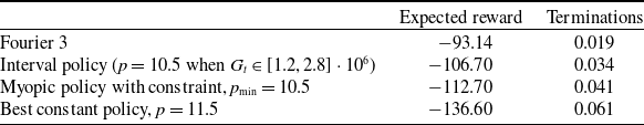
A comparison of the approximate optimal policy and the best benchmark policy, including a figure similar to Figure 6, is found in the Supplemental Material, Section 5.