

INTRODUCTION
Maize is one of the three key crops around the globe in terms of production and as a dietary staple (Nuss & Tanumihardjo Reference Nuss and Tanumihardjo2010). Mexico, its centre of origin and diversification (Kato et al. Reference Kato, Mapes, Mera, Serratos and Bye2009), harbours around 59 native races and thousands of local varieties (created through natural and human selection over thousands of years), representing the most important genetic reservoir for this species in the world (Ruiz Corral et al. Reference Ruiz Corral, Durán Puga, Sánchez Gonzáles, Ron Parra, González Euiarte, Holland and Medina García2008) and the basis of Mexican culture and cuisine (Barros & Buenrostro Reference Barros and Buenrostro2011). Although the taxonomic term ‘race’ is not commonly used in agricultural plants, in the case of maize it has been very useful to assist with organizing the species’ great diversity (Anderson & Cutler Reference Anderson and Cutler1942). A well-accepted definition of race is as follows: ‘a group of related individuals with enough characteristics in common to permit their recognition as a group’ (Anderson & Cutler Reference Anderson and Cutler1942). Some Mexican maize experts suggest that since there is a continuous genetic flow between maize populations, they are not isolated enough to create sub-species and consequently it is better to classify them as races (Ortega Paczka, personal communication). It is also known that within each race a wide range of variants exists (Rocandio-Rodríguez et al. Reference Rocandio-Rodríguez, Santacruz-Varela, Córdova-Téllez, López-Sánchez, Castillo-González, Lobato-Ortiz and García-Zavala2014).
In Mexico, c. 0·85 of farmers growing maize are smallholders (<5 ha producing 1·6–2 t/ha) (Cruz Delgado et al. Reference Cruz Delgado, Gómez Valdez, Ortiz Pulido, Entzana Tadeo, Suárez Hernández and Santillán Moctezuma2012) who grow mostly native races using open-pollinated populations of traditional ‘owned’ seed stocks and agro-technologies, with yields depending strongly on environmental conditions (Turrent Fernández Reference Turrent Fernández, Rodríguez Montessoro and de Léon2008). Yield depends on the biological characteristics of the race, such as cycle length (Chávez-Servia et al. Reference Chávez-Servia, Tuxill and Jarvis2004), but each race presents a wide range of yield variation across the race distribution, thus exhibiting plasticity depending on a range of environmental growth conditions (Acevedo et al. Reference Acevedo, Huerta, Burgeff, Koleff and Sarukhán2011; CONABIO 2011).
In recent years, some efforts have been focused on modelling geographic patterns of fitness using presence-only data for wild species (VanDerWal et al. Reference VanDerWal, Shoo, Johnson and Williams2009; Tôrres et al. Reference Tôrres, De Marco Júnior, Santos, Silveira, de Almeida Jácomo and Diniz-Filho2012; Yañez-Arenas et al. Reference Yañez-Arenas, Martínez-Meyer, Mandujano and Rojas-Soto2012, Reference Yañez-Arenas, Peterson, Mokondoko, Rojas-Soto and Martínez-Meyer2014; Martínez-Meyer et al. Reference Martínez-Meyer, Díaz-Porras, Peterson and Yañez-Arenas2013; Nagaraju et al. Reference Nagaraju, Gudasalamani, Barve, Ghazoul, Narayanagowda and Ramanan2013; Lira-Noriega & Manthey Reference Lira-Noriega and Manthey2014). A study carried out in India with the economically important tree Myristica malabarica showed that highly suitable sites projected with ecological niche modelling were correlated significantly with higher plant fitness. To evaluate fitness, Nagaraju et al. (Reference Nagaraju, Gudasalamani, Barve, Ghazoul, Narayanagowda and Ramanan2013) evaluated functional traits of the plant, such as fluctuating asymmetry, leaf weight, recruitment and genetic variability. Other studies have tested whether ecological niche modelling outcomes are related to the abundance (as an expression of fitness) of several species, resulting in marginal success in the best cases (VanDerWal et al. Reference VanDerWal, Shoo, Johnson and Williams2009; Tôrres et al. Reference Tôrres, De Marco Júnior, Santos, Silveira, de Almeida Jácomo and Diniz-Filho2012). On the other hand, a novel method to model geographic patterns of abundance based on the ecological niche theory, named the Distance to the Niche Centroid approach, was proposed and tested by Martínez-Meyer et al. (Reference Martínez-Meyer, Díaz-Porras, Peterson and Yañez-Arenas2013), and implemented by Yañez-Arenas et al. (Reference Yañez-Arenas, Martínez-Meyer, Mandujano and Rojas-Soto2012). According to Maguire (Reference Maguire1973), population fitness should be maximal where the highest birth rate and the lowest death rate coincide in the multi-dimensional niche space; he proposed that such optimal conditions should occur at or near the centroid of the niche hypervolume for each species. Based on this body of theory, Martínez-Meyer et al. (Reference Martínez-Meyer, Díaz-Porras, Peterson and Yañez-Arenas2013) successfully tested the hypothesis that population abundances of 11 species of vertebrates follow a centre-abundant pattern in ecological space, where maximal abundance occurs around the niche centroid (NC) and decreases progressively as populations depart from this point. An implementation of this procedure for the white-tailed deer (Odocoileus virginianus) produced robust spatially explicit models of abundance in two regions of Mexico (Yañez-Arenas et al. Reference Yañez-Arenas, Martínez-Meyer, Mandujano and Rojas-Soto2012). Other studies have already incorporated this concept to infer potential risk areas for snakebite (Yañez-Arenas et al. Reference Yañez-Arenas, Peterson, Mokondoko, Rojas-Soto and Martínez-Meyer2014) and to test whether there was a relationship between genetic diversity and distance to the NC (Lira-Noriega & Manthey Reference Lira-Noriega and Manthey2014). However; it is theoretically feasible that optimum conditions for a given species are not always at or near the central values of specific critical ecological variables (i.e. NC); for example, some monkeyflower species have higher fitness at their marginal elevation range (Angert Reference Angert2009). Consequently, the niche optimum (NO) may be off the centre of the niche hypervolume.
Following this line of thinking, it was hypothesized that Mexican maize races will exhibit higher yields in areas that are ecologically closer to the optimum of their ecological niches (NO), which may or may not coincide with their centroids (NC). Even when yield does not necessarily reflect higher fitness for the plant (as it has been selected to cover human needs and not to reach its own ‘biological success’), both natural and human selection have operated under specific environmental conditions and one of the key traits targeted in the latter is yield (Herrera-Cabrera et al. Reference Herrera-Cabrera, Castillo-González, Sánchez-González, Hernández-Casillas, Ortega-Paczka and Goodman2004; Yamasaki et al. Reference Yamasaki, Tenaillon, Vroh Bi, Schroeder, Sanchez-Villeda, Doebley, Gaut and McMullen2005). Today, each race is distributed across a range of environmental conditions, which may be considered equivalent to its ecological niche (Ruiz Corral et al. Reference Ruiz Corral, Durán Puga, Sánchez Gonzáles, Ron Parra, González Euiarte, Holland and Medina García2008; Ureta et al. Reference Ureta, Martínez-Meyer, Perales and Álvarez-Buylla2012; Ruiz Corral et al. Reference Ruiz Corral, Sánchez González, Hernández Casillas, Willcox, Ramírez Ojeda, Ramírez Díaz and González Eguiarte2013) and where it should be possible to find an NC/NO. Furthermore, higher yields have already been documented for cereals (such as maize, wheat and oats) under specific optimum environmental conditions for the plant (Boyer Reference Boyer1982).
The present study tested whether there was a relationship between yield and the distance to the NC/NO of nine different local Mexican maize races for which sufficient and relatively well-distributed yield data across their geographic range were found. Additionally, geographically and environmentally homogeneous clusters were identified for each race studied and the same analyses carried out to evaluate whether different NOs may exist in one single race. Finally, the yields of races Celaya, Vandeño and Tepecintle were projected under current and future climate change conditions (2050) at the race level, as well as the clusters with higher fitness for Celaya and Vandeño. The information generated in the present study may aid in identifying which factors are critical for yield in maize races. Thus, in turn, this may help with searching for new areas of production for a particular race that mimic their current optimal yield conditions, or may contribute with variables and models to estimate future yields under different conditions and in different geographical areas. If it is possible to demonstrate that this method works with domesticated plants under traditional management, then it is a step forward in conservation planning for key food and genetic resources in the face of environmental change.
METHODS
Occurrence and yield data
Occurrence records from 1980 to 2010 (Acevedo et al. Reference Acevedo, Huerta, Burgeff, Koleff and Sarukhán2011) and yield information from 2000 to 2010 were obtained from a database compiled by the Mexican Commission for Biodiversity (CONABIO 2011). The yield information was taken from a column named ‘rendimiento uniformizada1’: as indicated by the document accompanying this database, this column takes into account all information that was taken from the field and was assigned a single numerical number in kg/ha units (in cases where the information constituted intervals or some other kind of measurement, it was transformed into the corresponding units to unify quantities and make them comparable). For some localities two types of data could be found: uniformizada1 and uniformizada2, representing two different seasons (spring/summer and autumn/winter). The column uniformizada1 was the only one taken into account in the present study, since this is the season in which >0·80 of Mexican maize is produced. At present, there is no official institution gathering exact estimates of native race yields, so farmers were interviewed and provided an approximate value of their annual productivity. However, the method proposed in the present study is expected to work even if approximate yield data is available. Consequently, interviews might still give valuable information at a race level that can provide an idea of the yield magnitudes and variation along their distribution ranges, under current and future conditions. Furthermore, it was decided to take out statistical outliers (mean ± 2sd) that made no biological or agronomic sense. For example, race Bolita presents an average yield of 2·5 t/ha, but two values out of 35 were >8 t/ha. These two values are obviously statistical outliers as yields above 8 t/ha would only be expected in the high production areas of hybrid maize varieties using modern agro-technology, such as irrigation, fertilizers and pesticides (Cruz Delgado et al. Reference Cruz Delgado, Gómez Valdez, Ortiz Pulido, Entzana Tadeo, Suárez Hernández and Santillán Moctezuma2012). Using this procedure no more than three records per race were discarded (one for Celaya out of 86, one for Cónico Norteño out of 235, three for Tabloncillo out of 63, and three for Tuxpeño out of 534; for the remaining five races all records were taken into account for the analysis). The races analysed were: Bolita, Celaya, Cónico Norteño, Olotillo, Ratón, Tabloncillo, Tepecintle, Tuxpeño y Vandeño (Table 1). To characterize the bioclimatic profile of these races a 1 km2 resolution climatology map generated for Mexico covering 1980–2009 was used (Cuervo-Robayo Reference Cuervo-Robayo2014).
Linear models describing the relationship between yield and distance to the ecological niche centroid/optimum for nine maize races
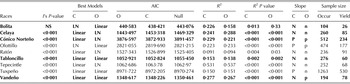
NS, not significant.
I's P value: P value of the Moran's I test on spatial autocorrelation (H 0: no spatial autocorrelation exists), Best model: best of two models; Linear: Yield = β 0 + β 1 × Distance, LN: Yield = β 0 + β 1 × ln (Distance), C: centroid, O: optimum, AIC: Akaike Information Criterion of the best model, bold: highlights a model with a smaller AIC than the one of the null model (Yield = β 0), R 2: coefficient of determination associated to the best model, R 2 P value: R 2 significance P value, Slope: sign of the value of the β 1 estimate of the best model (n, negative; p, positive), Sample size: number of occurrence and yield data.
Calculating distances to ecological centroids and optima
For all data relating to presence, the value for each of the 19 bioclimatic variables evaluated was obtained (1: annual mean temperature, 2: mean diurnal range, 3: isothermality, 4: temperature seasonality, 5: maximum temperature of the warmest month, 6: minimum temperature of the coldest month, 7: temperature annual range, 8: mean temperature of the wettest quarter, 9: mean temperature of the driest quarter, 10: mean temperature of the warmest quarter, 11: mean temperature of the coldest quarter, 12: annual precipitation, 13: precipitation of the wettest month, 14: precipitation of the driest month, 15: precipitation seasonality, 16: precipitation of the wettest quarter, 17: precipitation of the driest quarter, 18: precipitation of the warmest quarter and 19: precipitation of the coldest quarter). All these variables were included even though the races are mostly grown during the spring–summer season, because it has been shown that climatic variables at other times of the year are still significantly related to the distribution of most races (Ureta et al. Reference Ureta, González-Salazar, González, Álvarez-Buylla and Martínez-Meyer2013). The ecological niche modelling program MaxEnt (Phillips et al. Reference Phillips, Anderson and Schapire2006) was then used to identify which variables contributed most to the distribution of each race and these were used for the correlation analysis between the yield and distance to NC and NO. Only bioclimatic variables were used in the present study because the aim was to project the effect of climate change on the distribution of future yield, but it should be noted that other environmental factors (e.g. soil and slope) are also important for characterizing the niche of a species such as maize (Ureta et al. Reference Ureta, González-Salazar, González, Álvarez-Buylla and Martínez-Meyer2013; Dyer et al. Reference Dyer, López-Feldman, Yúnez-Naude and Taylor2014).
Once the bioclimatic variables were associated with the presence data, distances were calculated to the NC (Yañez-Arenas et al. Reference Yañez-Arenas, Martínez-Meyer, Mandujano and Rojas-Soto2012; Martínez-Meyer et al. Reference Martínez-Meyer, Díaz-Porras, Peterson and Yañez-Arenas2013) and NO. The NC was calculated as the standardized mean assuming a normal distribution of the range of each bioclimatic variable where the race was present. Although ecological theory suggests that higher suitability and consequently higher fitness should be found in the NC (Maguire Reference Maguire1973), it may be the case that the optimal conditions do not coincide with the centroid because a species may be adapted to extreme (or at least off-centre) conditions for a given environmental variable (Angert Reference Angert2009). Therefore, the Euclidian distance was measured to a multi-dimensional point, the NO. To calculate NO, a function for building the response curves of the maize race presence records with respect to each environmental variable was used and implemented in MaxEnt, which identified the value of each environmental variable for which the presence response for that taxon was most frequent. To run MaxEnt, 0·70 of the dataset was used for training the model and the remaining 0·30 to test it. Validation of the model was performed with a partial-receiver operating characteristic (ROC) test (Peterson et al. Reference Peterson, Papeş and Soberón2008), which has the advantage of taking into account only the projected area when using the niche algorithm and does not evaluate omissions and commissions (i.e. false positive errors in Ecological Niche Modeling) equally (Peterson et al. Reference Peterson, Soberón, Pearson, Anderson, Mazrtínez-Meyer, Nakamura and Araújo2011). Omissions should be punished harder. Once the NC and NO values were identified, all bioclimatic variables were z-standardized, thus the NC (multivariate mean) was zero. Then, the multidimensional Euclidian distance of every occurrence record to the NC and the NO was calculated. Thus, the distance (d) of the data point P i to the niche (N = NC or NO) is:
 $$\hskip -9pc d({P_i}\comma N) = {({S_j}{({P_{i\comma j}}-{N_j})^2})^{1/2}}$$
where P i,j and N j are the values of the jth bioclimatic variable of the data point P i and NC or NO, respectively. The calculation of the Euclidian distance to NC or NO was done for every race record under current climatic conditions. However; under future climatic conditions the potential distribution area was necessary; consequently, the calculation of the Euclidian distance was done for every 10 km2 (the resolution of the climate change map), to show where the race was modelled to be distributed in the future (see below).
Relationship between yield and distance to ecological centroids and optima
Once the distance to the NC and NO were obtained for every presence datum point, those occurrences for which yield data were available were taken to model the relationship between yield and distance to the NC/NO. Since spatial autocorrelation existed among the data for each race (using the Moran's I test, Table 1) (Fortin & Dale Reference Fortin and Dale2005), three autoregressive models were fitted:
-
(a) Yield = β 0,
-
(b) Yield = β 0 + β 1 × Distance, and
-
(c) Yield = β 0 + β 1 × ln (Distance).
For those cases where the Moran's I test showed existing autocorrelation, a conditional autoregressive model was used to deal with univariate models (Gelfand & Vounatsou Reference Gelfand and Vounatsou2003); and the spdep package in R was used to fit these models (Bivand et al. Reference Bivand, Altman, Anselin, Assunçáo, Berke, Bernat, Blanchet, Blankmeyer, Carvalho, Christensen, Chun, Dormann, Dray, Gómez-Rubio, Halbersma, Krainski, Legendre, Lewin-Koh, Li, Ma, Millo, Mueller, Ono, Peres-Neto, Piras, Reder, Tiefelsdorf and Yu2014; R Development Core Team 2014). The Akaike Information Criterion (AIC, Akaike Reference Akaike1974) and determination coefficient (R 2) were calculated to perform model selection and evaluate model fitting, respectively. It was also evaluated if differences could be found between models using the distance to the NC and to the NO.
Potential distribution maps under current and future climatic conditions
Most races evaluated are distributed widely throughout Mexico, encompassing different climates. Consequently, data were split into environmental and geographic clusters. These clusters were created through the ‘partitioning around medoids’ clustering algorithm. This algorithm has the advantage of not requiring an a priori fixed number of clusters. The environmental clustering was performed with 13 of the 19 bioclimatic variables (1, 5, 6, 8, 9, 10, 11, 12, 13, 16, 17, 18 and 19) because these showed low correlations among them and with the others. The algorithm was implemented through the fpc package in R (Hennig Reference Hennig2010; Pinheiro et al. Reference Pinheiro, Bates, DebRoy and Sarkar2011). The environmental clustering helped to identify sub-groups with similar ecological profiles, while geographic clustering identified sub-groups that, due to their geographic closeness, are expected to be genetically similar. It was decided to create clusters because there is evidence supporting an important ecological and genetic variation within races. If clusters improve correlations between yield and distance to the NC or NO, it indicates that there is more than one NC or NO within a race and there is an important amount of yield variation (Herrera-Cabrera et al. Reference Herrera-Cabrera, Castillo-González, Sánchez-González, Hernández-Casillas, Ortega-Paczka and Goodman2004).
To project occurrences of higher yields under current and future climatic conditions, three races were chosen based on their AIC and R 2 values: Celaya, Vandeño and Tepecintle. An environmental cluster for Celaya (Celaya 3) and a geographic cluster for Vandeño (Vandeño 2) were also projected. No cluster was projected for Tepecintle because the proportion of explained deviance was greater at the race level than with any cluster. For the current climate conditions (1980–2011), the same climatology as above was used, and for the future (2040–2069, hereafter called 2050), climatologies drawn from the Moscow Forestry Sciences Laboratory (http://forest.moscowfsl.wsu.edu/climate/) were used. The general circulation model (GCM) used was the Hadley Centre Global Environmental Model version 1 (HadGEM1), developed in the UK: this has been evaluated by Mexican climatologists as one of the best in representing Mexico's current climate and thus produces reasonable future climatic scenarios (Conde Álvares & Gay Garciá Reference Conde Álvares and Gay Garciá2008). The worst case emission scenario A2 (‘business as usual’) was assessed (IPCC Reference Solomon, Qin, Manning, Chen, Marquis, Averty, Tignor and Miller2007). Although there is awareness of the new scenarios proposed by the IPCC, ‘Representative Concentration Pathways’ (IPCC Reference Field, Barros, Dokken, Mach, Mastrandrea, Bilir, Chatterjee, Ebi, Estrada, Genova, Girma, Kissel, Levy, MacCracken, Mastrandrea and White2014), it was decided not to use these models, because they have not been downscaled specifically for Mexico to a 1 km2 resolution. Until now, Mexican government downscaling efforts (10 km2) have taken place through the Reliability Ensemble Averaging method, that takes into account all General Circulation Models giving higher weight to those performing better in specific areas of the country (Ibarra-Cardeña et al. Reference Ibarra-Cardeña, Cavazos, Salinas, Martínez, Colorado, De Grau, Prieto González, Conde Álvarez, Quintanar, Santana Sepúlveda, Romero Centeno, Maya Magaña, Rosario de La Cruz, Ayala Enríquez, Carrillo Tlazazanatza, Santiesteban and Bravo2013).
Current climatology was generated for Mexico using the thin-plate spline technique available in the ANUCLIM program (http://fennerschool.anu.edu.au) at 1 km2 spatial resolution (Cuervo-Robayo Reference Cuervo-Robayo2014). Under current climatic conditions, the potential distribution area was modelled with the only purpose of calculating the proportion of potential distribution area that would be lost in the future. The distance to NC/NO was calculated only with present data as explained above.
To locate future possible regions of higher yields, firstly future potential distribution areas were modelled by running ten model replicates for each emission scenario with the MaxEnt algorithm (Phillips et al. Reference Phillips, Anderson and Schapire2006). Replicate probability output was then converted into a binary map using the maximal threshold value that minimized the training and test omission rate. As a way to reduce uncertainty, binary maps were assembled and the final map was the consensus of all ten maps (Araújo & New Reference Araújo and New2007). A final map was combined with the 19 bioclimatic variables obtained for 2050 under the emission scenario A2. The bioclimatic profile for each pixel of the potential distribution area was obtained and the distance to the current NC or NO was calculated (assuming that these values will be maintained through time). In this way, the geographic areas with potentially higher yields in the future for the races Celaya, Vandeño, Tepecintle and the corresponding clusters were identified.
RESULTS
Relationship between yield and distance to ecological centroids and optima
The NO was identified via ecological niche modelling. All ecological niche models presented good performance as indicated by their high average Partial ROC: AUC ratios and P values that were always highly significant (P < 0·001) (see Table S1 in the Supplementary Material for details, available from http://journals.cambridge.org/AGS).
Moran's I tests performed on the data for each race showed that negative autocorrelation existed among the data and was statistically significant (P < 0·001) in eight of the nine races (Table 1). These negative autocorrelations persisted for all the ecological and geographic clusters (Tables S1 and S2, available from http://journals.cambridge.org/AGS). As expected, when geographic clustering was performed, autocorrelation within each of these clusters was lost more often than within ecological clusters.
At the race level, all showed a significant (P < 0·015) correlation between yield and the distance to NC and/or NO. However, the best models were selected over the null model (model a) in only six of the nine races: Bolita, Celaya, Cónico Norteño, Olotillo, Tabloncillo, Tepecintle and Vandeño (Table 1). From these six races, only Cónico Norteño presented a positive correlation with NC and NO (Table 1). Bolita, Celaya, Olotillo, Tepecintle and Vandeño presented negative correlations between yield and distance to both NC and to NO. For most of these races, R 2 values were higher when evaluating the distance to the NC than to the NO (Table 1). The exceptions were Celaya and Tepecintle, which were also the races presenting the highest R 2 values (0·288 and 0·537, respectively).
When carrying out the environmental cluster analysis, sub-groups for some races presented better models than the null model and higher proportions of explained deviance. For example, Celaya increased its R 2 up to 0·774 in one of its environmental clusters (Celaya 3) (Table 1, Table S2, available from http://journals.cambridge.org/AGS). In races that showed no significant correlations at the race level, such as Olotillo, Ratón and Tuxpeño, significant (P < 0·001) negative correlations were found with R 2 values of up to 0·298 in some of their sub-groups. With this clustering, it was possible to find five negative correlations and two positive ones. Higher yields for these environmental sub-groups were better explained by distance to the NO than by distance to the NC, except for Vandeño which presented only one sub-group with a significant (P < 0·001) positive correlation. The geographic clustering worked better in the sub-groups of races Cónico Norteño, Tuxpeño and Vandeño (Table S2, available from http://journals.cambridge.org/AGS). In this geographic clustering, most sub-groups were better explained by distance to the NC than to the NO. For Bolita, Tabloncillo and Tepecintle the race level worked better than the clusters.
Potential distribution maps under current and future climatic conditions
To project the geographical location of higher yields under current and future conditions, three races that had significant (P < 0·001) negative correlations with models b or c that were better than their corresponding null models and with the highest R 2 values at the race level were used. Celaya and Vandeño increased their explained deviance with at least one clustering type. Consequently, Celaya (R 2 = 0·288) and Celaya 3 (R 2 = 0·774) were projected. This race and its environmental sub-group had a greater deviance explained by distance to the NO and the environmental clustering increased this proportion. However, Vandeño (R 2 = 0·277) and Vandeño 2 (R 2 = 0·466) were better explained by distance to the NC and the clustering that increased its R 2 value was the geographic one. Tepecintle presented an R 2 = 0·537 at the race level and this value did not increase with the cluster analysis. In other words, example is presented of a race that improved with the environmental clustering (Celaya), another that improved with the geographic clustering (Vandeño) and finally a race that worked better at a race level (Tepecintle).
For Celaya, yield data indicate that higher yields (3500–7000 kg/ha) were found in northern Mexican states such as Chihuahua, Durango and western–central states such as Jalisco and Guanajuato. Projections under current conditions (using the correlation model explored in the present paper) also show that higher yields could potentially be found in Chihuahua, Durango but also in San Luis Potosí, Oaxaca and Chiapas, where yield data have not yet been collected for this race. In the future (2050), the potential distribution area is expected to decrease about 60% in comparison with its current distribution and that higher yields will shift towards the centre of its geographic distribution area. Projections suggest high yields in northern states such as Durango but not in Chihuahua. Higher yields are also projected in the south of San Luis Potosí, Jalisco, Michoacán, Guanajuato and in a small portion of Chiapas (Fig. 1 a). On the other hand, sub-group Celaya 3 is currently distributed in the central and southern part of the potential distribution area of Celaya's race. Under current conditions, higher yields are projected in states such as San Luis Potosí, Michoacán, Guerrero and Oaxaca. Areas where higher yields could potentially be found are not very abundant (six out of 63 records). Under future conditions, the potential distribution area will be concentrated in only a few states (a reduction of about 70%), mainly in Jalisco where most potentially high-yield areas can be found. Higher yields are also expected in Guanajuato and Michoacán. Under future climate conditions, the potential distribution area in the North is expected to disappear. Some other high-yield areas are projected to be found in Michoacán and Guerrero (Fig. 1 a).
Projection of areas with higher yields under current and future conditions for three maize races and their clusters.
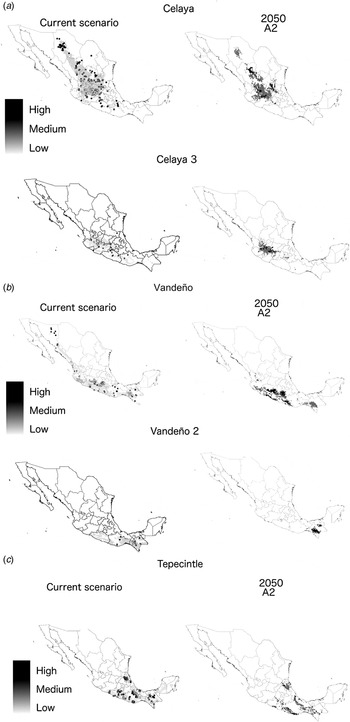
For Vandeño, yield data were mainly collected in Morelos, Jalisco and Chiapas. In these three states, potentially high-yield areas (3000–6000 kg/ha) were found (see Fig. S1 in the Supplementary Material available from http://journals.cambridge.org/AGS). Although most observations come from these three states, there are other records without yield information located in Sonora. The projected high-yield areas under current conditions are in Sonora but also in Oaxaca and Chiapas. Under future climatic conditions, the potential distribution area is reduced by 70% and high yields will be found in the western states of Michoacán and Guerrero. The sub-group Vandeño 2, whose distribution is in the southern part of the country, is projected to potentially have higher yields in both states where observations have taken place: Oaxaca and Chiapas. Under future climatic conditions, distribution decreases by 85% and higher yields can only be found in Chiapas (Fig. 1 b).
Finally, for Tepecintle, observations registered high yields in the three states where yield values were obtained: Veracruz, Chiapas and Oaxaca (1601–4000 kg/ha) (Fig. S1 in the Supplementary Material available from http://journals.cambridge.org/AGS). Under current conditions the model projected potential high-yield areas in the same three states and in Guerrero, where field observations with yield values do not exist. Under climate change conditions, potentially high-yield areas are found in Veracruz, Chiapas, Oaxaca and Guerrero. The distribution of potentially high-yield areas is very similar to that presented under current conditions, but it is still possible to see a small shift closer to the coast (Fig. 1 c). In terms of potential distribution area there is a reduction of c. 75% (Fig. 1 c).
DISCUSSION
Relationship between yield and distance to ecological centroids and optima
Ecological theory has proposed that optimal environmental conditions for a species should be close to its ecological NC, and thus abundance should follow a ‘centre-abundant’ pattern in ecological space (Maguire Reference Maguire1973). Studies have empirically demonstrated that this relationship does exist with abundance and other characteristics, such as genetic diversity (Yañez-Arenas et al. Reference Yañez-Arenas, Martínez-Meyer, Mandujano and Rojas-Soto2012, Reference Yañez-Arenas, Peterson, Mokondoko, Rojas-Soto and Martínez-Meyer2014; Martínez-Meyer et al. Reference Martínez-Meyer, Díaz-Porras, Peterson and Yañez-Arenas2013; Lira-Noriega & Manthey Reference Lira-Noriega and Manthey2014). In the present study, it is possible to observe an inverse relationship between yield and the distance to NC/NO for most races evaluated and consequently it might be a useful approach to predict areas with potential current or future high yields, in cases that such data has not been gathered. The latter is the case for many races and sites of distribution in Mexico.
The current results showed that six races presented a model where distance explained more deviance than the null model. Most of these six races had a greater R 2 value when using distance to the NC than distance to the NO. In contrast, distance to the NO better explained yield changes for Celaya and Tepecintle. Additional factors, besides the bioclimatic variables, might be playing a more important role in the distribution of these two races and consequently the model does not embrace the entire bioclimatic range and fails to find a more realistic environmental centroid. Still, areas with the potential of having greater yields were identified by calculating the distance to NC.
On the other hand, it is intriguing why races such as Cónico Norteño had significant positive correlations between yield and the distance to NC/NO. This result has already been found with wild species (Lira-Noriega & Manthey Reference Lira-Noriega and Manthey2014; Yañez-Arenas et al. Reference Yañez-Arenas, Peterson, Mokondoko, Rojas-Soto and Martínez-Meyer2014), but in this particular case it might be related to the condition of a domesticated species, in which factors such as farming technology or farmers’ preferences in growing a specific race, rather than environmental factors significantly affect yield (Bellon & Brush Reference Bellon and Brush1993; Brush & Perales Reference Brush and Perales2007; Ureta et al. Reference Ureta, González-Salazar, González, Álvarez-Buylla and Martínez-Meyer2013). Cónico Norteño is a race with a wide distribution range and probably has more than one NC or NO; consequently when it is divided into clusters, more meaningful results are recovered (see Supplementary Material Table S2, available from http://journals.cambridge.org/AGS). This race embraces an important amount of varieties adapted to different conditions and some of them probably have strong specific local adaptations, making it very difficult to assign a single optimum condition for the entire race.
Similarly, in other widely distributed races (Olotillo, Ratón and Tuxpeño), there might be more than one NC or NO, and consequently identifying sub-groups of populations that shared ecological/genetic conditions and traits, respectively, helped to better project areas with higher yields. Hence, yields of some such widely distributed races (i.e. Tuxpeño, Vandeño and Cónico Norteño) were better explained by geographic clusters rather than by environmental ones.
In maize, geographic distance has been related to genetic distance (Vigouroux et al. Reference Vigouroux, Glaubitz, Matsuoka, Goodman, Sánchez Gonzáles and Doebley2008) and consequently, populations within the same clusters are expected to have a similar genetic composition and might be similarly impacted by environmental conditions (Mercer & Perales Reference Mercer and Perales2010). Regardless of geographic distance, human and natural selection facilitates local adaptation to specific environmental conditions (Mercer et al. Reference Mercer, Martínez-Vásquez and Perales2008; Mercer & Perales Reference Mercer and Perales2010) and consequently, although groups of populations might not be geographically close, their distant localities may be environmentally similar. Both types of clustering provided information on the intra-racial ecological variability that has already been reported (Doebley et al. Reference Doebley, Goodman and Stuber1985; Mercer & Perales Reference Mercer and Perales2010; Ruiz Corral et al. Reference Ruiz Corral, Sánchez González, Hernández Casillas, Willcox, Ramírez Ojeda, Ramírez Díaz and González Eguiarte2013). In the present study, both clustering types increased the deviance explained for some races, so it cannot be generalized that one was better than the other. But geographic clusters generated a higher number of sub-groups, which is generally not convenient because it reduces within sub-group sample size, an essential element if we are to draw robust statistical inferences. However, in the current work splitting races into bioclimatic clusters produced more accurate models. Therefore, when looking for higher yields in other cultivated species (or abundances in wild species) with large distributions, exploring the cluster approach is recommended. Positive correlations were also found in these sub-groups; still, the majority of races and sub-groups presented a negative correlation between yield and NC/NO. In general, the distance to the NC/NO approach is promising in the field of agro-ecology.
The data generated in the present study could be the basis for recommendations to peasant communities in terms of trying to plant some landraces or varieties (clusters) in areas that are predicted to maximize yield, based on their similarities to those of optimum yield predicted here for each race and/or cluster. It would be interesting to validate the models used here, by empirically testing yield in such predicted areas of high or low yield in areas that are not planted with a particular race or variety now. Once the models and predictions are tested, the tool could be iteratively improved for providing more precise recommendations. Additional efforts to recover more complete yield data in areas where the maize races and varieties are being planted by peasants today should also be made. These data will also be a valuable means to improve the tool proposed in the current work and better predict the areas of high maize yield using native varieties and races.
On the other hand, variables correlated with yield variation as a function of NC/NO distance may be used in landrace breeding programmes such as those implemented by some Mexican native maize races (Smith et al. Reference Smith, Castillo and Gómez2001; Aragón-Cuevas et al. Reference Aragón-Cuevas, Taba, Castro-García, Henrnández-Casillas, Cabrera-Toledo, Alcalá, Ramírez and Taba2003). Such an approach could assist in predicting which traits could be used, as correlated markers, to increase yield under contrasting environmental conditions along a landrace geographic distribution.
Potential distribution and yield under current and future climatic conditions
From the nine races evaluated, three were used because they had a significant negative correlation with the NC/NO and high R 2 values, namely Celaya, Vandeño and Tepecintle, to create maps identifying areas with higher yields under current and future climatic conditions. The future potential distribution area of the three races decreased significantly (~58–84%). Higher yields for Celaya under the future climatic scenario were concentrated in its central area of distribution. High-yield areas in the north and south of its distribution at the race and the sub-group level can be expected to disappear based on the current paper's projections. For Vandeño, at the race level the potentially high-yield areas that are present in the northern state of Sonora were projected to disappear and become concentrated in the central and southern distribution areas. For the Vandeño 2 sub-group, potentially higher yields were only projected for Chiapas. For Tepecintle, potentially high-yield areas in the future are expected to remain in the same states where they have been projected under current conditions. There is a slight shift to areas closer to the coast.
Celaya has been classified as a native race adapted to water stress in at least one part of its life-cycle (Ruiz Corral et al. Reference Ruiz Corral, Sánchez González, Hernández Casillas, Willcox, Ramírez Ojeda, Ramírez Díaz and González Eguiarte2013); consequently it might be able to resist harsh environmental conditions such as those expected in the northern states of Mexico in future. Even if higher yields are not projected in Chihuahua for this race in the future, medium yields are. Under such climatic conditions (as the ones projected for 2050 A2), races such as Celaya would maintain medium and high yields in certain parts of their distribution ranges, or may be used for maize production in other colder areas, which could become warmer in the future.
On the other hand, Vandeño has been identified to be adapted to temporal humid and very humid environments; and Tepecintle to very humid ones (Ruiz Corral et al. Reference Ruiz Corral, Sánchez González, Hernández Casillas, Willcox, Ramírez Ojeda, Ramírez Díaz and González Eguiarte2013). Consequently, higher impacts of climate change are expected for these races. Indeed, clear reductions in their projected distribution areas under the climate change scenarios that were modelled were observed.
Native races are expected to have greater success under harsher environmental conditions than improved varieties (Smith et al. Reference Smith, Castillo and Gómez2001), but it is important to know how well each race may perform in different areas of the country. Agro-biodiversity plays a major role in agriculture under changing environmental conditions, and will continue to do so, because it is required for ‘evolutionary resilience’ (Bellon & van Etten Reference Bellon, van Etten, Jackson, Ford-Lloyd and Parry2014). Nevertheless, the contraction of high-yield areas under climate change conditions might have an important influence on farmers’ choices of what to grow where, and also how to manage their seed stocks. The projections made in the present paper can be used to advise peasants to keep different seed stocks for each local variety and make sure to keep sufficient seed for those varieties that are more resistant to water or high-temperature stress. On the other hand, peasants who rely on races adapted to milder and more humid conditions might be advised to test breeding with varieties that are more resistant to harsh conditions. Directed seed-exchange programmes among peasants managing seed for races adapted to different environmental conditions should be planned. In general, seed exchange may on its own favour adaptability under climate change scenarios. Hence, besides the locally adapted varieties, programmes to generate varieties with more genetic variation that enable them to grow under more marginal conditions should be also developed. In any case, programmes that identify genotypes and phenotypes that enable high yield under harsher conditions, in terms of water and temperature stress, for each race or variety/cluster, should be implemented in cooperation with local communities. In each case, local seed-banks for possible harsher conditions should be promoted and tested. The type of modelling proposed in the present study is a first step towards this aim. As stated above, this type of platform should be extended to additional races, more complete yield data gathered and incorporated, and should be improved with empirical data.
SUPPLEMENTARY MATERIAL
The supplementary material for this paper can be found at http://journals.cambridge.org/AGS
We would like to thank el Posgrado en Ciencias Biológicas and CONACyT for the Ph.D. scholarships given to two of the authors and to support the following projects: 240180, 180380, 167705, 152649. We would also like to thank the Dirección General de Análisis y Prioridades of CONABIO for providing the maize database. Finally, we would also like to thank UNAM-DGAPA-PAPIIT: IN203113, IN 203214, IN203814.


