


1. Introduction
Multigenerational co-residence is traditionally highly valued in China (Guo et al., Reference Guo, Li, Yi and Zhang2018; Xu, Reference Xu2019). Due to a poorly developed social welfare system, parents are heavily dependent on their children – both physically and economically – in their old age (Zhao & Zhong, Reference Zhao and Zhong2019). In exchange for eldercare, they invest as much as they can in their children's education and marriage. It is also common for parents to support their co-resident married children and children-in-law by providing free accommodation, food, and childcare (Zhang et al., Reference Zhang, Gu and Luo2014).
Yet, due to globalization, urbanization, and the diffusion of Western values, more and more young people move out of their parents' homes (Xu et al., Reference Xu, Wang and Qi2019). This tendency was accentuated after 2008, when, to alleviate the effects of the Global Financial Crisis, China implemented a massive economic stimulus package (the “Four Trillion” Economic Stimulus Plan) and, as a result, maintained a relatively high economic growth rate compared to many other countries (Burdekin & Weidenmier, Reference Burdekin and Weidenmier2015; Liu et al., Reference Liu, Pan and Tian2018). This growth was accompanied by an accelerated pace of urbanization and industrialization, which led to a significant rural-to-urban migration trend, as urban areas promised higher incomes and better living conditions. At the same time, a growing number of older adults prefer to live nearby their children instead of cohabiting with them, primarily to preserve their autonomy and freedom (Meng et al., Reference Meng, Xu, He, Zhang and Lin2017). In line with these arguments, Giles et al. (Reference Giles, Wang and Zhao2010) document that while around 70% of Chinese adults aged over 60 and living in rural areas co-habited with an adult child in 1991, this percentage had fallen to 40% by 2006.Footnote 1 This trend has been continuing in recent years: data from the China Health and Retirement Longitudinal Study (CHARLS) suggest that 19.79% of families experienced the departure of a member of the younger generation between 2011 and 2013.Footnote 2
This paper investigates how the resources freed up when a member of the younger generation moves out of a household are reallocated. Do the remaining household members consume the resources freed up by the young leaver? Do they save them? Or do they transfer them to the offspring who recently moved out?
Although a number of theoretical and empirical studies emphasize the role of demographics on household consumption and saving patterns (Curtis et al., Reference Curtis, Lugauer and Mark2015; Deaton et al., Reference Deaton, Ruiz-Castillo and Thomas1989; Ge et al., Reference Ge, Tao Yang and Zhang2018; Modigliani & Brumberg, Reference Modigliani, Brumberg and Kurihara1955), only a few studies focus on the effects of changes in household composition on consumption, looking at how resources are reallocated in a household with a child moving out. Among these, Coe and Webb (Reference Coe and Webb2010) and Dushi et al. (Reference Dushi, Munnell, Sanzenbacher, Webb and Chen2021) argue that US parents use most of the resources freed up after the departure of a child to increase their consumption. Focusing on German and Italian households, Rottke and Klos (Reference Rottke and Klos2016) show that part of the freed-up resources is saved and part is consumed.Footnote 3
We extend this body of work in three ways. First, for the first time, we focus on the Chinese case, which is important in light of the trends documented above. Second, considering that multigenerational co-residence is traditionally highly valued in China (Guo et al., Reference Guo, Li, Yi and Zhang2018; Xu, Reference Xu2019) and that around 40% of children are taken care of by their grandparents (Deng & Tong, Reference Deng and Tong2020), we consider, for the first time, the departure of grandchildren and children-in-law, in addition to the departure of children. Third, we take into account the effects of the age of the leavers, which has been overlooked in previous literature. This is important as the resources freed up by the leavers are likely to vary depending on their age (Fernández-Villaverde & Krueger, Reference Fernández-Villaverde and Krueger2007). Moreover, people of different ages are likely to move out of their households for different reasons. This will, in turn, impact how remaining household members deal with the resources freed up by their departure.
Using data from the 2011 and 2013 waves of the CHARLS, we find that, after the departure of a member of the younger generation, on average, the remaining household members save part of the resources freed up by the leaver and consume another part. Although broadly consistent with Rottke and Klos's (Reference Rottke and Klos2016) findings, this result is in sharp contrast with Coe and Webb (Reference Coe and Webb2010) and Dushi et al. (Reference Dushi, Munnell, Sanzenbacher, Webb and Chen2021) who document that the remaining household members generally consume the resources freed up by the leaver. It confirms the strong saving motivations characterizing Chinese households, which could be a consequence of the low social welfare benefits and poor development characterizing the Chinese financial markets (Chamon & Prasad, Reference Chamon and Prasad2010; Cheng et al., Reference Cheng, Liu, Zhang and Zhao2018b).
Differentiating the leavers by age, we find that if the leavers are aged 0–24, the remaining household members save the resources freed up by their departure. By contrast, if the leavers are above 24, then the remaining household members spend the freed-up resources.Footnote 4 Our results are robust to the use of different specifications, different estimation methods including propensity score matching (PSM), as well as different consumption aggregates. Finally, we show that households with young leavers do not increase outward remittances to their non-resident offspring, confirming that they save or consume the freed-up resources rather than providing financial support to the offspring who recently moved out.
The remainder of the paper proceeds as follows. Section 2 surveys some related literature and highlights our contribution. Section 3 illustrates our dataset and presents some descriptive statistics. Section 4 describes our baseline specifications and estimation methodology. Section 5 presents our main empirical results. Section 6 describes a number of further tests. Section 7 discusses whether households with young leavers increase outward remittances to their non-resident offspring. Section 8 concludes.
2. Related literature
Although a number of theoretical and empirical studies emphasize the role of demographics on household consumption and saving patterns (e.g., Curtis et al., Reference Curtis, Lugauer and Mark2015; Deaton et al., Reference Deaton, Ruiz-Castillo and Thomas1989; Ge et al., Reference Ge, Tao Yang and Zhang2018; Modigliani & Brumberg, Reference Modigliani, Brumberg and Kurihara1955), only a few studies focus on the effects of changes in household composition on consumption/saving, looking at how resources are reallocated in a household with a child moving out. These can be divided into two groups. The first focuses on the effects of changes in household composition due to the departure of children for any reason, whilst the second focuses on the effects of changes in household composition due to migration.
2.1 Studies focused on the departure of children for any reason
A few studies, mainly focused on developed countries, look at how resources are reallocated in a household with a child moving out. Among these, making use of data from Italy and Germany, Rottke and Klos (Reference Rottke and Klos2016) find that overall household consumption drops after a child moves out of the household, but at the same time, adult-equivalent consumption significantly increases. In other words, after a child's departure, parents upgrade their personal lifestyle, but also save a fraction of the resources freed up by the departing child.
Focusing on the US, Coe and Webb (Reference Coe and Webb2010) find no evidence that households decrease consumption after children leave, coupled with a significant rise in consumption per capita. This suggests that the resources freed up by the departed children are entirely consumed. Dushi et al. (Reference Dushi, Munnell, Sanzenbacher, Webb and Chen2021) also focus on US data and find that households in their sample only slightly increase 401(k) contributions after children move out. They conclude, once again, that the majority of the resources freed up by the departing child are consumed. Finally, Biggs et al. (Reference Biggs, Chen and Munnell2021) document that after the departure of their offspring, US parents do not save by paying off their mortgage or other debt, do not transfer resources to their departed children, but reduce their hours worked.
2.2 Studies focused on migration
The papers discussed in the previous sub-section do not specify the reason why the children move out of their households. Children may leave for a number of reasons such as going to college, becoming financially independent, getting married and so on. Another reason for departing may be migration. A large literature has looked at the effects of migration on the labor supply, education, and health of the left-behind household members such as parents, spouses, and/or children (see Antman, Reference Antman2012, for a review of this literature). A few studies, mainly focused on developing countries, investigate how the migration of household members affects the food consumption and/or food security of left-behind families. For instance, Abebaw et al. (Reference Abebaw, Admassie, Kassa and Padoch2020) find that Ethiopian households with migrants increase the number of daily calories they consume. Nguyen and Winters (Reference Nguyen and Winters2011) reach a similar conclusion for Vietnam. These findings can be explained by the migrants' higher income, part of which is sent home in the form of remittances. Focusing on China, Liu et al. (Reference Liu, Eriksson and Yi2021) document that the migration of offspring is associated with a significant improvement of the nutritional status of their left-behind parents. By contrast, Karamba et al. (Reference Karamba, Quiñones and Winters2011) argue that households in Ghana generally do not significantly increase their food consumption when a household member migrates, as remittances to the left-behind families are not sufficient to compensate for the loss of labor.
Only a few studies investigate the impact of migration on the overall consumption of the left-behind household members. Among these Chandrasekhar et al. (Reference Chandrasekhar, Das and Sharma2015) find that households with short-term migrants show a lower consumption per capita in India. These migrants generally work in the unorganized sector without formal contracts or legislation to protect their rights. As a result, their salary is relatively low, and they are not able to transfer a significant amount of money back to their left-behind family members. Romano and Traverso (Reference Romano and Traverso2019) argue that international migration only positively affects the per capita consumption of the poorest left-behind households in Bangladesh. In the context of China, Wang et al. (Reference Wang, Liu and Yan2021) make use of the 2013 wave of the CHARLS and find that elderly households with permanent migrant children show a higher share of expenditure on agriculture, whilst households with temporary migrant children show a higher share of food consumption.Footnote 5 It is, however, noteworthy that these studies make use of cross-sectional data. As such, they compare the consumption patterns of households with migrants and households without. Their focus is, therefore, different from the papers surveyed in the previous sub-section which look at the effect of the actual moving out of children between one wave and the other on the consumption of left-behind household members in a panel setting.
2.3 Contribution
Our paper speaks to these two branches of literature by analyzing the effects of the departure of members of the younger generation on the consumption of the left-behind household members in China.
Specifically, our work adds to the literature surveyed in Section 2.1 in three ways. First, for the first time, we focus on the effects of the departure of members of the younger generation on consumption in the Chinese context. This is important bearing in mind that, as a result of globalization, urbanization, and the diffusion of Western values, more and more Chinese young people move out of their parents' homes (Xu et al., Reference Xu, Wang and Qi2019). Second, considering that multigenerational co-residence is traditionally highly valued in China (Guo et al., Reference Guo, Li, Yi and Zhang2018; Xu, Reference Xu2019) and that around 40% of children are taken care of by their grandparents (Deng & Tong, Reference Deng and Tong2020), we consider, for the first time, the departure of grandchildren and children-in-law, in addition to the departure of children. Third, we take into account the effects of the age of the leavers, which has been overlooked in previous literature. This is important as the resources freed up by the leavers are likely to vary depending on their age (Fernández-Villaverde & Krueger, Reference Fernández-Villaverde and Krueger2007). Moreover, people of different ages are likely to move out of their households for different reasons. This will, in turn, impact how remaining household members deal with the resources freed up by their departure.
In our setting, one of the possible reasons why children leave their household is migration. Thus, our work also relates to the small literature which has looked at the effects of migration on total household consumption by making use of a panel data setting. This enables us to look at the effects of offspring actually moving out of the household between one wave and another.
3. Data and summary statistics
3.1 Sample construction
Our analysis is based on the 2011 and 2013 waves of the CHARLS. The survey, which is nationally representative, collects high-quality data for residents aged 45 and above and their spouses.Footnote 6 10,026 households took part in the 2011 wave and 10,624 households in the 2013 wave.Footnote 7 Information is also provided about how many additional household members there are, their relationship to the main respondent, and their age.
In order to compare consumption changes between 2011 and 2013 in households with and without leavers, we only consider the 8,786 households who participated in both waves. As the age structure of the household members is a key factor in our analysis, we exclude 1,726 households with missing age information on some of the members. We also exclude 376 households that reported additional members in 2013.Footnote 8 Furthermore, as the CHARLS focuses on respondents aged 45 and above, we drop households whose main respondent and/or spouse is aged under 45. This leaves us with 6,843 households. Next, in order to deal with outliers, we set to missing the top and bottom 1% observations of total, non-durables, and non-education expenditure, household income, and household financial wealth. Finally, we exclude observations with missing values for variables included in our models. This leaves us with 11,640 observations over the two years, corresponding to 6,584 households.
3.2 Summary statistics
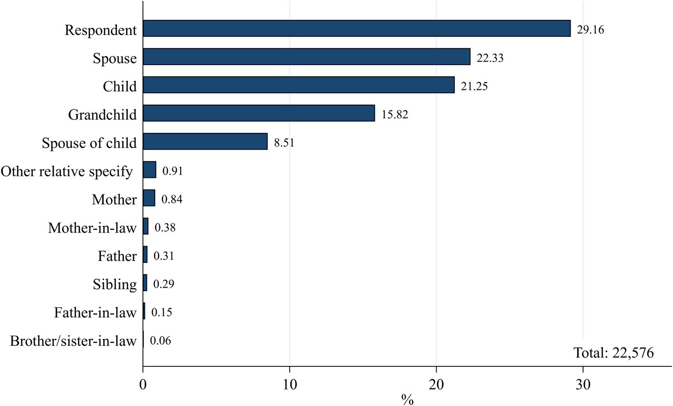
Our sample is composed of 6,584 households with a total of 22,567 members. Figure 1 shows that more than 51% of these household members are main respondents (29.16%) and their spouses (22.33%). Children and grandchildren account for 21.25 and 15.82% of the total household members, respectively. If we also consider children-in-law, the younger generations' members account for 45.58% of the total.
Household composition (percentage) in the CHARLS (2011).
Note: The data is based on our main regression sample where respondents were aged 45 and above in both waves of the survey, and households participated in both waves of the survey and provided age information for every household member.
Source: Authors' calculations based on the CHARLS.

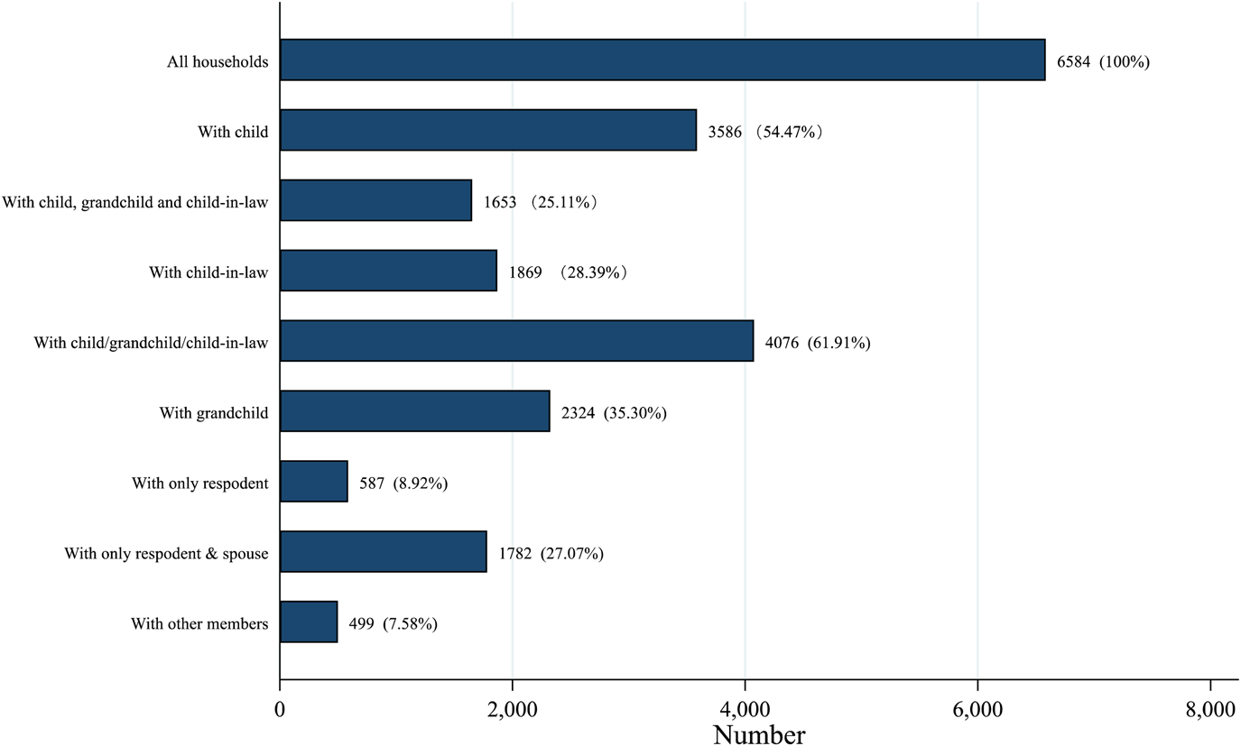
Figure 2 shows that 4,076 out of 6,584 households (61.91%) in our dataset have members of at least two generations within the family home (i.e., parents living with children/children-in-law and/or grandchildren). There are 1,653 households (25.11%) with at least three generations residing within the family home (i.e., parents, children/children-in-law, and grandchildren), and 1,782 households (27.07%) which only consist of respondent and spouse. These statistics illustrate the diverse composition of Chinese households.
Number (percentage) of households by composition in the CHARLS (2011).
Note: “All Households” are the households used in our main regression models. “With only respondent” represents the households with only one member. “With only respondent and spouse” are the households composed of only the main respondent and his/her spouse. “With child” represents the households with at least one child in residence. “With grandchild” stands for the households with at least one grandchild in residence. “With child-in-law” stands for the households with at least one child-in-law in residence. “With child/grandchild/child-in-law” stands for the households with at least one member of the younger generation in residence. “With child, grandchild, and child-in-law” represents the households who have at least three generations in residence. “With other members” stands for the households with at least one other household member (different from spouse, child, grandchild, and child-in-law) in residence. There are overlaps between certain groups.
Source: Authors' calculations based on the CHARLS.

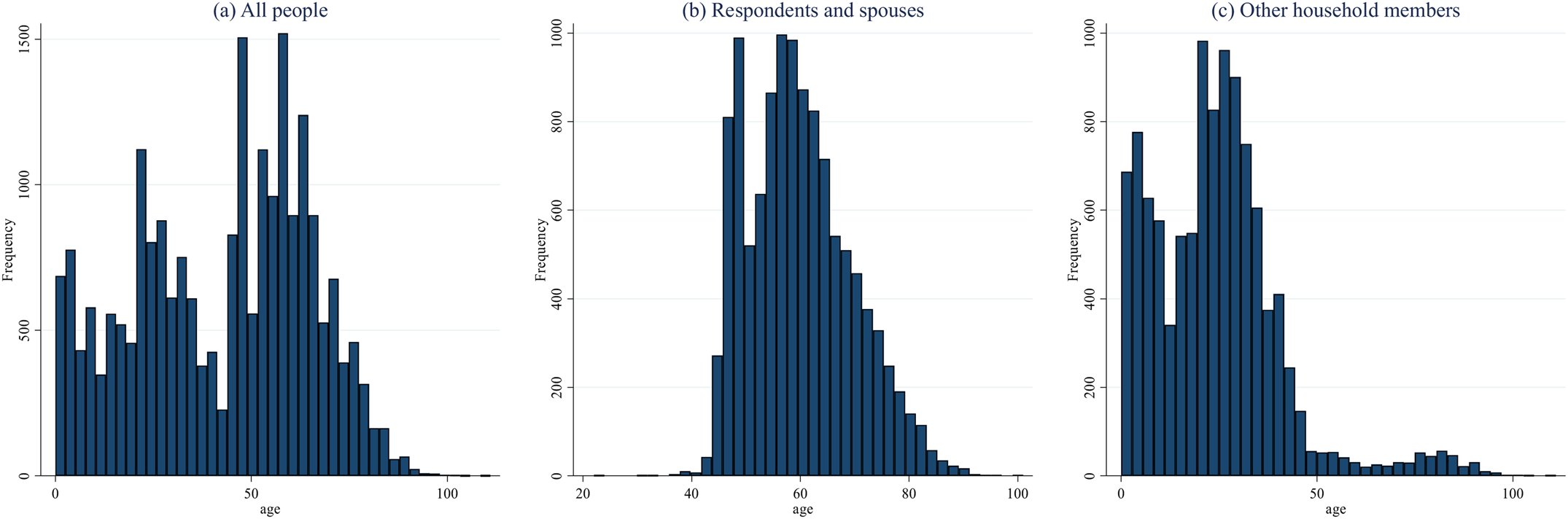
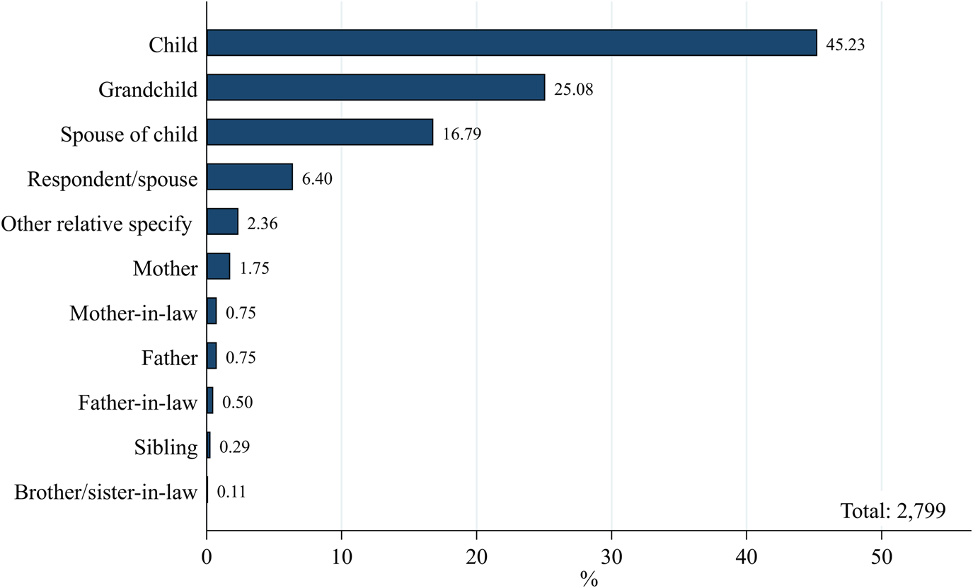
Figure 3 shows the age distribution of household members. 96.24% of main respondents and spouses are aged between 45 and 80. Among other household members, 94.74% are aged between 0 and 50, with more than 93% belonging to the younger generation (children, children-in-law, and grandchildren of main respondents). Leavers are defined as those who were family members in 2011 but not in 2013 due to moving out from the family home, death, or other reasons. In our sample, 2,799 leavers are reported from within 1,534 households. Figure 4 shows that 87.1% of these leavers belong to younger generations: they are main respondents' children (45.23%), grandchildren (25.08%) and children-in-law (16.79%).
Age distribution in the CHARLS (2011).
Note: The data is based on our main regression sample where respondents were aged 45 and above in both waves of the survey, and households participated in both waves of the survey and provided age information for every household member. “Other household members” represents all the household members apart from respondents and their spouses.
Source: Authors' calculations based on the CHARLS.

Leavers (percentage) in the CHARLS (2013).
Note: The data is based on our main regression sample where respondents were aged 45 and above in both waves of the survey, and households participated in both waves of the survey and provided age information for every household member.
Source: Authors' calculations based on the CHARLS.

Figure 5 presents the ages of leavers in different categories: The leavers' age ranges from 0 to 111.Footnote 9 The most common age range of child leavers is between 20 and 40, which accounts for 88.63% of the total child leavers, and the mean age of a child leaver is 28. Children typically move out of the household when they start their own family and/or become financially independent, which usually happens when they are in their late twenties. Figure 5 also shows that grandchild leavers aged between 0 and 20 count for 92.74% of the total leavers in this category, with a mean age of 10. Most younger generation's household members who move out at ages between 0 and 16 are grandchildren of main respondents. In China, it is normal for grandparents to live with and look after their grandchildren at least for some time (Deng & Tong, Reference Deng and Tong2020; He et al., Reference He, Li and Wang2018b). Finally, 96.6% of leaving children-in-law are aged between 20 and 45, and the mean age of leavers in this category is 32.
Age distribution of leavers in the CHARLS (2013).
Note: The data is based on our main regression sample where respondents were aged 45 and above in both waves of the survey, and households participated in both waves of the survey and provided age information for every household member.
Source: Authors' calculations based on the CHARLS.

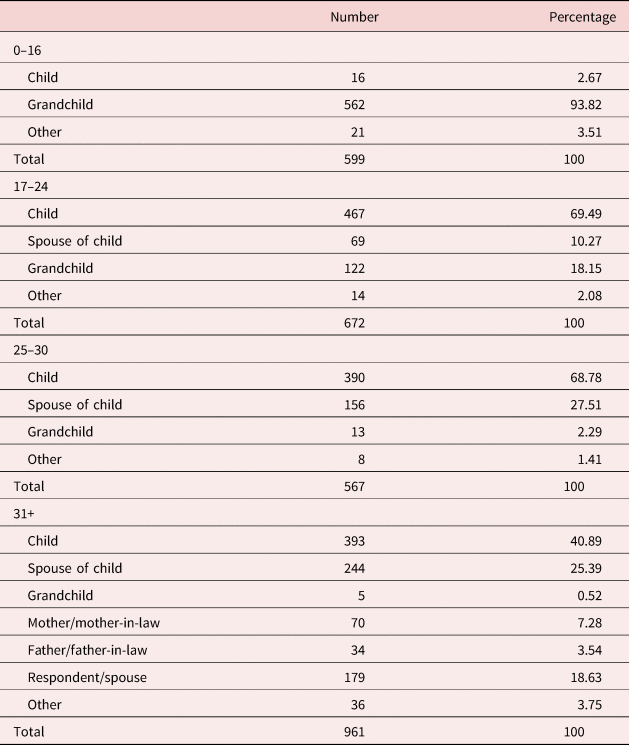
Table 1 presents the composition of leavers across different age groups. We can see that just under 94% of leavers in the age range 0–16 are grandchildren of the respondent. This percentage drops to 18.15% in the age range 17–24, and to 2.29% in the range 25–30. The percentage of children/spouses of children leaving the household ranges from 2.67% in the range 0–16, to 79.76% in the range 17–24, and to 96.29% in the 25–30 range. In the 31+ range, only less than 1% of leavers are grandchildren, 66.28% are children/spouse of children, and the remaining leavers are other household members (e.g., mother, father, and so on).
Leavers by age group

Note: The data is based on our main regression sample where respondents were aged 45 and above in both waves of the survey, and households participated in both waves of the survey and provided age information for every household member.
Source: Authors' calculations based on the CHARLS.
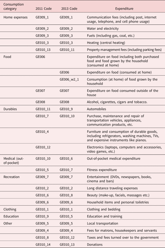
Table 2 presents details of the various consumption categories that we consider. Appendix Table A1 presents definitions of all other variables used in the paper. Appendix Tables A2, A3, and A4 respectively present descriptive statistics for different categories of consumption, consumption changes of household with leavers between 2011 and 2013, and all the variables used in our models. It is noteworthy that according to Appendix Table A3, the average age of the main respondents in our sample is 61.34. Moreover, the average household size is 3.4 and 37.47% of households are from urban areas. Finally, 89.02% of respondents own their house.
Consumption categories

Note: All consumption categories provided by the CHARLS are listed in the table. We further categorize them following Meyer (Reference Meyer2013).
Source: 2011 and 2013 waves of the CHARLS.
4. Baseline models
4.1 Models accounting for the departure of members of the household's younger generation
We start by studying the response of total, non-durable, and non-education consumption to the departure of any member of the household's younger generation. To this end, we estimate the following equation:

where log C j,t represents in turn the logarithm of the real total, non-durable, and non-education consumption for household j in year t. We estimate the models for the above-mentioned consumption aggregates in levels and per capita.Footnote 10 Following Coe and Webb (Reference Coe and Webb2010) and Rottke and Klos (Reference Rottke and Klos2016), we focus on both total and non-durable consumption because the latter is likely to be the most responsive to changes in household composition.Footnote 11 We add non-education expenditure to investigate the extent to which changes in total/non-durable consumption are driven by changes in education expenditure, once a member of the household's younger generation leaves the household. YoungMove j,t indicates the number of members of the younger generation who moved out of household j between 2011 and 2013.Footnote 12, Footnote 13
Controlsj,t represents a set of control variables. Specifically, following Rottke and Klos (Reference Rottke and Klos2016), we control for the main respondent's age, marital and health status, as well as for total household financial wealth and home ownership.Footnote 14 We also include the number of non-offspring household members,Footnote 15 as well as household income, which is defined as the sum of the income of all household members. This comprises salaries, pensions, benefits, and asset revenues of all household members, as well as remittances from non-resident children and grandchildren.Footnote 16
Following Danziger et al. (Reference Danziger, Van Der Gaag, Smolensky and Taussig1982) and Robb and Burbidge (Reference Robb and Burbidge1989) who document that consumption demand decreases with age in the late stages of the life cycle, we expect the sign of the coefficient associated with the main respondent's age to be negative. Compared with singles, married people face less uncertainty in their income and consumption as their partners will support them when they encounter financial problems. Thus, marriage can be regarded as a form of insurance against income and health risks (Yang & De Nardi, Reference Yang and De Nardi2016). We therefore expect a positive association between the dummy variable indicating that the respondent is married and household consumption. Furthermore, considering the low level of social welfare benefits in China (Cheng et al., Reference Cheng, Liu, Zhang and Zhao2018b), we expect people with poorer health to incur higher out-of-pocket medical expenditures and hence to exhibit higher consumption. In line with Gan et al. (Reference Gan, Yin and Zang2010), we expect homeownership to be associated with a higher consumption. Finally, according to the wealth and income effect, people tend to spend more as their income and/or the value of their assets increase. We therefore anticipate a positive sign on the coefficients associated with total household financial wealth, income, and home ownership (Paiella and Pistaferri, Reference Paiella and Pistaferri2017).
It is particularly important to include income in our equation as the departure of older offspring may affect household consumption indirectly by affecting household income. Specifically, such departures would reduce the leavers' financial contributions to the household, which may, in turn, affect household consumption. Similarly, children who migrate may send remittances back home, which have been found to supplement income in rural China and increase per capita consumption (Démurger & Wang, Reference Démurger and Wang2016). Parents who leave their children behind typically also send remittances back home to help grandparents with the education and upbringing of the children (Secondi, Reference Secondi1997). When they take their children back, they may stop these transfers. All these effects are captured by our household income variable, which includes the salaries of all household members as well as remittances from non-resident household members. As a result, all the effects of the departure of members of the younger generation on the consumption of the remaining household members that we discuss hereafter are net of these changes in income.
The error term in Equation (1) is made up of the following components: u j, which is a household-specific time-invariant effect often referred to as unobserved heterogeneity; u t, which accounts for business cycle effects; the interaction between provincial fixed effects (u p) and time fixed effects (u t), which is aimed at capturing province-specific business cycle effects; and $\varepsilon _{jt}$ , which represents an idiosyncratic error term. To account for the u j component of the error term, we use a fixed-effects estimator.Footnote 17 We report robust standard errors rather than the conventional standard errors to account for potential heteroskedasticity and within-group correlation.
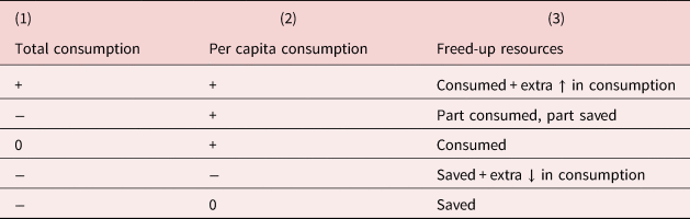
In order to assess how the remaining household members allocate the resources freed up by the leaver, it is necessary to estimate Equation (1) both for household consumption and per capita consumption. Table 3 shows how different coefficients associated with the YoungMove j,t variable in the two equations translate in the freed-up resources being saved and/or consumed.
Conceptual framework

Note: This table reports possible signs of the coefficients associated with number of leavers in the models aimed at explaining total consumption (column 1) and per capita consumption (column 2). Column 3 describes whether according to the combinations of signs in columns 1 and 2, the resources freed up by the leaver are consumed and/or saved.
In a nutshell, if the coefficient associated with YoungMove j,t in the model for per capita consumption is positive, there are three possible scenarios. If the corresponding coefficient in the model for total consumption is also positive, then all the resources freed up by the leaver are consumed and, after the departure, the remaining household members even increase their consumption further compared to the pre-departure period. If the corresponding coefficient in the model for total consumption is not statistically significant, then all freed-up resources are consumed. If it is negative, then part of the freed-up resources is consumed and part is saved.
If the coefficient associated with YoungMove j,t in the model for per capita consumption is negative and the corresponding coefficient in the model for total consumption is also negative, then the freed-up resources are saved and the remaining household members even decrease their overall consumption after the departure compared to the pre-departure period. Finally, if the coefficient associated with YoungMove j,t in the model for per capita consumption is not statistically significant and the corresponding coefficient in the model for total consumption is negative, then all freed-up resources are saved.Footnote 18
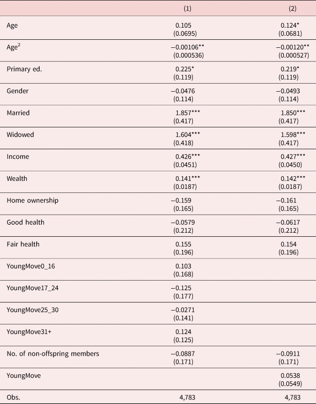
4.2 Differentiating leavers by age
We next examine the extent to which consumption changes according to the age of the leavers. To this end, we estimate the following equation:

YoungMove0_16j,t, YoungMove17_24j,t, YoungMove25_30j,t, and YoungMove31+j,t represent the number of young leavers in each age group in household j in year t.Footnote 19, Footnote 20 The control variables and components of the error term are the same as in Equation (1). Once again, we estimate Equation (2) both for household consumption and per capita consumption, using a fixed-effects estimator. As in the previous sub-section, in order to assess whether the remaining household members save or consume the resources freed up by the leavers, the coefficients associated with the YoungMove variables in the models for per capita consumption need to be interpreted together with those in the models for total consumption.
5. Results
5.1 Do parents/grandparents use the resources freed up following the departure of a member of the younger generation to increase their consumption?
Table 4 shows the estimates of Equation (1). The dependent variables in columns 1–3 are the logarithms of total household consumption, non-durable consumption, and non-education consumption, respectively. The dependent variables in columns 4–6 are the logarithms of total household consumption per capita, non-durable consumption per capita, and non-education consumption per capita respectively, which are calculated by dividing total, non-durable and non-education consumption by household size. Finally, following Rottke and Klos (Reference Rottke and Klos2016), the dependent variables in columns 7–9 are the logarithms of total, non-durable and non-education consumption divided by the equivalence scale (EQS).Footnote 21
Young leavers and household consumption

Note: All models are estimated using a fixed-effects estimator. See Appendix Table A1 for definitions of all variables. The dependent variables in columns 1–3 are the logarithms of total, non-durable, and non-education household consumption, respectively. The dependent variables in columns 4–6 are the logarithms of total, non-durable, and non-education household consumption per capita, respectively, which are calculated by dividing consumption by the number of household members (c/n). The dependent variables in columns 7–9 are the logarithms of adult-equivalent total, non-durable, and non-education household consumption, respectively, which are calculated by dividing consumption by the equivalence scale (n0.8). Year dummies and the interactions between provincial and year dummies are included in all models, but their estimates are not reported for brevity. Robust standard errors are in parentheses. ***, **, and * indicate significance at the 1%, 5%, and 10% levels, respectively.
We can see that whatever the consumption aggregate, household consumption decreases when a household member departs. Specifically, the departure of a member of the younger generation is associated with an 11.91% (column 1), 11.63% (column 2), and 10.41% (column 3) drop in total, non-durable, and non-education consumption, respectively. These findings are consistent with Irvine (Reference Irvine1978) who find that household size has a direct effect on household consumption. They are also consistent with Deaton and Paxson (Reference Deaton and Paxson1998) and Deaton et al. (Reference Deaton, Ruiz-Castillo and Thomas1989) who find that expenditure on food, education, local transportation costs, and personal toiletries increase with the number of household members.
At the same time, the estimates in columns 4–6 (7–9) show a rise in consumption per capita (adult-equivalent consumption) by 16.97, 17.23, and 18.45% (11.19, 11.46, and 12.68%) respectively for total, non-durable, and non-education consumption in association with the departure of an offspring.Footnote 22 In accordance with the conceptual framework in Table 3, this suggests that part of the resources freed up by the leaver are consumed and another part is saved.Footnote 23 Although consistent with Rottke and Klos (Reference Rottke and Klos2016) who also find that part of the resources freed up by the leavers are saved by the remaining household members, these findings are opposite to Coe and Webb (Reference Coe and Webb2010), and Dushi et al. (Reference Dushi, Munnell, Sanzenbacher, Webb and Chen2021), who find that parents generally increase their consumption after children move out. This can be explained considering that Chinese people have stronger incentives to save compared to those in the US (Chamon & Prasad, Reference Chamon and Prasad2010; Cheng et al., Reference Cheng, Liu, Zhang and Zhao2018b).
In terms of the control variables, consistent with Paiella and Pistaferri (Reference Paiella and Pistaferri2017), there is a positive relationship between both household financial wealth and income, and consumption. Similarly, there exists a strong relationship between the marital status of the main respondent and consumption, which is consistent with Yang and De Nardi (Reference Yang and De Nardi2016). Widows also show a higher consumption than their “never married” counterparts probably because they got used to higher living standards whilst married.
5.2 Does the age of the young leavers make a difference?
The literature on how parents allocate newly freed-up resources following a child's departure (Coe & Webb, Reference Coe and Webb2010; Dushi et al., Reference Dushi, Munnell, Sanzenbacher, Webb and Chen2021; Rottke & Klos, Reference Rottke and Klos2016) does not take the leavers' age into account. Given the wide range of leavers' ages shown in our dataset (Fig. 5), we next consider the leavers' age by estimating Equation (2).
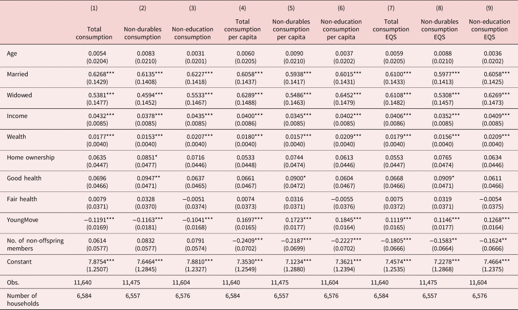
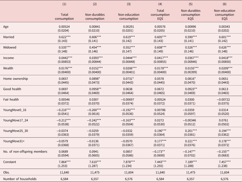
Table 5 presents estimates of Equation (2), obtained using a fixed-effects estimator. The dependent variables in columns 1–3 are the logarithms of total household consumption, non-durable consumption, and non-education consumption, respectively. The dependent variables in columns 4–6 are the logarithms of adult-equivalent total, non-durable and non-education consumption.
Young leavers and household consumption differentiating leavers by age

Note: All models are estimated using a fixed-effects estimator. See Appendix Table A1 for definitions of all variables. The dependent variables in columns 1–3 are the logarithms of total, non-durable, and non-education household consumption, respectively. The dependent variables in columns 4–6 are the logarithms of adult-equivalent total, non-durable, and non-education consumption, respectively, which are calculated by dividing consumption by the equivalence scale (n0.8). Year dummies and the interactions between provincial and year dummies are included in all models, but their estimates are not reported for brevity. Robust standard errors are in parentheses. ***, **, and * indicate significance at the 1%, 5%, and 10% levels, respectively.
Focusing on columns 1–3, we observe that the coefficients associated with offspring leavers aged 0–24 are negative and statistically significant, regardless of the consumption aggregate. Focusing on column 1, households with a leaver aged 0–16 decrease their consumption by 21.6%. The corresponding figure for households with leavers aged 17–24 is 21.2%. Similar figures are observed in columns 2 and 3 for non-durables, and slightly lower figures (respectively 19.2 and 16.3%) are shown for non-education consumption. The corresponding coefficients in the models for adult-equivalent consumption are not statistically significant (columns 4 to 6).
Taken together, these findings suggest that the remaining household members save the resources freed up by leavers aged 0 to 24 and can be explained as follows. Table 1 shows that 93.82% of offspring who move out between the ages of 0 and 16 are grandchildren of main respondents. Grandparents living with grandchildren typically invested significant amounts in the education and upbringing of their children in the past, and they also spend significant amounts for their resident grandchildren. As a result, these grandparents have a strong motivation to save the freed-up resources when their grandchildren move out, in order to smooth their consumption. As for leavers aged between 17 and 24, Table 1 indicates that 69.49% of them are children of the respondents and 18.15% of them are grandchildren. Most of these leavers will have just completed their education. In fact, Chinese people generally complete their education at an age ranging from 18 (when most graduate from high school) to 24 (a common age for completing Masters degrees). When offspring complete their education and move out of the family home, the household consumption on education will drop sharply. Once again, having spent large amounts on the education of their children/grandchildren, parents/grandparents will be inclined to save the resources freed up by the leaver.
These findings confirm Chinese households' strong preference for high savings (Chamon & Prasad, Reference Chamon and Prasad2010). Several factors may contribute to this behavior. First, the Chinese culture places a high value on thrift and precautionary saving (He et al., Reference He, Huang, Liu and Zhu2018a), which was especially pertinent in the uncertain global economic climate post-crisis. Second, the transition from a planned to a market economy, coupled with an underdeveloped social safety net and a poorly developed financial system, may have increased the necessity for households to self-insure through saving (Chamon & Prasad, Reference Chamon and Prasad2010; Cheng et al., Reference Cheng, Liu, Zhang and Zhao2018b). Lastly, rapid aging, changes in family structure due to the one-child policy, and rising housing prices are other key factors which can explain Chinese people's tendency to save a large share of their disposable income (Chamon & Prasad, Reference Chamon and Prasad2010; Zhou, Reference Zhou2014).
By contrast, in columns 1–3 of Table 5, we observe that the coefficients associated with leavers aged 25 and over are not statistically significant, while they are positive and highly significant in the adult-equivalent consumption models (columns 4–6). For instance, focusing on column 4, we observe that households with offspring leavers aged between 25 and 30 increase their total adult-equivalent consumption by 19.0% following the departure of members of the younger generation. The corresponding figure for offspring leavers aged above 30 is 17.7%. Similar patterns are observed for non-durable and non-education consumption in columns 5 and 6. Overall, these results suggest that the remaining household members consume the resources freed up by the leaver. This can be explained bearing in mind that children in this age group who move out of the household have more wealth than those still residing with their parents and, as such, can provide a source of risk-sharing for their parents.Footnote 24 In China, financially independent children are in fact responsible for providing financial and physical support to their dependent parents (Chen et al., Reference Chen, Chen and He2019; Zhang, Reference Zhang2019; Zhang & Harper, Reference Zhang and Harper2022). They are especially important when their parents have to pay unexpected large amounts of money, such as medical expenses. Therefore, children can be regarded as a form of insurance. Gourinchas and Parker (Reference Gourinchas and Parker2002) find evidence that income increases with age during the early working life. In the Chinese context, this implies that the older the children, the stronger their financial capability and their subsequent ability to assist their parents financially. In other words, the reimbursement rate of this special type of insurance (children) increases with the age of the children. Thus, parents with older and independent children face less income uncertainty and, in turn, less need to save for precautionary reasons. This can explain why they tend to consume a larger proportion of the resources freed up when an older child leaves the family home.
6. Further tests
6.1 Robustness tests
We conduct a set of robustness tests. First, Appendix Table A5 shows that our baseline results are robust to using a weighted fixed-effects estimator. Second, Appendix Table A6 shows that they hold when using a balanced panel.Footnote 25 Both these exercises enable us to conclude that our main findings are not driven by attrition. Third, Appendix Table A7 shows that our results are robust to dropping members of the younger generation who passed away or left the household for reasons other than moving out.
Fourth, so far we have looked at the determinants of total, non-durable, and non-education consumption. One may wonder whether the results also hold for specific consumption categories. However, as durable and education consumption are respectively characterized by 61.05 and 72.39% zero values, we are not able to estimate their determinants using a fixed-effects linear estimator. A Tobit estimator should be used in this case, but fixed effects cannot be accounted for due to the incidental parameter problem. In Appendix Table A8, we therefore verify whether our results are robust to focusing on two other consumption aggregates, namely out-of-pocket medical expenditure and “other” expenditure, which either have few or no zero values. The former represents an important share (13.44%) of the total consumption of the respondents in our dataset, is essential expenditure, and closely depends on household composition. The latter is a miscellaneous category which includes diverse items such as local transportation; fees for matrons, housekeepers, and servants; taxes and fees turned over to the government; donations and so on. We can see that our main results hold for these two sub-categories of consumption, with one exception: neither total nor adult-equivalent out-of-pocket medical expenditure are affected by movers aged 25–30. This can be explained bearing in mind that respondents in this age group are generally healthy and may only free up a small amount of resources.Footnote 26
6.2 Differentiating households based in rural and urban areas
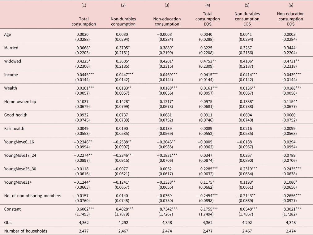
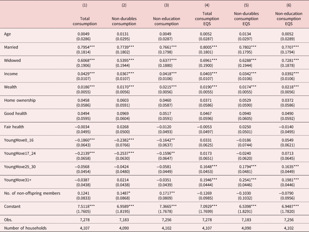
As households living in rural areas may be very different from households based in urban areas, we have conducted separate analyses for households based in the two areas. The results are presented in Tables 6 and 7. In both Tables, the dependent variables in columns 1–3 are the logarithms of total household consumption, non-durable consumption, and non-education consumption, respectively. The dependent variables in columns 4 to 6 are the logarithms of total, non-durable and non-education adult-equivalent consumption.
Young leavers and household consumption differentiating leavers by age; urban sample

Note: All models are estimated using a fixed-effects estimator. See Appendix Table A1 for definitions of all variables. The dependent variables in columns 1–3 are the logarithms of total, non-durable, and non-education household consumption, respectively. The dependent variables in columns 4–6 are the logarithms of adult-equivalent total, non-durable, and non-education consumption, respectively, which are calculated by dividing consumption by the equivalence scale (n0.8). Year dummies and the interactions between provincial and year dummies are included in all models, but their estimates are not reported for brevity. Robust standard errors are in parentheses. ***, **, and * indicate significance at the 1%, 5%, and 10% levels, respectively.
Young leavers and household consumption differentiating leavers by age; rural sample

Note: All models are estimated using a fixed-effects estimator. See Appendix Table A1 for definitions of all variables. The dependent variables in columns 1–3 are the logarithms of total, non-durable, and non-education household consumption, respectively. The dependent variables in columns 4–6 are the logarithms of adult-equivalent total, non-durable, and non-education consumption, respectively, which are calculated by dividing consumption by the equivalence scale (n0.8). Year dummies and the interactions between provincial and year dummies are included in all models, but their estimates are not reported for brevity. Robust standard errors are in parentheses. ***, **, and * indicate significance at the 1%, 5%, and 10% levels, respectively.
For movers aged 0–30, these Tables show broadly similar results in urban and rural areas, which are also very similar to the baseline results. Specifically, we observe negative coefficients associated with the number of leavers aged 0–24 in the models for total, non-durable, and non-education consumption, coupled with insignificant coefficients in the corresponding regressions for adult-equivalent consumption. This suggests that the remaining household members save the resources freed up by the leavers. Focusing on the leavers aged 25–30, we observe positive coefficients associated with the adult-equivalent consumption aggregates and insignificant coefficients associated with the total aggregates. This suggests that the remaining household members consume the resources freed up by these leavers.
The Tables highlight, however, one difference between rural and urban areas. In rural areas, leavers aged 31 or more are associated with a higher adult-equivalent consumption of the left-behind household members (columns 4–6), coupled with an unchanged total consumption (columns 1–3). This suggests that regardless of the consumption aggregate considered, the remaining household members consume the resources freed up by the leaver. Yet, in urban areas, the results show negative (albeit only marginally significant) coefficients associated with these same leavers in columns 1–3, coupled with positive coefficients for the adult-equivalent aggregates (columns 4–6), which indicates that the remaining household members consume only part of the resources freed up by the leaver and save the rest. This difference between rural and urban areas could be explained bearing in mind that parents with leavers aged 31 and above are typically older and realize that they may need more help and support both financially and in-kind going forward. Whilst in rural areas, due to tighter social networks, support can be more easily obtained from friends, neighbors, and relatives living outside the household, this may be more difficult in big cities, which could then trigger a tendency of left-behind household members to save part of the resources freed up by the leaver for precautionary reasons. Another reason why households with leavers aged 31 or above may save part of the resources freed up by the leaver in urban areas, but not in rural areas may be that pension payments are a larger concern for urban households due to persistent increases in living expenses. By contrast, they are less of an issue in rural areas where many residents rely on self-sufficient agriculture (Zhang et al., Reference Zhang, Brooks, Ding, Ding, He, Lu and Mano2018).
6.3 Propensity score matching (PSM)
The key challenge of evaluating the causal link between the departure of offspring and the consumption of the left-behind household members is to make sure any changes in consumption are due to the departure of the offspring and would not have occurred without that departure. However, in real life, it is impossible to observe the outcome in the absence of the event. Hence, although we make use of panel estimators and control for a wide variety of individual- and household-specific characteristics in our models, which help alleviate the endogeneity concerns arising from omitted variable bias, our findings so far do not necessarily reflect causal relationships between leavers and household consumption.Footnote 27
To better understand the links between the departure of members of the younger generation and consumption of the remaining household members, we make use of PSM (Rosenbaum & Rubin, Reference Rosenbaum and Rubin1983). PSM is a technique that mimics randomization in an observational data set by creating two groups (a treatment and a control group) that are comparable on observed characteristics. As a result, bias attributable to confounding is significantly reduced and selection bias is alleviated.
6.3.1 Methodological considerations
We first estimate Probit regressions to assess the probability of having at least one young leaver in a given age range (i.e., the probability of being treated) as a function of all control variables used in the baseline models evaluated in 2011. Fitted values from these regressions give the propensity scores, which are used to identify households in the control group (i.e., households who share the same characteristics as the treated households, but do not have young leavers) and form the basis of our matching.
Second, we use the one-to-one nearest neighbor matching with replacement, which matches each treated household with the control unit which is closest in terms of propensity score (Rosenbaum & Rubin, Reference Rosenbaum and Rubin1983). When matching with replacement, comparison units can be used as matches more than once if necessary.Footnote 28 We use the caliper matching method, in which caliper refers to the difference in the predicted probabilities between the treated and control households. We match within a caliper of 1%.
Third, following Rottke and Klos (Reference Rottke and Klos2016), we define the average treatment effect of the treated (ATT) as follows:

where Y represents changes in adult-equivalent consumption between 2011 and 2013; the subscripts 1 and 0 refer to households with and without leavers in the age group considered, respectively; and D = 1 denotes the presence of leavers in that age group. At the household level, the first term on the right-hand side of Equation (3) represents the change in adult-equivalent consumption of household X, which has young leavers in the given age range. The second term represents the counterfactual: it measures what the change in adult-equivalent consumption of a household with young leavers in a given age bracket would have been had this household not had leavers. As this counterfactual is unobservable for household X, we seek an alternative household, Z (taken from the control group), with the same characteristics as household X, and observe their change in adult-equivalent consumption. In other words, we use this as a surrogate outcome for household X's counterfactual outcome. Extending this to a group level enables us to calculate the ATTs.Footnote 29
In our context, the ATTs are defined as the expected differences in changes in adult-equivalent consumption over the period 2011–2013 between the treated and the control group.Footnote 30 Any observed difference can be attributed to the departure of offspring in the age range considered. In other words, the ATTs represent the effect of experiencing the departure of a member of the younger generation in a given age range on changes in adult-equivalent consumption for households who actually experienced the departure.Footnote 31
6.3.2 Balancing tests
A series of t-tests suggest that, despite the relatively large size of our sample, for almost all our conditioning variables, the null hypothesis of no difference in means between treated and matched controls after matching could not be rejected. This is reassuring as the t-tests are heavily dependent on sample size (Imbens & Wooldridge, Reference Imbens and Wooldridge2009). We can therefore conclude that the quality of our matching is good. These t-tests are not reported for brevity but are available upon request.
6.3.3 Results
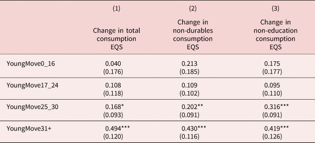
We report the ATTs for households with leavers in various age groups in Table 8. Columns 1–3 respectively refer to changes in adult-equivalent total, non-durable, and non-education consumption. All results are broadly consistent with our previous findings. They suggest that only households with leavers aged 25 and above show statistically significant and positive ATTs. In other words, regardless of how consumption is measured, compared to similar households with no leavers, only households with leavers aged 25–30 and above 30 show a statistically significant premium in adult-equivalent consumption growth, which is likely due to the departure of the offspring(s). In all specifications, the latter households always show the highest ATTs. By contrast, households with leavers younger than 25 show statistically insignificant ATTs.
Average treatment effects on the treated (ATTs)

Note: This table reports the ATTs together with their standard errors. These are obtained using PSM with one-to-one nearest-neighbor matching and caliper of 1%. Columns 1–3 respectively refer to changes in adult-equivalent total, non-durable, and non-education consumption, calculated by dividing total, non-durable, and non-education consumption by the equivalence scale (n0.8). See Appendix Table A1 for definitions of all variables. ***, **, and * indicate significance at the 1%, 5%, and 10% levels, respectively.
7. Do households increase remittances towards non-resident offspring after the departure of a member of the younger generation?
The household consumption analyzed so far does not include households' remittances to non-resident relatives. It is, however, possible that to provide financial assistance to those offspring who departed from home, rather than either save for retirement or consume the freed-up resources, the main respondents opt to transfer these freed-up resources to their offspring leavers, especially in the early stage of their departure (Biggs et al., Reference Biggs, Chen and Munnell2021).
To see whether this is the case, we examine whether household remittances directed towards non-resident children and grandchildren increase after a member moves out from the family home. To this end, we estimate a model of the logarithm of real remittances towards non-resident children and grandchildren as a function of dummies denoting the moving-out of different members of the household's younger generation and control variables.Footnote 32 Specifically, following Xie and Zhu (Reference Xie and Zhu2009), Murphy et al. (Reference Murphy, Kowal, Albertini, Rechel, Chatterji and Hanson2018), and Biggs et al. (Reference Biggs, Chen and Munnell2021), our models control for age, education, gender, health and marital status of the main respondent, as well as for household income and financial wealth. We also include a dummy equal to 1 if the main respondent is a homeowner, and 0 otherwise. Provincial dummies and the number of non-offspring household members are also included in our models. Because remittances are censored at 0, we use a Tobit estimator. The results are reported in Table 9.Footnote 33 In column 1, the leavers are differentiated by age, whilst in column 2, they are not.
Young leavers and remittances directed to non-resident members of the younger generation (2013)

Note: The dependent variable in both columns is the remittances directed towards non-resident members of the younger generation. The equation is estimated using a Tobit estimator, and marginal effects are reported, with standard errors in parentheses. Provincial dummies are included in all models, but their coefficients are not reported for brevity. See Appendix Table A1 for definitions of all variables. ***, **, and * indicate significance at the 1%, 5% and 10% levels, respectively.
Focusing on column 1, we can see that for all age groups of young leavers, the moving out of a member of the younger generation is not significantly associated with changes in remittances directed towards non-resident children and grandchildren. In column 2, we use the total number of members of the younger generation who move out (YoungMove) as the key explanatory variable. As before, the results show that households do not increase their remittances to non-resident offspring after their departure. These findings, which are consistent with Biggs et al. (Reference Biggs, Chen and Munnell2021), suggest that parents/grandparents do not transfer the resources freed up when the children and grandchildren move out to the leavers as a type of further financial support.
Focusing on the coefficients associated with the control variables, columns 1 and 2 of Table 9 show an inverse U-shaped relationship between the age of the main respondent and the amount of outward remittances to the younger generations. In addition, there is a strong positive relationship between education and household outward remittances, which implies that residents who have completed primary education support non-resident relatives to a greater extent when compared to their less educated counterparts. Compared with single people, married people tend to have a larger extended family, leading to a positive relationship between marital status and outward remittances. Finally, our results show that household income and wealth are positively related to outward remittances. In China, due to the poorly developed financial system, relatives and friends are the main sources of funding for households (Zhou, Reference Zhou2014). As a result, households with high wealth typically provide more financial assistance to their non-resident younger relatives.
8. Conclusion
Based on a panel of 6,548 middle-aged and elderly households taken from the CHARLS over the period 2011–2013, we investigate how the remaining household members deal with the resources freed up after the departure of members of the younger generation. We find that, on average, the remaining household members save part of the resources freed up by the leaver and consume another part. Although broadly consistent with Rottke and Klos's (Reference Rottke and Klos2016) findings for Germany and Italy, this result is opposite to Coe and Webb (Reference Coe and Webb2010) and Dushi et al. (Reference Dushi, Munnell, Sanzenbacher, Webb and Chen2021), who document that in the US, parents generally increase their consumption after children move out.
Next, we find that the reallocation of the resources freed up by the leavers closely depends on the leavers' age. Specifically, if the leavers are aged 24 or below, the remaining household members save all the freed-up resources. By contrast, if the offspring leavers are aged above 24, the remaining household members spend the freed-up resources. Our results are robust to the use of different specifications, different consumption aggregates, and different estimation methods including PSM. Finally, we find no evidence that parents/grandparents transfer the resources freed up when the children/grandchildren move out to the leavers as further financial support.
Our study suffers from a number of limitations. First, although we make use of panel data techniques which allow us to efficiently control for unobserved, time-invariant factors, and although we include a large number of time-varying covariates, as well as time-varying provincial fixed effects to mitigate the omitted variable bias problem, we cannot categorically interpret our results as causal. This is because, we are simply not able to control for all confounding variables, many of which may be unobservable largely due to data limitations or to the inherent complexity in quantifying them. One such example is the quality of the relationship between household heads and their offspring, which could influence the likelihood of the offspring leaving the household as well as household consumption patterns (due to potential variation in the household head's willingness to invest in the child). The inability to fully account for some potentially relevant variables might introduce endogeneity, which limits the causal interpretation derived from our fixed-effects estimates. Yet, our results are robust to using a PSM approach, which alleviates bias attributable to confounding and selection bias.
Second, our work does not explicitly consider the reasons for the departure of a member of the younger generation, as these are not recorded in our dataset. Yet, the effects of the departure on the consumption of the remaining household members could differ depending on whether the person leaves for work-related reasons, to migrate with parents, and so on. Although we do not explicitly consider these heterogeneities, we believe that accounting for the leavers' age is a sufficient approximation, with younger leavers more likely to leave to join their parent migrants and older leavers more likely to depart for work-related reasons.
Finally, the CHARLS only considers people aged 45 and over, and the mean age of the respondents in our sample is 61. Yet, in rural China, some young people may choose to migrate to and begin to work in cities after they graduate from junior or senior middle school, i.e. when they are between 16 and 18. For households with these types of leavers, the parents are likely to be aged under 45. We therefore miss this type of dynamics. However, using a sample made up of older people enables us to consider the effects of the departure of grandchildren, in addition to that of children and children-in-law. We believe this is particularly important considering that around 40% of children in China are taken care of by their grandparents (Deng & Tong, Reference Deng and Tong2020).
Our finding that households with younger leavers tend to save the resources freed up by the leavers confirms the strong saving motivations characterizing Chinese households. This could, in turn, be explained by the low level of social welfare benefits and poorly developed financial markets, which require Chinese people to appropriately diversify income and consumption risks (Chamon & Prasad, Reference Chamon and Prasad2010; Cheng et al., Reference Cheng, Liu, Zhang and Zhao2018b). Along with an ageing population, the pension scheme deficit is likely to increase, putting extra stress on Chinese residents to save even more. This is problematic as China aims at rebalancing the country's economic growth away from investment and exports and toward domestic consumption (Cao et al., Reference Cao, Ho, Hu and Jorgenson2020). This aim has arisen following the decline in global demand associated with the 2008–2009 financial crisis. It has become even more pronounced in recent years as a result of the trade tensions between China and the US. To alleviate the need for such high levels of saving and fuel domestic consumption, the government should put in place mechanisms aimed at further developing the pension system and incentivizing financial institutions to provide more diversified products. Also, the government could endeavour to improve financial literacy amongst its citizens and advise households on how to utilize financial markets appropriately, especially with respect to private pension schemes or other financial instruments which could be used to supplement the insufficient state pension.
Our finding that the remaining household members increase their consumption following the departure of their newly independent adult offspring may indicate a potential market opportunity, whereby businesses could design products specifically tailored to the needs and preferences of older adults, aiming to stimulate further consumption. Moreover, if the departure of adult children from the household indeed stimulates consumption among older adults, government initiatives that support young adults' independence (like affordable housing or diverse job creation) might indirectly boost older adults' consumption, providing an important additional trigger for increasing domestic demand and stimulating economic growth.
Supplementary material
The supplementary material for this article can be found at https://doi.org/10.1017/dem.2024.8.
Acknowledgements
We thank the Associate Editor, Prof. Libertad González, and two anonymous referees for excellent comments and a very professional review process. We are also grateful to participants at various conferences and seminars for insightful discussions and valuable feedback on earlier versions of this paper.
Competing interests
The authors have no relevant financial or non-financial interests to disclose.


 Open access