

INTRODUCTION
For livestock farmers, one of the most important groups of management decisions is that relating to feed provision. McCall & Clark (Reference McCall and Clark1999) identified feed cost as the primary issue determining the choice of dairy system in North Eastern USA and New Zealand, while in Australia Archer et al. (Reference Archer, Richardson, Herd and Arthur1999) described feed cost as the greatest input cost group in any animal production system. Feed cost accounts for 0·70–0·75 of all variable costs incurred on Irish cattle and sheep farms (Connolly et al. Reference Connolly, Kinsella, Quinlan and Moran2010). Furthermore, fixed costs associated with feed production and utilization, such as silos, fencing, buildings and machinery, are an additional consideration when costing alternative feeds (Fluck & Peart Reference Fluck, Peart, Shoup and Peart2004). Given that feed cost constitutes such a large proportion of total cost, it is clear that effective management of feeding strategy decisions can greatly contribute to the economic sustainability and profitability of livestock farms.
Recent volatility in market prices resulting in increased uncertainty of input and output prices, changes in agricultural policy and the continual development of new agronomic technologies and feeding systems have all been identified as factors contributing to increased complexity in the decision-making process for livestock farmers (Cros et al. Reference Cros, Duru, Garcia and Martin-Clouaire2004; Shalloo et al. Reference Shalloo, Dillon, O'Loughlin, Rath and Wallace2004; Belasco et al. Reference Belasco, Taylor, Goodwin and Schroeder2009; Finneran et al. Reference Finneran, Crosson, O'Kiely, Shalloo, Forristal and Wallace2010b).
Computer models have been extensively used to model the interactions between biological and management variables influencing crop production (McCown et al. Reference McCown, Hammer, Hargreaves, Holzworth and Freebairn1996; Shaffer et al. Reference Shaffer, Bartling and Ascough2000; Jones et al. Reference Jones, Hoogenboom, Porter, Boote, Batchelor, Hunt, Wilkens, Singh, Gijsman and Ritchie2003; Dobos et al. Reference Dobos, Ashwood, Moore and Youman2004). Fewer studies used models to simulate the impact of such interacting management and biological variables on the costs of producing ruminant feed crops. Savoie et al. (Reference Savoie, Parsch, Rotz, Brook and Black1985) modelled the impact of weather variation and the use of new feed cropping technologies on the profitability of a US dairy system. Neal et al. (Reference Neal, Neal and Fulkerson2007) used an optimization model to identify the economically optimal combination of feed crops to produce for an Australian dairy system. O'Kiely et al. (Reference O'Kiely, Moloney, Killen and Shannon1997) examined the impact of yield and utilization factors on feed crop cost, calculated independently of a livestock production system. However, none of these studies conducted risk analysis to analyse the sensitivity of different feed crops to yield or price fluctuations; they also used partial-costing approaches by omitting some important cost components. Savoie et al. (Reference Savoie, Parsch, Rotz, Brook and Black1985) and Neal et al. (Reference Neal, Neal and Fulkerson2007) omitted an opportunity cost for land from their total feed cost (TFC), while Savoie et al. (Reference Savoie, Parsch, Rotz, Brook and Black1985) did not include the cost of fixed facilities required for feed storage or the cost of on-farm labour.
An agro-economic simulation model, the Grange Feed Costing Model (GFCM © Teagasc 2010), was developed to better inform research, extension and farmers of the complex interactions of the many variables affecting feed cost. The objectives of the current paper are: (1) to describe the modelling approach and costing methodology used in the GFCM, (2) quantify the cost of producing and utilizing ruminant feed crops and (3) evaluate the risk associated with yield and input price fluctuations for each of these feed crops.
MODEL DESCRIPTION
The GFCM was developed as a steady state, spreadsheet-based, agro-economic simulation model for evaluation of the physical and financial performance of feed crop production and utilization options in Ireland (Finneran et al. Reference Finneran, Crosson, O'Kiely, Shalloo, Forristal and Wallace2010b). In the GFCM and for the purposes of the current paper ‘feed crop production’ refers to all processes from land preparation, sowing and crop management through to the point of grazing or harvest. ‘Utilization’ refers to all management-controlled processes from immediately prior to harvest through to the point of ingestion by an animal, including grazing or mechanical harvesting, processing, conservation, storage and feed-out operations.
Table 1 lists the range of home-produced feed crops (or crop combinations) for which production and feed cost can be simulated by the GFCM. Taking the feed crop production and utilization (harvest, conservation and feed-out technologies) options into account, 68 distinct feed cropping scenarios can be simulated by the GFCM.
Table 1. Crop types, sowing options and utilization options in the GFCM

* 1. Grass rotationally grazed over a full grazing season. 2. Ryegrass and red clover swards may be grazed following either the second or third silage harvest.
† 1. Maize harvested as whole-crop fermented silage. 2. Small grain cereal crops may be harvested as whole crop for fermented silage or high pH alkalage. 4. Baled or bunker silage as either a single harvest or two harvest system. 4a. Baled or bunker silage as either a two-harvest or three-harvest system.
‡ 1. Beet tops may be grazed in situ post root harvest. 2. Grass hay may be conserved as a single-harvest or two-harvest system. 2a. Small grain cereals may be harvested as ‘high moisture grain’ or ‘dry’ (>800 g/kg DM) grain.
§ 4. Harvested cereal grain may be dried and rolled or conserved via one of three ‘high moisture grain’ conservation treatments.
Costing conventions and TFC specification
The GFCM quantifies crop output (O) in a range of measures including dry matter available to be harvested per crop hectare (kg DM/ha), utilized dry matter per crop hectare (kg UDM/ha), digestible dry matter per crop hectare (kg DDM/ha), metabolizable energy per crop hectare, expressed as mega joules (ME/ha) and net energy per crop hectare (NE/ha). The net energy system used is that described by Jarrige (Reference Jarrige1989), where Unité Fourragère Lait (UFL) is the unit measure of net energy for maintenance and lactation and Unité Fourragère Viande (UFV) is the unit measure of net energy for maintenance and meat production. One UFL is equivalent to the net energy for maintenance and lactation available from 1 kg of air-dried rolled barley; similarly, one UFV is equivalent to that required for maintenance and meat production from 1 kg of air-dried rolled barley. The GFCM does not specify an animal component. The simulated system terminates prior to the point of ingestion of the feed crop by a ruminant. By focusing solely on the production, conservation and feed-out of feed crops, the range of ruminant production systems for which GFCM results are applicable is broadened.
The GFCM employs a full costing approach in calculating the TFC of each feed crop (Eqn (1)). TFC is equivalent to the ‘economic cost’; i.e. ‘accounting cost’, plus the opportunity cost of the resources employed (Kay & Edwards Reference Kay and Edwards1994). The accounting cost includes all variable and fixed production, processing, storage and feed-out costs associated with the feed crop, in addition to depreciation and interest on capital funding of fixed assets.
where TFCi is the total feed cost of feed crop i (€/unit O), O i is the output of feed crop i, VCWCi is the total variable costs (including working capital) per hectare associated with the production and utilization of feed crop i, FCi is the total fixed costs per hectare associated with the production and utilization of feed crop i, LCi is the land charge attributed to feed crop i (€/ha).
Land is generally the most limiting resource constraining production and utilization of a feed crop in pasture-based production systems (Visscher et al. Reference Visscher, Bowman and Goddard1994). The opportunity cost of the land employed in the growing and utilization of each feed crop is included as a land charge (LC) in the TFC to give the full economic cost of the feed crop. The LC is based on the prevailing rental market price for productive agricultural land for a 365-day-year, and is a proportion thereof, depending on the length of the feed crop production period (CPP). For annual feed crops, CPP is the time interval between seedbed preparation for the simulated crop and seedbed preparation for the subsequent land use. CPP is fixed as a 365-day-year for the grazed grass swards. For grass silage, LC is apportioned to the crop based on the length of time between the date of final defoliation prior to harvest (closing date) and harvest date, calculated as:
where LCGS is the land charge apportioned to the grass silage crop (€/ha), H is the harvest date, C is the closing date (default as 1 January for ‘not spring grazed’ crops), LC is the annual land charge (€/ha).
Variable costs
The labour, energy and machinery costs involved in producing and utilizing each feed crop are addressed in the GFCM by assuming contractor charges and work rates for all cropping and feeding operations; e.g. tilling, sowing, fertilizing, spraying, harvesting, processing and feed-out (CSO 2010a; O'Mahony & O'Donovan Reference O'Mahony and O'Donovan2010). Other variable inputs including fertilizers, plant protection products (PPP; including fungicides, growth regulators, herbicides and insecticides), plastics and general labour are costed as per current market prices (CSO 2010a; O'Mahony & O'Donovan Reference O'Mahony and O'Donovan2010). Variable input costs are assumed to be funded by working capital in the form of savings foregone and calculated in TFC as follows:
where WCi is the working capital cost (€/ha) for feed crop i, VCi is the total variable costs (€/ha) for feed crop i, CPPi is the length of feed crop i production period in days and DI is the annual deposit interest rate in a savings account.
Since variable input costs accumulate throughout the production period rather than all being incurred simultaneously, working capital is multiplied by a factor of 0·5 to approximate the average outlay over the period. The cost of annual maintenance and repair of fixed assets is charged at 0·01 of the construction cost per year (Fluck & Peart Reference Fluck, Peart, Shoup and Peart2004).
Fixed costs
Fixed costs for each feed crop include the annual depreciation and interest cost of fixed facilities such as fencing, roadways, silos and grain stores. Fixed assets are depreciated over a specified period (e.g. 20 years default for silos and buildings), using the declining balance method. For depreciation calculation purposes, fixed assets are assumed to be at the mid-point of their productive lifetime. If use of a fixed asset is shared between two or more feed crops, e.g. grass silage and grazed grass sharing the field fencing cost, then the cost of that asset is attributed to these crops in proportion to their usage of the asset. Asset usage is apportioned on a volume-by-time basis for storage facilities (e.g. grain store accommodating both wheat and barley grain (BG)) and an area-by-time basis for field utilities such as roadways and fencing. Fixed costs are assumed to be funded by borrowing.
TFC calculation
A series of mathematical functions use default model coefficients and user specified variables such as sowing date, harvest date, etc. to predict the yields, utilization, nutritional values and subsequently TFC for each feed cropping scenario (see Appendix, available online at http://cambridge.journals.org/AGS). The model is further described in Finneran et al. (Reference Finneran, Crosson, O'Kiely, Shalloo, Forristal and Wallace2010b). The GFCM crop sheets then summarize the output of the feed crop in the units described above (Fig. 1). TFC is expressed in Euro (€) per ha and per unit output expressed as UDM, DDM, NE and ME as defined above.

Fig. 1. Schematic of GFCM model structure illustrating TFC calculation.
MODEL EVALUATION
In order to ensure that model outputs would provide a reasonable representation of reality, an evaluation process was undertaken to assess the functionality of the model and the appropriateness of data sources used and assumptions made. As no broad and robust dataset of yields and input rates for feed crops grown on Irish farms was available which could be used to validate the model, an assessment of ‘face validity’ of the GFCM by knowledgeable individuals was conducted as described by Qureshi et al. (Reference Qureshi, Harrison and Wegener1999). Separate group meetings of specialist agricultural advisors and crop and ruminant nutrition researchers were held to evaluate the GFCM development and functionality. Following thorough examination of the individual yield and nutritional value functions, input prices and scenario analysis, it was deemed that the GFCM provided an appropriate model for the interactions influencing feed crop cost on Irish farms.
PRODUCTION AND PRICE RISK
Farmers are motivated by a range of goals including, but not limited to, profit maximization (Wallace & Moss Reference Wallace and Moss2002). Cros et al. (Reference Cros, Duru, Garcia and Martin-Clouaire2004) noted that, because crop yields and livestock production are highly subject to uncontrollable variations as a result of weather and disease, farming systems are more inherently risky than industrial production systems. Increasing variability in input prices (Connolly et al. Reference Connolly, Kinsella, Quinlan and Moran2010; USDA 2010) has added to the overall risk function for farmers in recent years. Pannell et al. (Reference Pannell, Malcolm and Kingwell2000) found that the inherent greater risk associated with farming could explain the greater risk averseness attributed to farmers relative to industrial production managers. As noted by Pannell et al. (Reference Pannell, Malcolm and Kingwell2000) and Lien et al. (Reference Lien, Hardaker and Flaten2007), farmers’ choices among alternative production systems are strongly influenced by their personal attitudes to risk coupled with their perceptions of the relative riskiness of each of those systems. Consequently, models that also quantify the financial risks for individual systems may be much more useful for farmer decision-making than those that focus solely on mean or modal outcomes.
Risk in the GFCM
The full set of variables influencing feed cost can be categorized as either management factors or non-management factors (Fig. 2). The first group includes management decisions such as the choice of crop, the timing of sowing and harvest, rates of fertilizers and PPPs used, as well as choice of technologies in relation to crop varieties, machinery type, conservation and feed-out, which all affect both feed crop yield and expenditure and consequently feed cost. Non-management factors are those outside the control of the farmer and include government policy, soil type and fertility, latitude, altitude, aspect, climate, pests and diseases, weather variation and market factors (shaded elements in Fig. 2). Certain management actions can be taken to minimize any detrimental impact on crop yield or cost of some of these non-management factors. For example, land location, soil type and climate are known and relatively fixed constraints, and while their fundamental properties cannot be changed by the farmer, management actions can be adjusted to limit the potentially negative effect of these constraints on yield or expenditure. Furthermore, government policy changes are often signalled in advance, allowing adjustments to be made at farm level, while anticipated pests and diseases can be effectively controlled by the implementation of appropriate pest and disease control strategies. Therefore, weather, unforeseen pests and diseases and input price uncertainty remain as the variables affecting feed crop production and cost that may be neither predicted nor controlled by the farmer. The analysis undertaken for the current paper aimed to quantify the effect on feed cost of the unpredictable and uncontrollable risks surrounding year-to-year yield and input price variation (i.e. production and price risk). Technological changes or management changes (such as those reported by Finneran et al. Reference Finneran, Crosson, O'Kiely, Shalloo, Forristal and Wallace2010b) were not simulated in the current analysis.

Fig. 2. Sources of price and yield risk affecting TFC.
Stochastic analysis of input prices and crop yields
Hardaker et al. (Reference Hardaker, Huirne, Anderson and Lien2004) defined uncertainty as imperfect knowledge and risk as uncertain consequences of the outcome of a particular event and outlined a range of analytical approaches for modelling risk. These methodologies were based on the premise that historical ranges of outcomes of uncertain events can provide a satisfactory guide to likely variability of future outcomes. Stochastic budgeting in order to calculate the likelihood of specified scenarios occurring was considered as a powerful planning tool for quantifying risk in agricultural production systems (Hardaker et al. Reference Hardaker, Huirne, Anderson and Lien2004). Stochastic analysis using @RISK software (Palisade Corporation: http://www.palisade.com/risk/, verified 8 June 2011) for MS Excel was employed in the GFCM to analyse the effect of price and production risk on the TFC of a range of commonly grown ruminant feed crops. @RISK employs the Monte Carlo sampling technique of taking a specified number of iterative samples (10 000 iterations used in the current study) from the input variable distributions and simulating outputs for each sample. Taking this sufficiently large number of iterations ensures a satisfactory level of convergence; whereby additional iterative simulations make insignificant differences to the estimated moments of the simulated output distributions (Hardaker et al. Reference Hardaker, Huirne, Anderson and Lien2004).
Stochastic budgeting was used to model eight feeds with respect to the impact of yield and price risk on TFC variability. Cumulative density functions (CDFs) for TFC of each of the feeds were generated using the results of the simulations (Fig. 3). These CDFs are graphical representations of the probability of a specific TFC value occurring for each individual feed.

Fig. 3. TFC CDFs indicating input price and yield risk for eight feeds for the years 1999–2008.
Input price data
The modelling of input price data distinguishes a deterministic component and a stochastic component for each price series. Namely, the inflation trend is considered deterministic, while the year-to-year fluctuation around that trend is the stochastic component. The long-run inflation trend is reasonably consistent over time. However, the degree of stochastic price fluctuation around the trend is influenced by unpredictable market factors and determines the level of price risk. The analysis in the current paper attempts to isolate this price risk by removing the deterministic trend component from each input price series as follows. Each input price series, comprising annual data for the years 1999–2008 (CSO 2010a), was regressed on a time trend (t). Using this estimated ordinary least squares regression equation, the trend price (α it) was calculated for each input for each year. The residual (ε it) was calculated as the observed price minus the trend price (α it) for year t (t=1, …, 10). The residual was then expressed proportionally to the trend price for each individual year, as follows, to give the relative deviation from the 10-year trend:
where DPit is the relative deviation of input price i in year t from the trend price (α it) for that input in year t.
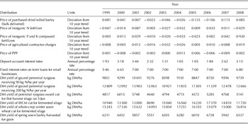
Fitting the deviation values to the current mean price (2010) for the input provides a stochastic price series that removes the deterministic trend but retains the stochastic fluctuation around the mean price level. Each constructed series provides the input parameters (states) necessary to establish a discrete probability distribution for that input price. The discrete price distributions simulated for each of the 10 years are shown in Table 2. The exceptions to this price series adjustment were interest rates, which tend to return to mean values rather than trend in a particular direction. Therefore, the discrete observed values were used for both deposit and loan interest rates.
Yield data
Production risk is defined for the purposes of the current study as the year-to-year yield variation of a feed crop, as a result of weather variation and unforeseen crop pests and diseases. Year-to-year variation also extends to variation in nutritional value of feed crops on a given farm. However, given the lack of consistent long-term nutritional value data and the fact that previous studies found that feed cost was more sensitive to variation in DM yield than nutritional value variation (Savoie et al. Reference Savoie, Parsch, Rotz, Brook and Black1985; O'Kiely et al. Reference O'Kiely, Moloney, Killen and Shannon1997), the stochastic analysis of production risk focused solely on DM yields for the purposes of the current study.
For this analysis, GFCM default yield calculations were overridden. The DM yields used were the 10-year (1999–2008 inclusive) control yields for feed crops from variety trials published by the Irish Department of Agriculture, Fisheries and Food (DAFF 2010). The time-period studied was limited to 10 years due to data access difficulties. These trials are conducted annually at seven locations throughout the Republic of Ireland to identify new feed crop cultivars suitable for commercial use. Control yields are calculated as the mean yields (over all sites) of two to three approved commercial cultivars for a particular year. Crop management procedures were maintained at a consistently intensive level across the cultivar testing locations and years. Technological changes to crop management practices were minimal over this time period. Thus, yield fluctuations could be reasonably attributed to year-to-year variation in weather and unforeseen pests and diseases. However, because the control cultivars for some crops were changed every 2–3 years during this period, it must be borne in mind that some element of the observed yield variation may be due to improved yields of new crop cultivars, as described by Talbot (Reference Talbot1984). As the variety trials did not include a low-nitrogen (N) grazed perennial ryegrass sward, the yields for the GG90 sward were predicted from the variety trial yields using the GFCM perennial ryegrass N response equation (Eqn (5)). The discrete 10-year yield distributions simulated for each of the seven feed crops are shown in Table 2.
where DMYGG is the annual dry matter yield (kg DM/ha) of grazed grass and N is the annual rate of fertilizer N applied (kg/ha).
Feed crop scenario analysis
The feed crop scenarios in terms of management and non-management factors are generally as described in the Appendix (available online at http://cambridge.journals.org/AGS). The scenarios were: a grazed grass sward receiving 90 kg inorganic N fertilizer/ha/yr (GG90), a grazed grass sward receiving 200 kg inorganic N fertilizer/ha/yr (GG200), two grass silage scenarios using different conservation technologies (GS, primary harvest perennial ryegrass bunker silage; GSB, primary harvest perennial ryegrass baled silage), a whole-crop maize (WCM) silage, a whole-crop wheat (WCW) silage, a BG crop and a purchased rolled barley feed (PRB). Table 3 illustrates the main management scenarios simulated for each of the eight feed crops in the stochastic analysis.
Table 3. Feed crop management scenarios and nutritional values simulated for stochastic analysis

* Sward age for perennial crops in years.
† kg/ha/year.
‡ g DM/kg.
§ g/kg DM.
** UFV/kg DM; GG90, grazed perennial ryegrass 90 kg N/ha; GG 200, grazed perennial ryegrass 200 kg N/ha; GS, primary harvest perennial ryegrass bunker silage; GSB, primary harvest perennial ryegrass baled silage.
GG90 and GG200 were perennial ryegrass swards rotationally grazed by cattle at a stocking rate of 110 and 170 kg organic N/ha, respectively. Stocking rate was defined as the annual organic N excreted by grazing livestock per grassland hectare, as defined by the Nitrates Directive (Anonymous 2006). Fixed costs were constant for the two grazed grass swards (Table 5). The grass silage crops (GS and GSB) had a final spring defoliation date of 31 March and were mowed for silage on 15 May. GS was consequently harvested by a precision-chop forage harvester following a 6 h wilt. GSB was wilted in situ for 48 h before baling and wrapping. WCM was sown in late April without the use of polythene mulch. The whole-crop silages and the BGs were all assumed to be sown, managed and harvested at dates deemed most favourable for achieving optimal maturity for the specified harvesting and conservation options (i.e. fermented whole-crop silage for the wheat and maize, and propionic acid treatment for the BG). Fertilizer application rates for all crops were based on the requirements for Irish conditions specified by Coulter & Lalor (Reference Coulter and Lalor2008). The default purchased feed included as a benchmark for the home-produced feeds in the current analysis was dried, rolled BG, purchased and delivered at a mean price of €170/t (CSO 2010a). The purchased rolled barley price was included as a stochastic variable to quantify the effect of feed market supply and demand on feed cost risk. For the stochastic analysis, all feed cropping scenario parameters except for DM yield and unit price of inputs were assumed to remain constant. All stochastic variables were simulated simultaneously with input variables correlated according to the 10-year dataset (Table 4). There was a strong positive correlation between the price of P and K and N fertilizer, between GG90 and GG200 DMY and between WCM and BG DMY. The main default costs for each of the eight feeds are shown in Table 5. For further detail on the crop assumptions, functions and default parameters please refer to the Appendix (available online at http://cambridge.journals.org/AGS).
Table 4. Correlation coefficients for stochastic model input variables based on 10-year discrete distributions

* Feed codes as per Table 3.
DMY, dry matter yield.
–=Negligible (>−0·30 and <0·30) or zero correlation.
Table 5. Mean feed costs €/ha (except where otherwise stated)
Feed crop codes as per Table 3.
† Fertilizer cost includes contractor spreading cost.
‡ PPP cost includes contractor spraying cost.
§ Contractor cost includes crop establishment, harvesting, processing and feed-out operations as well as herding cost for the grazed scenarios.
** Fixed costs include depreciation of fixed assets, including sward establishment and fencing costs for grass crops and storage facility costs for harvested crops.
†† TFC includes LC of €300/ha/yr.
‡‡ Purchased rolled barley costs expressed as €/t utilized dry matter; mean purchase price €170/t fresh grain delivered.
RESULTS
Mean cost
With mean TFC expressed on a net energy basis, the feeds ranked from least to most expensive: GG200, GG90, PRB, BG, WCW, WCM, GSB and GS (Table 6). GG200 was the cheapest feed crop at a mean cost of €74/1000 UFV. The more extensively stocked GG90 was 7% more expensive, while the conserved feeds ranged from 254% (PRB) to 291% (WCM) of the cost of GG200. PRB was the least expensive alternative to grazed grass over the 10 years, and was 2·5% cheaper than the home-produced barley.
Table 6. TFCs (€ 1000/UFV) stochastic analysis results

* Feed codes as per Table 3.
s.d., standard deviation; CV, coefficient of variation.
Total risk
The CDFs in Fig. 3 indicate the level of TFC risk for each of the eight simulated feeds over the period 1999–2008. Flatter CDFs imply greater riskiness, steeper curves indicate less risky feeds. CDFs to the left are preferred (lower TFC). Some of the CDFs to the right intersect one another, suggesting that the preferred choice among these would depend on the level of risk averseness of the decision maker. Using coefficient of variation (CV) as a measure of total riskiness, the feeds ranked BG, PRB, WCW, GSB, GG90, GG200, GS and WCM from lowest to highest risk (Table 6). The most expensive example of GG200 (95th percentile) was €71/1000 UFV less expensive than the cheapest alternative to GG: a high-yielding WCM crop under a scenario of low input prices (5th percentile) (Table 6). At the 5th percentile WCM was also the only conserved feed that was less expensive than PRB. However, at the 95th percentile, WCM was the most expensive feed. BG exhibited the lowest total risk (CV 0.063), just below that of PRB (CV 0·064), which incurred no direct exposure to yield risk.
Price risk
The feeds least sensitive to price risk were GG90, GG200, WCW and BG (Table 6). The feeds most sensitive to input price fluctuations were PRB, GS and GSB. PRB was most sensitive to the market price of rolled barley because purchase price comprises 0·895 of PRB TFC. The greatest component of total price risk was P and K price, generally followed by contractor price, and then N price, for all home-produced feed crops except for GG90 and GG200, which were more sensitive to N than contractor price (Table 7). All the feeds exhibited low levels of sensitivity to price risk of the other inputs examined (namely PPP price, deposit interest rate and loan interest rate).
Table 7. Regression coefficients for TFC against input price risks and yield risk

* Feed codes as per Table 3.
DMY, dry matter yield.
Yield risk
Yield variability was the greatest risk affecting TFC of the seven home-produced feeds in the current analysis (Tables 6 and 7). The feeds least sensitive to yield risk were GSB and BG. Both feeds incur a high proportion of yield-dependent costs within TFC. All bale-related costs (baling, wrapping and handling) are a direct function of yields, and similarly the substantial rolling and propionic acid treatment of BG are costed on a per tonne basis. Conversely, high proportions of fixed costs and area-dependent variable costs within TFC can increase the exposure to yield risk because lower-than-average yields result in considerable ‘under-capacity costs’ (Shoup Reference Shoup, Shoup and Peart2004). The feeds most sensitive to yield risk were GG90, GG200 and WCM.
DISCUSSION
Mean TFC relativity
As expected, the greater yields of grass utilized under the GG200 scenario than the more extensive GG90 scenario resulted in a lower mean cost per unit net energy for GG200. The lower feed cost was achieved via increased stocking rate and N application, because the area-dependent LC and fixed costs were diluted by the greater output.
Grazed perennial ryegrass was, as expected, the cheapest feed in the analysis. However, its production is seasonal and utilization is poor during periods of soil waterlogging. To address this imbalance, it has been proposed that grass should be costed as a ‘full-year feed’ by including the cost of a conservation harvest required to feed a proportion of the grazing livestock over the following winter (Finneran et al. Reference Finneran, Crosson and Wallace2010a). Taking conservation harvests during the period of peak summer grass production is an aid to good grassland management because surplus grass is not wasted. This complementary benefit to grazed grass of a conservation harvest should be acknowledged when comparing the cost of grass silages with other conserved feeds. Further GFCM studies will address this issue.
The substantial cost advantage of grazed perennial ryegrass and its predominance in pasture-based ruminant production systems dictate that it is beneficial to express the cost of alternative feeds relative to the cost of grass. The relative cost of grain feeds to grazed grass was lower in this analysis than that found by O'Kiely et al. (Reference O'Kiely, Moloney, Killen and Shannon1997). However, the relative costs of silages (grass, wheat and maize) to grazed grass were very similar in both studies.
As a result of the greater contractor and total costs per hectare associated with baled grass silage relative to a bunker-ensiled grass crop (Table 5), it was somewhat surprising that GSB was on average cheaper than GS for the 10 years’ yields simulated. This lower cost for GSB is mainly due to two factors. Firstly, GSB incurs a relatively low proportion of fixed costs and area-dependent variable costs, because most costs are incurred on a ‘per bale’ rather than a ‘per hectare’ basis. In contrast, harvesting costs for GS are area dependent and fixed costs are greater, due to the use of concrete silos. Secondly, because bales are wrapped and fed out individually, greater DM conservation and feed-out efficiencies are attributed to bales relative to bunker silages. The combination of these factors appears to more than offset the additional harvesting and feed-out cost of bales at the mean yield in the current analysis. Previous work has shown that at higher mean yields (>6 t DM/ha), the fixed costs and area-dependent costs of a bunker-ensiled crop are diluted to the extent that bunker silage becomes a less expensive technology than bales (Finneran et al. Reference Finneran, Crosson, O'Kiely, Shalloo, Forristal and Wallace2010b).
Maize silage and wheat silage were 4 and 5% less expensive on average than grass silage. This provides some explanation for the increase in area of these whole-crop silages over the past decade in Ireland (CSO 2010b). This increase is likely to be due to a combination of the mean cost advantage of wheat and maize silages and farmer perceptions of the differing risk factors affecting each of these feeds as discussed below.
The lower mean cost of purchased barley relative to the home-produced BG suggests an element of market failure for feed barley producers in Ireland, in that the market price did not meet the production cost of BG over this time period. This shows that on average, for the assumptions used in this analysis, BG was more expensive to grow than to purchase. This mirrors the results of optimization modelling by Neal et al. (Reference Neal, Neal and Fulkerson2007), which often favoured the purchase of cereal grains over home production in Australia.
TFC risk
As illustrated in Fig. 3, WCM exhibited the maximum risk of any of the feeds in this analysis. This is not unexpected in that maize is a relatively new crop to Ireland and until recently, climatic conditions had been described as marginal for maize (Crowley Reference Crowley2005). In recent years, new cultivars have been developed that mature earlier, requiring fewer heat units to reach maturity, peak cob and whole-crop yields. Consequently, yields have been increasing at a greater rate for maize than for any other crop in the national variety testing programme over the past 10 years. Therefore, some of the ‘yield risk’ (e.g. above the 60th percentile; Fig. 3) attributed to maize in this analysis may be a reflection of the inherently lower-yielding cultivars sown in the earlier part of the decade studied. In addition, the technology of sowing maize under polythene film is now widespread in inland and northern regions of Ireland and has significantly increased whole-crop yields (Crowley Reference Crowley2005). This technology could not be simulated in the current analysis as no polythene-covered plots were included in the variety trials for the first 5 years of the time period analysed for the current study. Therefore, the maize yields used for the current analysis were from crops sown without plastic cover. The wide range of TFC values observed for maize meant that it could be both the cheapest alternative to grazed grass (at the 5th percentile), and the most expensive (at the 95th percentile; Fig. 3). Therefore, the level of risk that an individual farmer could tolerate would be a key factor if making a decision between planting maize or an alternative crop.
WCW and WCM maintained very similar mean costs in the current analysis (Table 6). On average, WCM was 1·1% more expensive than WCW. However, WCM exhibited a TFC CV of 19·5 as against 0·067 for WCW, primarily due to the greater yield risk incurred by the maize crop. The higher yield risk of WCM is due to the greater weather risk associated with maize than wheat, because of the inherent greater heat unit requirements for the maize plant to attain maturity. These results maintain similar relative yield variability values to those documented by Talbot (Reference Talbot1984), who reported CV values of 0·18 and 0·26 for wheat and maize yields respectively, using 13 years variety trial data in the UK. Wheat cultivars have been selected for suitability for Irish conditions for a much longer time period than maize and consequently technological improvements in management and genetics have improved both yield volume and yield consistency over many years. Therefore, the increasing area sown for WCW and WCM in recent years in Ireland may be due to the relative consistency of yields for wheat, and the high yields of maize achievable under favourable weather conditions and the use of newer, higher-yielding cultivars and/or polythene mulch technology.
As a technology for ensiling primary harvest perennial ryegrass, GS is less expensive than GSB below the 20th percentile because while the yield-dependent TFC of GSB is advantageous at lower yields, at yields greater than 5·7 t DM/ha (such as observed in 2000 and 2001; Table 3), the more area-dependent GS is the cheaper option. At lower GS yields, the fixed cost of the concrete bunker and the area-dependent contractor charge for harvesting greatly increase TFC per unit of feed due to the problem of over-capacity. The reduced yield risk factor associated with GSB relative to GS partially explains the increasing popularity of an apparently more expensive feed (GSB) in Ireland in recent years.
BG was the least risky feed in the current analysis (Table 6), due in part to the yield-dependent conservation and feed-out costs discussed above and also the lowest yield variability of any of the harvested crops. This is in agreement with the work of Talbot (Reference Talbot1984), who noted that low-yield variability was a feature of lower-yielding crops such as spring barley.
Perhaps the most striking of all the results is the fact that, besides being the least expensive alternative to grazed grass at mean cost, PRB also exhibited a relatively low level of TFC risk. While WCM was less expensive than PRB below the 35th percentile, the overall CV value of PRB was lower than that of any home-produced feed except for BG. This leads one to the conclusion that greater TFC risk is incurred by growing feeds than by purchasing them on the open market. The cost of PRB, being a more stable, energy-dense feed and therefore suited to prolonged storage and international trade, is understandably less sensitive to domestic price and yield risks than the other less stable or tradable feeds in this analysis. Although rolled barley cannot be fed as the sole component of a ruminant diet, it is generally a primary constituent of concentrate feed mixes. It appears that, assuming feed trading prices maintain the trend of the past decade, purchase rather than growing of conserved feed could be the most effective risk reducing strategy for a ruminant livestock farmer. However, purchased feed prices have become much more variable in recent years (2006–2010; CSO 2010a) and this market volatility will be the key factor in determining the relative riskiness of purchasing rather than home production in the future.
General implications
Risk quantification is an important consideration for farmers assessing a feeding strategy decision. The following discussion points highlight some of the most important considerations when deriving farm-level implications from the results of this analysis.
1. The time period examined in the current analysis included the commodity price spike in 2007/08. The considerable increase in P and K fertilizer price from 2007 to 2008 (Table 3) represented an inflation rate 36 times greater than that observed over the previous 10 years (1998–2007). In spite of this, yield risk was of a much greater magnitude than input price risk for all feed crops over the time period examined (Table 6). This result had been indicated but not quantified by the findings of previous authors (Savoie et al. Reference Savoie, Parsch, Rotz, Brook and Black1985; Coyle Reference Coyle1992; O'Kiely et al. Reference O'Kiely, Moloney, Killen and Shannon1997; Neal et al. Reference Neal, Neal and Fulkerson2007). Therefore, although input price volatility has increased during the past decade (CSO 2010a; USDA 2010), yield remains the key variable driving feed crop cost and risk.
2. The yield distributions used in the current analysis were obtained from intensively managed trials in multiple locations and enjoying a high level of management input. It can therefore be assumed that on more extensively managed, single-location farms, inter-annual yield variability would be much greater than that observed in the aggregated time series distributions used here (Coyle Reference Coyle1992; Just & Weninger Reference Just and Weninger1999; Rudstrom et al. Reference Rudstrom, Popp, Manning and Gbur2002). This implies that greater TFC ranges for all feed crops would occur on individual farms relative to the national mean values presented in the current analysis.
3. The price and yield variation simulated represented the ‘unpredictable and uncontrollable’ elements of feed crop TFC. They were defined using data collected at a national level. At individual farm level ‘extreme’ risks such as fires, prolonged droughts or flooding would pose significant but rare risks to feed crop TFC. These risks were beyond the scope of the current study but could be accounted for using an approach such as that used by Mosnier et al. (Reference Mosnier, Agabriel, Lherm and Reynaud2009), who quantified the risks of large yield and price shocks for suckler beef systems in France.
4. Because contractor charges were assumed for all cropping and feed-out operations, farms using owned machinery may incur lower variable costs than those quoted in the current paper. The two main problems that may arise when using owned machinery, as described by Shoup (Reference Shoup, Shoup and Peart2004), are machinery over-capacity resulting in fixed cost inefficiencies and under-capacity resulting in timeliness-related crop losses. Complex machinery assumptions relating to cost, age, work rate and efficiency are avoided by assuming contractor use for all operations. However, the assumption that no timeliness-related crop losses occur when using a contractor is questionable (Gunnarsson et al. Reference Gunnarsson, Spörndly, Rosenqvist, de Toro and Hansson2009).
5. On individual farms, multi-cropping is commonly practised, whereby multiple feed crops are grown in any one year, thereby distributing annual feed cost risk across the different crops. However, while such a strategy would reduce TFC risk at whole-farm level, the level of risk reduction is limited because, as the results of the current study showed (results not presented) TFC risk was strongly positively correlated across the home-produced feed crops.
6. The main assumption underpinning the stochastic analysis is that previously observed prices and yields are a reasonable guide to current or future values. This assumption can be reasonably well defended as regards crop yields, with the noted allowances made for technological improvements. Crop yields are unlikely to decrease in the absence of widespread disease or pest problems or unfavourable changes in climate, and unlikely to increase in the absence of technological changes. However, the assumption that historic price variability can serve as a guide to future price variability may be less robust. Recent periods of rapid energy price inflation followed by deflation have added uncertainty to the challenge of predicting future price risk (USDA 2010).
CONCLUDING COMMENTS
As livestock production systems also involve numerous sequential processes following on from the production and utilization of the feed, and each with their own cost and risks, whole-farm analysis would be the most appropriate technique to evaluate and compare home-produced feeds. Ideally, feed cost would be expressed per unit of product; e.g. beef, milk, etc. The feed cost and risk information derived from the use of the GFCM can form a valuable input to such a whole farm analysis exercise.
The current study has indicated some management strategies that can be employed to minimize exposure to the uncontrollable risks posed by unfavourable weather and unforeseen pests and diseases. The analysis has shown that those feed crops requiring investment in fixed facilities incur greater exposure to yield risk than feed crops incurring a lesser proportion of fixed costs (e.g. GS v. GSB). The substantial cost advantage of grazing as a means of feed utilization is highlighted by the relatively low cost of grazed grass in the current study.
The finding that purchased rolled barley was the least expensive and also a low-risk alternative to grazed grass raises questions as to the economic logic for home production of conserved feeds when input price and yield risk are considered. It could be inferred from these results that a ruminant livestock farmer could have reduced exposure to feed cost risk by purchasing BG, thereby transferring the greatest burden of risk to the barley producer. It remains to be seen how this dynamic will change under future global scenarios of growing animal and human feed demand and increasingly volatile energy prices.
The GFCM is unique as a powerful analytical tool to examine the interactions of biological, management and market factors on feed crop cost. Risk quantification through the use of stochastic analysis in the model strengthens the GFCM outputs by indicating the relative sensitivity of the different feed crops to the various risk factors outside the control of an individual farmer. Multiple feed crop production, utilization and economic datasets have been brought together, permitting a novel quantification of the complex dynamic relationships constantly evolving between the farmer, technology and economic and biological risk.
SUPPLEMENTARY MATERIAL
The appendix is available online as supplementary material at http://journals.cambridge.org/AGS
The authors acknowledge the financial support of Walsh Fellowship funding to E. Finneran. The authors would also like to thank D. Grogan, B. O'Reilly and the staff of the Irish Department of Agriculture, Fisheries and Food for providing the crop yield data.


