


Introduction
The distribution of the number of secondary transmissions per single primary case, i.e. offspring distribution, of severe acute respiratory syndrome coronavirus 2 (SARS-CoV-2) has been described as being overdispersed, and this has been a well-known feature of the coronavirus disease 2019 (COVID-19) pandemic [Reference Lau1–Reference Chen3]. The majority of primary COVID-19 cases generate no or only a small number of secondary causes, whereas only approximately 10–20% of SARS-CoV-2-infected individuals contribute to causing 80% of secondary COVID-19 cases [Reference Endo4–Reference Miller7]. Published epidemiological evidence indicates that those transmissions have been caused mostly by super-spreading events (SSEs) [Reference Lloyd-Smith8], i.e. an event at which an unusually high number of secondary cases was produced by a single primary case [Reference Park9, Reference Muller10].
An in-depth understanding of individual-level variations in COVID-19 secondary transmission is essential for designing a customised COVID-19 control strategy [Reference Nielsen, Simonsen and Sneppen6]. Considerations of overdispersion actually influenced the contact tracing practice in Japan, which assumed that if intervention efforts focused on contact tracing and minimising the chance of SSEs (i.e. targeted high-risk settings that may lead to large numbers of secondary transmissions), it might be possible to efficiently bring the epidemic under control [Reference Jung11–Reference Wong and Collins14]. Indeed, a ‘backward’ (or ‘retroactive’) method of contact tracing, in which both the new secondary cases and the primary cases from whom they originated are traced, was implemented during the early stages of each epidemic wave in Japan, with the aim of identifying the dominant source of SSEs and calling for secondary transmission preventions in such settings [15, Reference Oshitani16]. Secondary transmission events, especially SSEs, were found to be more likely to occur in specific circumstances with the ‘3Cs’ (close contacts in a closed environment with crowded conditions). Accordingly, by implementing public health and social measures that focused on high-risk settings with the 3Cs features (e.g. closing host and hostess clubs, shortening opening hours and restricting the maximum number of customers per table in dining service), the second wave of the COVID-19 epidemic was suppressed without implementing a lockdown of the entire community [Reference Jung11]. However, relying solely on such a focused intervention strategy, specifically concentrating on prevention in high-risk settings, was insufficient to control the epidemics in the later waves.
Japan experienced larger epidemic waves of COVID-19 after the second wave, leading to calls for the declaration of a state of emergency (SoE) and the enactment of more stringent countermeasures. The failure to effectively suppress these waves may be a consequence of the delayed initiation of appropriate countermeasures (e.g. when customised interventions were in place, the transmission was taking place in broader community settings, including households and workplaces). However, it is also possible that variations in the number of secondary transmissions may have occurred as a result of the emergence of SARS-CoV-2 variants of concern with elevated transmissibility, including the Alpha (B.1.1.7) and Delta (B.1.617.2) variants. Thus, to continue with our case isolation and contact tracing efforts during the waves caused by these variants, we faced the need to devise a method for monitoring the overdispersion of offspring distribution, so that we could judge whether focused interventions were still justified.
Conventionally, individual-level variations in the offspring distribution have been quantitatively measured by the dispersion parameter (k) of a negative binomial distribution, with lower values of k corresponding to a broader (more skewed) distribution [Reference Endo4, Reference Sneppen17]. However, estimating overdispersion from empirical contact tracing data has been very challenging in practice for the following two reasons. First, cases causing large clusters are more likely to be detected than are cases causing only a small number of secondary transmissions. However, a large number of transmissions occurring in a public setting (e.g. public transportation) might not be more ascertained compared with household transmissions, which tend to be investigated with the highest priority during contact tracing. As a result, the naïve estimation of k made by relying solely on observed data might be affected by ascertainment bias from both directions. Second, in a real time evaluation, a subset of the secondary cases infected by the recently reported cases would not have been observed yet in the surveillance system owing to the censoring of observational time, resulting in an underestimated number of secondary transmissions. Here, to examine the time-dependence in the variations in the number of secondary transmissions, we quantitatively examined the overdispersion parameter using empirical contact tracing data from two waves of the COVID-19 epidemic in Japan. We explored the second and fourth waves when the ancestral and the Alpha variants of SARS-CoV-2 were dominant, respectively, to account for the abovementioned ascertainment bias and right censoring.
Methods
Transmission data
To explore variations in the number of secondary transmissions of SARS-CoV-2, information on the confirmed COVID-19 cases during ‘wave 2’ from 12 July to 21 September 2020 and ‘wave 4’ from 5 March to 12 April 2021 in Nagano Prefecture was retrieved from the prefectural government website [18]. Among the 47 prefectures in Japan, Nagano was specifically selected because it has publicly released detailed individual-level data, including information regarding the transmission link, i.e. from whom the infection was acquired, in a timely manner. The study periods in Nagano were selected to ensure that the transmission dynamics of COVID-19 during the study periods were not affected by stringent countermeasures, such as a prefectural- or national-level SoE. For this reason, the third wave was excluded from our study (the majority of the third wave was accompanied by a SoE in response to the upsurge of cases), and only the early phase of the fourth wave was analysed.
A COVID-19 case was defined as any COVID-19 case confirmed by reverse transcriptase polymerase chain reaction (RT-PCR) for SARS-CoV-2, regardless of symptoms. Consequently, asymptomatic infections that were associated with contact tracing were included in our data. From the 1083 reported COVID-19 cases, the 572 cases for which their infector information was identified via contact tracing were extracted. The infector–infectee pairs were categorised into two types: (1) household transmission pairs, and (2) non-household transmissions pairs. Infectees who had multiple potential infectors, i.e. cases with inconclusive multiple primary cases, accounting for <5% of all infectees (28/572), were excluded. Infectors were aggregated into the following three age groups: 20–39, 40–59 and ⩾60 years old. Individuals aged less than 20 years old were not included in our age-dependent analysis because the sample sizes from our selected observation periods were too small (there were 0 and 5 primary cases in children during waves 2 and 4, respectively).
Statistical analysis
Estimation of the reproduction number (R) and overdispersion parameter (k)
We fitted the negative binomial distribution to empirically observed offspring distributions. The probability mass function of the negative binomial distribution was calculated as

where x is the number of secondary cases generated by a single primary case. R and k are parameters representing the mean and dispersibility of the negative binomial distribution, respectively. The mean of the negative binomial distribution, by definition, is referred to as the reproduction number. Considering the effect of stringent interventions enacted in the latter part of wave 4, the majority of the wave 4 data collected for this study were from the ascending phase of the wave, whereas the wave 2 data collected were from throughout the entire wave (i.e. both the ascending and declining phases of the wave). Thus, to identify any potential bias caused by using data from different epidemic phases, we also estimated the R and k using only the ascending epidemic phase data of wave 2 (see Sensitivity analysis using the ascending epidemic phase data of wave 2 in Supplementary material).
Because an ascertainment bias influences the observed number of primary cases who did not contribute to secondary transmission at all (e.g. sporadically occurring cases are less likely to be detected/diagnosed compared with cases involved in a larger cluster), we analysed both zero-included and zero-truncated data to check the sensitivity of our results for an ascertainment bias [Reference Farrington, Kanaan and Gay19]. The following likelihood functions used for the zero-included and zero-truncated data were formulated:


respectively, where X = {x 1, x 2, …x N}, and N is the sample size.
Schematic drawings of the methods used to control right-censored infection trajectory chains during a real time assessment. To control right-censored data, two methods were applied (see Right censoring adjustment for infection trajectory chain in Methods). (a) Exclusion of all potentially censored data: infectors whose secondary cases are potentially unobserved (black circles in the light blue-shaded area) were excluded from the analysis (method 1). The 97.5th percentile of the time delay from the reporting of a primary case to that of the secondary case (report–report time), i.e. 9 days, was used for the exclusion period. (b) Likelihood adjustment for censoring: an adjusted likelihood function (Equation (4)) for the number of secondary cases was used for the analysis (method 2). Infectors in the light blue-shaded area (3 days, i.e. the median of the report–report time, from the cut-off date) were excluded for this adjustment. T, data cut-off date; t 1, date of the report of case #1; t 2, date of the report of case #2; t3, date of the report of case #3.

Right censoring adjustment for infection trajectory chain
During a real time assessment, as well as here because we truncated the epidemic curve of wave 4 and considered only the time period without a SoE declaration, the trajectory chain is right-censored (i.e. cases that occur close to the cut-off date are likely to have missing infectee information; Fig. 1). To overcome this problem, we applied the following two methods.
(1) Exclusion of all potentially censored data: infectors whose secondary cases were not fully observed owing to censoring (primary cases in the shaded area in Fig. 1a, i.e. generation time was not completed) were excluded from the analysis. The 97.5th percentile of the time delay from the reporting of a primary case to that of the secondary case (the report–report time distribution), i.e. 9 days from the latest calendar time, was determined as the cut-off point for exclusion.
(2) Likelihood adjusted for censoring: All observed data were included, and the likelihood function was adjusted using the report–report time distribution (see below).
For method (2), we used the empirically observed number of secondary cases for primary case i, xi (number of blank circles drawn by a solid-line in Fig. 1b), adjusting it for right censoring. We set ti as the time at which primary case i is reported and T as the cut-off date in the calendar time. The likelihood function for the entire dataset (i.e. the non-excluded data) is


where Y = {y 1, y 2, …y N > 0}, ⌊.⌋ is a floor function (thus, Equation (5) indicates we rounded $x_i/\mathop \smallint \nolimits_0^{T-t_i} g( t ) dt$ to the nearest integer), and g(.) is the probability density function of the time from reporting in a primary case to that in the secondary case. The data from the most recent 3 days before the cut-off date were excluded (light blue-shaded area in Fig. 1b) because the adjustment was unreliable owing to the very small values of g(.). The timespan of 3 days corresponded to the median length of the report–report time.
Offspring distributions for household and community settings
Subsequently, we divided all reported transmissions into the following two types according to their place of transmission: household and non-household. We then compared the following three features between wave 2 and wave 4: (1) the proportion of household transmission, (2) the proportion of people whose number of secondary cases was >5 (i.e. those who caused an extraordinarily large cluster) in non-household settings, and (3) the average number of secondary cases infected by a single primary case in each setting. These comparisons between waves 2 and 4 were conducted using the two-sample test for equality of proportions and the Wilcoxon rank-sum test. Potentially censored infectors were excluded for these analyses as well, and the sample sizes used were 107 and 310 pairs for household and non-household transmission, respectively.
Results
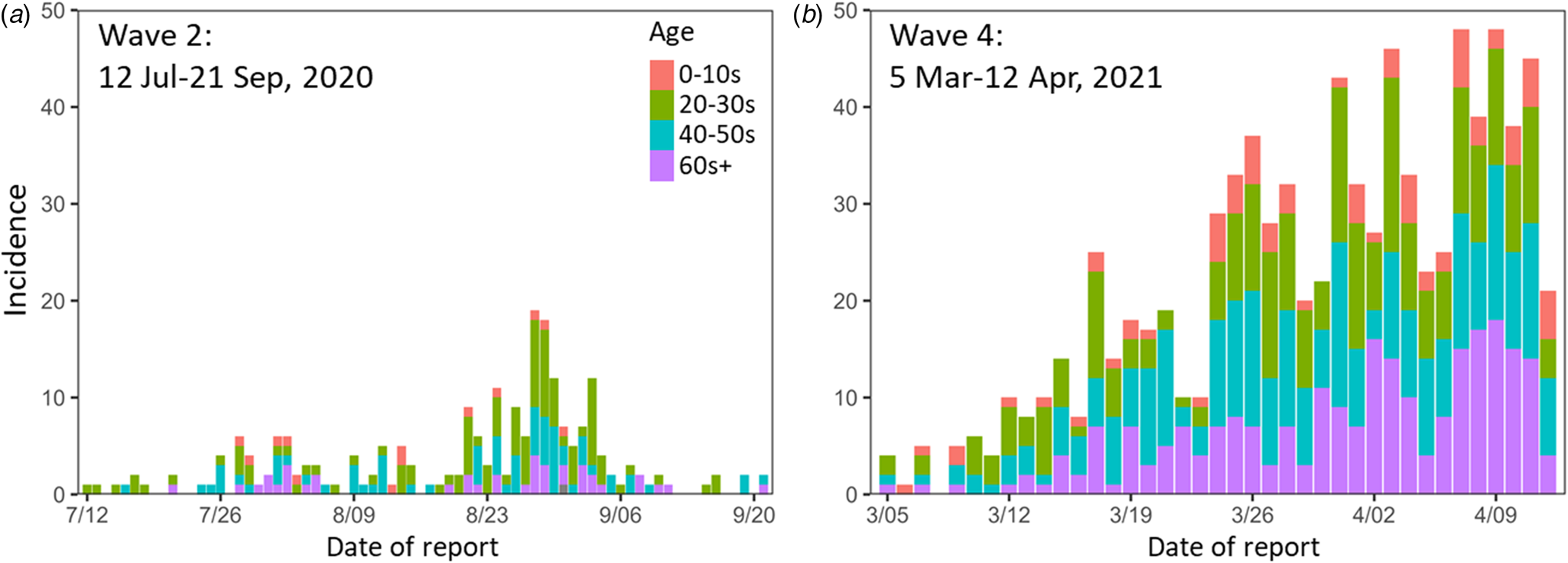
The epidemic curves for the newly reported COVID-19 cases during the study periods in Nagano are shown in Figure 2. The empirically observed offspring distributions, stratified by the epidemic period and age group, that were used for the estimations of R and k are shown in Figure 3. All observed distributions were right skewed across all age groups.
Epidemic curves for the study periods. (a) Wave 2 (12 July–21 Sep 2020). (b) Wave 4 (5 Mar–12 Apr 2021). Colours indicate age groups. Wave 2 contains one case of unknown age.
Observed epidemic period- and age-dependent offspring distributions. (a, e) Epidemic period-dependent offspring distributions for waves 2 (a) and 4 (e). (b–h) Age-dependent offspring distributions for age groups: 20–39 (b, f), 40–59 (c, g) and ⩾60 years old (d, h) of waves 2 (b–d) and 4 (f–h).

Estimated dispersion parameter, k, for a negative binomial distribution
Our estimates of R and k are shown in Table 1. In both the analysis conducted with the zero-included data and that conducted with the zero-truncated data, the dispersion parameter, k, was estimated to be greater for wave 4 than it was for wave 2 (although the absolute values of k were not necessarily consistent), suggesting that the dispersion of the number of secondary transmissions of SARS-CoV-2 by a primary case had decreased in wave 4. The age-dependent analyses yielded a different trend between the analysis with the zero-included data and the analysis with the zero-truncated data. The former found smaller k values for older age groups, and this age-dependence was consistent for both epidemic waves (waves 2 and 4). The latter, in contrast, found the highest value of k for individuals aged 20–39 years and the lowest estimate of k for those aged 40–59 years. The likelihood that addressed right censoring led to estimates that were overall in good agreement with the simple method that further truncated and excluded the empirical data.
Estimated dispersion parameter, k. Parameter estimations (for reproduction number, R and k) were performed for the zero-included and zero-truncated offspring distributions

a Right-censoring data excluded from the analysis.
b Right-censoring data adjusted for the analysis (see Right censoring adjustment for infection trajectory chain in Methods).
Offspring distributions plotted using the parameters (R and k) estimated from the model produced with the zero-included data are shown in Figure 4. The offspring distribution of wave 2 was more skewed than that of wave 4, and the probability of being a zero-secondary-case (i.e. one for whom the number of secondary cases was zero) was higher in wave 2 (Fig. 4a). Regarding age-dependent offspring distribution, the older age group showed greater overdispersion (i.e. a smaller value of k) compared with the younger age group (Fig. 4b). This age-dependence was consistent between waves 2 and 4 (Fig. 4c and d). To examine the fitness of the estimations, the estimated offspring distributions were overlaid with the observed data, and the modelled distribution visually appears to have effectively captured the observed patterns of the data (Figs S1 and S2).
Estimated epidemic period- and age-dependent offspring distributions for the zero-included data conducted using the censoring data exclusion method (method 1 in Right censoring adjustment for infection trajectory chain in Methods). (a) Epidemic period-dependent analysis. (b) Age-dependent analysis for the entire epidemic period (both waves 2 and 4). (c–d) Age-dependent analyses for waves 2 (c) and 4 (d).

The offspring distribution determined from the zero-truncated data was also visualised (Fig. 5). The qualitative patterns among the analyses of the zero-truncated data were similar (Figs 4a and 5a). The group of individuals aged 40–59 years showed the most skewed distribution, and those in this group had the highest probability of being a zero-secondary-case (Fig. 5b and d). As the two adjustment methods for censoring produced consistent results for the estimated parameters, they likewise yielded offspring distributions that were visually consistent (Fig. 5a–d). The estimated offspring distributions overlaid with the observed data are shown in Supplementary Figures S3 and S4.
Estimated epidemic period- and age-dependent offspring distributions for the zero-truncated data. (a) Epidemic period-dependent analysis conducted using the censoring data exclusion method (method 1 in Right censoring adjustment for infection trajectory chain in Methods). (b) Age-dependent analysis for the entire epidemic period (both waves 2 and 4) conducted using the censoring data exclusion method (method 1 in Right censoring adjustment for infection trajectory chain in Methods). (c) Epidemic period-dependent analysis conducted using the censoring data adjustment method (method 2 in Right censoring adjustment for infection trajectory chain in Methods). (d) Age-dependent analysis for the entire epidemic period (both waves 2 and 4) conducted using the censoring data adjustment method (method 2 in Right censoring adjustment for infection trajectory chain in Methods).

Variations between household and non-household settings
To explore if the disease transmission settings influenced the variation in offspring distribution between waves 2 and 4, a descriptive analysis was performed for transmission settings (i.e. household and non-household settings) (Supplementary Fig. S5). The proportion of secondary transmissions that were household transmissions was higher in wave 4 (32.6%, 102/313, P < 0.001) than in wave 2 (4.8%, 5/104). In the non-household setting, the proportion of primary cases who contributed to generating more than five secondary cases was not different between wave 2 and wave 4 (P = 0.838), indicating that SSEs were observed at the same proportion in both periods (Table 2).
Descriptive analysis of offspring distributions for household and non-household settings

a The proportion of household transmissions among all transmissions.
b The proportion of people whose number of secondary cases was >5.
Discussion
To understand time- and age-dependent variations in the number of secondary transmissions of SARS-CoV-2 originating from a primary case, we investigated the COVID-19 contact tracing data from Nagano Prefecture, Japan. We found that the Alpha variant epidemic yielded less overdispersed results compared with the ancestral SARS-CoV-2 epidemic. The extent of dispersion may have been diminished as a more transmissible variant emerged.
Our analysis of the zero-truncated data produced a larger R compared with our analysis of the zero-included data. The estimate of R is influenced by the observed number of primary cases who did not contribute to secondary transmission at all, which may be biased by: (a) sporadically occurring cases, which are less likely to be detected (i.e. simply missing a lot of zeros from the empirical offspring distribution) and (b) cases who do not cause any secondary transmissions owing to quarantine, which are more likely to be included (i.e. including a lot of zeros because of interventions). Thus, the estimated R was different depending on the data type (zero-included vs. -truncated).
Our time-dependent analysis results indicate that the offspring distribution of wave 4 is less dispersed than that of wave 2. In general, an overdispersion of offspring distribution indicates a high frequency of SSEs [Reference Lloyd-Smith8]. However, the SSE frequencies were not different between waves 2 and 4 (P = 0.838), and what affected such variation was the lower frequency in wave 4 of primary cases who generated no secondary cases. This phenomenon is expected to occur when a variant that is more transmissible (on average) but less inherently variable in terms of infectiousness appears, and its occurrence here could be partly explained by the emergence of a more transmissible SARS-CoV-2 variant [Reference Davies20, 21]. Indeed, the Alpha variant was prevailing in Nagano during wave 4 [22], and a higher frequency of household transmissions was observed for wave 4 than for wave 2 (P < 0.001), suggesting that the less-dispersed offspring distribution observed for wave 4 could be a consequence of the invasion of the Alpha variant. A simulation study [Reference Nielsen23] also suggested that a SARS-CoV-2 variant that leads to less-dispersed secondary transmission would have an advantage over other variants under the conditions created by our response to the pandemic, i.e. using non-pharmaceutical interventions, including wearing masks, and/or regular testing, contact tracing and quarantining. Another potential factor could be changes in the COVID-19 risk awareness and human mobility patterns of a population. A search conducted using Google regarding human mobility relating to ‘retail and recreation’ in Nagano showed slightly higher values for wave 4 than for wave 2 [24]. Given that this category (retail and recreation) likely represents human mobility in the close-contact settings associated with SARS-CoV-2 transmission [Reference Jung25], such an increase in human mobility might have contributed to the decreased probability of primary cases who generated no secondary cases that was observed for wave 4. As a consequence of this decrease in the overdispersed secondary transmission of COVID-19 over time, the effectiveness of contact tracing and interventions focused on high-risk settings may be diminished [Reference Endo4, Reference Nielsen, Simonsen and Sneppen6, Reference Sneppen17], thus necessitating more intensive interventions to control the COVID-19 epidemic.
The time-dependent analyses for both the zero-included data and zero-truncated data produced consistent trends, showing that the offspring distribution was less dispersed when the Alpha variant was spreading. The surveillance system is affected by ascertainment bias, and larger clusters are more likely to be detected in the community, contributing to overestimation of the dispersion parameter [Reference Farrington, Kanaan and Gay19]. However, the under-ascertainment of sporadic cases contributes to the underestimation of the dispersion parameter because the probability of generating zero secondary cases would be erroneously estimated as smaller. In the case of wave 4, because the number of cases was higher than that in wave 2 (Fig. 1), larger clusters would be detected more often. Also, the increased number of SARS-CoV-2 tests conducted in wave 4 as compared with that in wave 2 [26] could have contributed to detecting a greater number of asymptomatic and mild cases via contact tracing. Despite these influences, our analysis detected a lower level of dispersion for wave 4 than for wave 2. The majority of the analyses conducted on the zero-truncated data showed a lower probability for zero-secondary-cases compared with that with empirical observation (Supplementary Figs S3 and S4), although the analysis of zero-truncated data was conducted to account for the ascertainment bias among primary cases who did not result in secondary transmissions [Reference Farrington, Kanaan and Gay19]. This may be affected by the active contact tracing and stringent quarantine measures being enacted during the ongoing COVID-19 pandemic.
To account for the inherent right censoring that is present when estimating overdispersion in real time, we adjusted the observed number of secondary cases by the probability density of the time from reporting for the primary case to reporting for the secondary case. This adjustment method produced results consistent with those produced by applying the conventional censoring data exclusion method (Table 1 and Fig. 5a–d). Our proposed adjustment method has the advantage of maximising data usage and reducing uncertainty, e.g. the application of this method permits the gain of empirical data from six additional days as compared with the application of an approach that excludes data. However, it should be noted that this method cannot be applied to zero-included data because the expected number of secondary cases cannot be adjusted by using Equation (5) if the observed number of secondary cases is 0.
This study is not free from limitations. First, the ascertainment of contacts in this work depended on the local capacity of contact tracing in Nagano; this factor significantly influences the validity of the empirical observation, e.g. under-ascertainment drastically alters the dispersion parameter estimate [Reference Blumberg and Lloyd-Smith27]. However, we specifically trust the empirically observed data from Nagano because their healthcare service did not experience overwhelming pressure as measured by hospital caseload, at least during waves 2 and 4. Furthermore, even when other prefectures ceased conducting contact tracing and publicly announcing tracing results, Nagano consistently released detailed high-quality individual-level information in a timely manner. Second, sequencing results for each individual case were not used, and we assumed that COVID-19 cases reported during wave 4 were mostly caused by infection with the Alpha variant. Applying the screening result of an RT-PCR for the N501Y mutation for each individual case could have allowed a more sophisticated exclusion of the ancestral SARS-CoV-2 or other variants from the pool of cases. Lastly, infectees who had at least two potential exposures to infectors were excluded from this study; however, the proportion of such cases was small (<5% of all the infectees, 28 out of 572).
In conclusion, the extent of overdispersion for the COVID-19 offspring distribution varied depending on the epidemic period and possibly by the transmission setting. When the higher transmissible Alpha variant was prevalent, the offspring distribution became less dispersed compared with that when the ancestral variant was prevalent. When a large fraction of primary cases generates the secondary cases (i.e. when the offspring distribution is less overdispersed), the effectiveness of contact tracing and focused interventions in high-risk settings may be diminished. In such a case, the implementation of more stringent interventions may need to be considered. Monitoring the overdispersion of COVID-19 offspring distribution in a continuous manner is crucial for flexibly selecting suitable public health and social measures as countermeasures against COVID-19.
Supplementary material
The supplementary material for this article can be found at https://doi.org/10.1017/S0950268822001789
Acknowledgements
We thank Katie Oakley, PhD, from Edanz (https://jp.edanz.com/ac) for editing a draft of this manuscript.
Financial support
TM received funding from the Japan Society for the Promotion of Science (JSPS) KAKENHI (19K24219 and 22K17410). S-mJ received funding from JSPS KAKENHI (20J2135800). HN received funding from Health and Labour Sciences Research Grants (20CA2024, 20HA2007, 21HB1002 and 21HA2016), the Japan Agency for Medical Research and Development (JP20fk0108140, JP20fk0108535 and JP21fk0108612), the JSPS KAKENHI (21H03198), Environment Research and Technology Development Fund (JPMEERF20S11804) of the Environmental Restoration and Conservation Agency of Japan, and the Japan Science and Technology Agency SICORP program (JPMJSC20U3 and JPMJSC2105). The funders had no role in the study design, data collection and analysis, decision to publish or preparation of the manuscript.
Conflict of interest
None.
Data availability statement
The data used in this study are available from Trends of COVID-19 in Nagano Prefecture (https://www.pref.nagano.lg.jp/hoken-shippei/kenko/kenko/kansensho/joho/corona-doko.html), and all the datasets used are shared as the Supplementary data.


 Open access