2.1. Smartphone location consideration

Consider measurement of acceleration by smartphone attached somewhere to the vehicle body (sprung mass). The vehicle body is assumed to be rigid, and is supported by $ K $ suspension systems. We denote sprung mass displacement by $ {z}_{S,k} $ the $ k\mathrm{th} $ . Assuming in a first approach the sprung mass as rigid, the vertical displacement of a point $ \left(x,y\right) $ is obtained by linear interpolation of the suspension displacements:

(1) $$ {z}_S\left(x,y\right)=\sum \limits_{k=1}^K{N}_k\left(x,y\right)\quad {z}_{S,k}, $$

where $ {N}_k $ are linear interpolation functions that satisfy $ {N}_k\left({x}_k,{y}_k\right)=1 $ , and $ {N}_k\left({x}_l,{y}_l\right)=0 $ for any other suspension system position $ l\ne k $ . Similarly, the vertical acceleration at point $ \left(x,y\right) $ is:

(2) $$ {\ddot{z}}_S\left(x,y\right)=\sum \limits_{k=1}^K{N}_k\left(x,y\right)\quad {\ddot{z}}_{S,k}. $$

We are interested in determining the acceleration PSD, that is,

(3) $$ {S}_{{\ddot{z}}_S}\left(x,y\right)=\underset{T\to \infty }{\lim}\frac{2\pi }{T}\unicode{x1D53C}\left[{\left|\hat{{\ddot{z}}_S\left(x,y\right)}\right|}^2\right]={\omega}^4{S}_{z_S}\left(x,y\right), $$

where $ \left(\hat{.}\right) $ and $ \unicode{x1D53C}\left[.\right] $ denote the Fourier transform and expectation value operators, respectively; $ {S}_{z_S}\left(x,y\right) $ is the body’s PSD of the vertical displacement:

(4) $$ {S}_{z_S}\left(x,y\right)=\underset{T\to \infty }{\lim}\frac{2\pi }{T}\unicode{x1D53C}\left[{\left|\hat{z_S\left(x,y\right)}\right|}^2\right], $$

or equivalently using Equation (1):

(5) $$ {S}_{z_S}\left(x,y\right)=\underset{T\to \infty }{\lim}\frac{2\pi }{T}\unicode{x1D53C}\left[{\left|\sum \limits_{k=1}^K{N}_k\left(x,y\right)\quad \hat{z_{S,k}}\right|}^2\right]. $$

We also note that the Fourier transform of the sprung mass displacement of each suspension system, $ \hat{z_{S,k}} $ , relates to the Fourier transform of the road roughness, $ \hat{\xi_k} $ , by the frequency response function (FRF), $ {H}_{z_{S,k}} $ :

(6) $$ \hat{z_{S,k}}={H}_{z_{S,k}}\left(\omega \right)\quad \hat{\xi_k}. $$

Whence,

(7) $$ {S}_{z_S}\left(x,y\right)=\underset{T\to \infty }{\lim}\frac{2\pi }{T}\unicode{x1D53C}\left[{\left|\sum \limits_{k=1}^K{N}_k\left(x,y\right)\quad {H}_{z_{S,k}}\left(\omega \right)\quad \hat{\xi_k}\right|}^2\right]. $$

Finally, if we assume that all tire-suspension systems are subject to the same road roughness excitation (i.e., $ \forall k,\quad \hat{\xi_k}=\hat{\xi} $ ), Equation (7) simplifies to:

(8) $$ {S}_{z_S}\left(x,y\right)={\left|{H}_{z_S}\left(x,y\right)\right|}^2{S}_{\xi}\left(\omega \right), $$

where we made use of the linearity of the expectation operator (i.e., $ \unicode{x1D53C}(cX)=c\unicode{x1D53C}(X) $ ) while letting $ {H}_{z_S}\left(x,y\right) $ be the FRF of the vertical displacement of point $ \left(x,y\right) $ :

(9) $$ {H}_{z_S}\left(x,y\right)=\sum \limits_{k=1}^K{N}_k\left(x,y\right)\;{H}_{z_{S,k}}\left(\omega \right), $$

whereas $ {S}_{\xi}\left(\omega \right) $ is the roughness PSD and reads:

(10) $$ {S}_{\xi}\left(\omega \right)=\underset{T\to \infty }{\lim}\frac{2\pi }{T}\unicode{x1D53C}\left[{\left|\hat{\xi}\right|}^2\right]. $$

The assumption of identical road roughness excitation of all tires of a vehicle is justified as long as the time window of data recording (say $ {\tau}_w $ ) is much larger than the time lag between tires $ k $ and $ l $ , that is,

(11) $$ {\tau}_w\gg {L}_{kl}/{V}_0\left({\overrightarrow{e}}_y\cdot {\overrightarrow{e}}_{k,l}\right), $$

where $ {V}_0 $ is the speed in the driving direction $ {\overrightarrow{e}}_y $ , and $ {\overrightarrow{e}}_{k,l} $ is the unit vector defining the direction between tires $ k $ and $ l $ of distance $ {L}_{kl} $ .

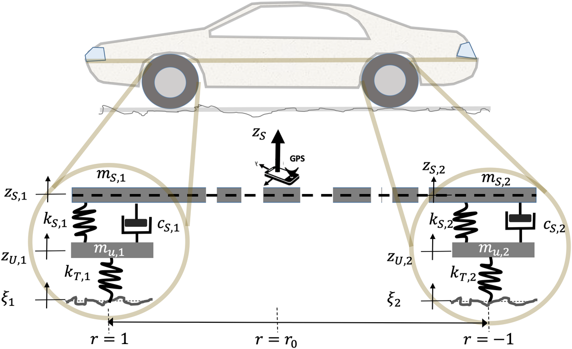
By way of illustration, consider the half-car model $ \left(K=2\right) $ (Figure 1), with interpolation functions defined by:

(12) $$ {N}_1=\frac{1}{2}\left(1+r\right);\quad {N}_2=\frac{1}{2}\left(1-r\right), $$

with $ r=y/\left(L/2\right)\in \left[-1,1\right] $ the dimensionless coordinate along the car axis (i.e., between axles of distance $ L $ ), where $ r=1,\quad -1 $ represent front and back, respectively. In this case, Equation (9) becomes:

(13) $$ {H}_{z_S}(r)=\frac{1}{2}\left(\left(1+r\right)\;{H}_{z_{S,1}}\left(\omega \right)+\left(1-r\right)\quad {H}_{z_{S,2}}\left(\omega \right)\right), $$

where $ {H}_{z_{S,1}} $ and $ {H}_{z_{S,2}} $ are the FRFs of the front and back axles, respectively.

Figure 1.

Schematic of half-car model.

The unknowns of the inverse problem are thus the characteristics of road roughness PSD, $ {S}_{\xi}\left(\omega \right) $ , the vehicle properties of the front- and back-suspension systems, tires (parametrizing the FRFs, $ {H}_{z_S,1} $ and $ {H}_{z_S,2} $ ), and the dimensionless phone position, $ r $ . Their expressions are developed below.

2.2. PSD of road roughness

Road roughness $ \xi $ is a random process over at least two orders of length scales, typically from tens of centimeters to tens of meters. If a flat road is taken as reference, in the first-order approximation, road roughness may be viewed as a zero-mean and stationary white-noise signal. The two first moments (mean and auto-correlation) over some pavement lengths read:

(14) $$ {\left\langle \xi \right\rangle}_L={\mu}_{\xi }=0;\quad {\left\langle \xi (x)\xi \left(x-\lambda \right)\right\rangle}_L={R}_{\xi \xi}\left(\lambda \right)= g\delta \left(\lambda \right), $$

where $ \lambda $ and $ g $ represent the distance lag and the noise strength (of dimension $ \left[g\right]={L}^3 $ ), respectively; the presence of $ \delta \left(\lambda \right) $ function indicates that no correlation exists between any two points on the road profile. The PSD hence reads as:

(15) $$ {S}_0\left(\Omega \right)={\int}_{-\infty}^{\infty }{R}_{\xi \xi}\left(\lambda \right)\exp \left(-i\Omega \lambda \right)\quad \mathrm{d}\lambda =g. $$

For a constant velocity, one can replace distance lag by time lag, $ \lambda =\tau {V}_0 $ , and the angular wave number by the angular frequency $ \omega =\Omega {V}_0 $ . Thus, from Equation (15), the link between $ {S}_0\left(\Omega \right) $ and $ {S}_0\left(\omega \right) $ reads:

(16) $$ {S}_0\left(\Omega \right)={V}_0{S}_0\left(\omega \right)=g. $$

Most spatial representations of the road elevations, however, assume that the white Gaussian noise of strength $ {S}_0\left(\Omega \right)=g $ is filtered by some low-pass filter at the tire–pavement interface (Alessandroni et al., Reference Alessandroni, Carini, Lattanzi, Freschi and Bogliolo2017), with a PSD defined by:

(17) $$ {S}_{\xi}\left(\Omega \right)={S}_0\left(\Omega \right){\left|H\left(\Omega \right)\right|}^2=g\quad {\left|H\left(\Omega \right)\right|}^2, $$

where $ H\left(\Omega \right) $ is the filter’s angular wave number response function (or transfer function). Such a low-pass filter passes signals with an angular wave number $ \Omega $ lower than a selected cutoff wave number $ {\Omega}_0 $ , and attenuates signals with angular wave numbers higher than the cutoff value. For instance, a first-order low-pass filter, for which $ H\left(\Omega \right)={\left(1+i\left(\Omega /{\Omega}_0\right)\right)}^{-1} $ , provides the following road roughness PSD:

(18) $$ {S}_{\xi}\left(\Omega \right)=g{\left|\frac{1}{1+i\left(\Omega /{\Omega}_0\right)}\right|}^2, $$

or in terms of the angular frequency using Equation (16):

(19) $$ {S}_{\xi}\left(\omega \right)=\frac{S_{\xi}\left(\Omega \to \omega /{V}_0\right)}{V_0}=g{\Omega}_0^2{V}_0{\left|\frac{1}{\omega_0+ i\omega}\right|}^2, $$

where $ {\omega}_0={V}_0{\Omega}_0 $ is the cut-off angular frequency. A further refinement of this first-order low-pass filter takes the form of a power-scaling:

(20) $$ {S}_{\xi}\left(\Omega \right)=g{\left|\frac{1}{1+i{\left(\Omega /{\Omega}_0\right)}^{w/2}}\right|}^2\quad \simeq \quad g{\left(\frac{\Omega}{\Omega_0}\right)}^{-w}, $$

or in terms of the angular frequency:

(21) $$ {S}_{\xi}\left(\omega \right)=g{\Omega}_0^w{V}_0^{w-1}{\left|\frac{1}{\omega_0^{w/2}+i{\omega}^{w/2}}\right|}^2\quad \simeq \quad g{\Omega}_0^w{V}_0^{w-1}{\omega}^{-w}, $$

where $ w $ —in pavement engineering—goes by the name of waviness index, and $ g{\Omega}_0^w $ is the unevenness number. The approximations in Equations (20) and (21), which suppress the pole in the filter expressions are at the core of realistic description of road surface roughness in pavement engineering (Dodds and Robson, Reference Dodds and Robson1973; Kropáč and Múčka, Reference Kropáč and Múčka2008).

2.3. FRF: half-car model

Vehicle dynamics models for investigation of ride comfort and overall vehicle performance are abundant in the literature, ranging from quarter-car models to full-car models. Here we focus on the half-car model (Figure 1), which has specific features of interest for analyzing smartphone measurements. More specifically, acceleration measurements of a smartphone in a specific position within a car are affected by both front and back accelerations. A half-car model is thus chosen as it accommodates phone position (Equations 3–7).

2.3.1 Mass distribution model

Classical half-car models are four degree-of-freedom models that employ a longitudinally distributed sprung mass density together with two unsprung masses to describe vehicle dynamics in terms of the movement of the unsprung masses (front and back), the vertical movement of sprung mass’s center of gravity and its pitch angle (i.e., the rotary angle of the vehicle body at the center of gravity) (Gao et al., Reference Gao, Zhang and Du2007). As an alternative, we here suggest the following linear sprung mass distribution:

(22) $$ m(y)={m}_{S,1}{N}_1(y)+{m}_{S,2}{N}_2(y), $$

where $ {m}_{S,1} $ and $ {m}_{S,2} $ are the front and back sprung masses, respectively. The total sprung mass of the vehicle is $ {m}_S={m}_{S,1}+{m}_{S,2} $ . Using the interpolation functions defined by Equation (12), the center of gravity of the sprung mass of the vehicle is (see also Appendix A):

(23) $$ {r}_0=\frac{1}{m_S}{\int}_{-1}^1r\quad m(r)\quad \mathrm{d}r=\frac{1}{3}\frac{m_{S,1}-{m}_{S,2}}{m_{S,1}+{m}_{S,2}}=1-2{\rho}_0, $$

where $ {\rho}_0 $ is the center of gravity measured from the front axle, which relates to the mass moment of inertia of the vehicle, $ {I}_s $ (around the center of gravity) by:

(24) $$ \frac{I_S}{m_S{L}^2}=\frac{1}{8{m}_S}{\int}_{-1}^1m(r){r}^2\mathrm{d}r+{\left({\rho}_0-1/2\right)}^2={\rho}_0^2-{\rho}_0+\frac{7}{24}\ \ge\ \frac{1}{24}. $$

In other words, the mass distribution model accounts for the impact of pitch angle rotation of the vehicle’s inertia. For our purpose, the center of gravity of the vehicle, $ {\rho}_0 $ , is an additional unknown in the inverse analysis.

2.3.2 Equations of motion

The mass distribution model is taken into account in the derivation of the equations of motion of the half-car model using the Lagrangian, that is, $ \mathrm{\mathcal{L}}={E}_k-{E}_p $ where $ {E}_k $ and $ {E}_p $ are the kinetic energy and the potential energy, respectively. The kinetic energy of the half-car model with front and back unsprung masses and sprung mass distribution reads:

(25) $$ {E}_k=\frac{1}{2}{\int}_{-1}^{+1}m(r)\quad {\dot{z}}_S^2(r)\mathrm{d}r+\frac{1}{2}\left({m}_{U,1}{\dot{z}}_{U,1}^2+{m}_{U,2}{\dot{z}}_{U,2}^2\right)=\frac{1}{6}{m}_S\left(\frac{1}{2}{\dot{z}}_{S,1}^2\left(1+2\frac{m_{S,1}}{m_S}\right)+{\dot{z}}_{S,1}{\dot{z}}_{S,2}+\frac{1}{2}{\dot{z}}_{S,2}^2\left(1+2\frac{m_{S,2}}{m_S}\right)\right)\quad +\frac{1}{2}\left({m}_{U,1}{\dot{z}}_{U,1}^2+{m}_{U,2}{\dot{z}}_{U,2}^2\right), $$

where we used expressions (1) and (22). Similarly, the potential energy of the half-car model with front and back suspension systems reads:

(26) $$ {E}_p=\frac{1}{2}{k}_{S,1}{\left({z}_{S,1}-{z}_{U,1}\right)}^2+\frac{1}{2}{k}_{S,2}{\left({z}_{S,2}-{z}_{U,2}\right)}^2+\frac{1}{2}{k}_{T,1}{\left({z}_{U,1}-\xi \right)}^2+\frac{1}{2}{k}_{T,2}{\left({z}_{U,1}-\xi \right)}^2+{F}_{V,1}\left({z}_{S,1}-{z}_{U,1}\right)+{F}_{V,2}\left({z}_{S,2}-{z}_{U,2}\right), $$

where $ \left({k}_{S,1},\quad {k}_{T,1}\right) $ and $ \left({k}_{S,2},\quad {k}_{T,2}\right) $ are the front and back sprung and unsprung stiffness constants, respectively; $ {F}_{V,1} $ and $ {F}_{V,2} $ are the viscous forces in the suspension system. Owing to their non-conservative nature, the viscous forces are considered external work in the expression of the Lagrangian. This choice permits remaining in the classical framework of generalized coordinates underlying Lagrangian mechanics. Therefore, four Euler–Lagrange equations for the four degrees of freedom, $ \mathbf{z}={\left({z}_{S,1},\quad {z}_{U,1},\quad {z}_{S,2},\quad {z}_{U,2}\right)}^T $ provide the set of equations of motion:

(27) $$ \frac{\partial L}{\partial \mathbf{z}}-\frac{\partial }{\partial t}\frac{\partial L}{\partial \mathbf{z}}=0, $$

which in matrix form reads:

(28) $$ \mathbf{M}\cdot \mathbf{z}+\mathbf{C}\cdot \mathbf{z}+\mathbf{K}\cdot \mathbf{z}=\mathbf{F}. $$

• • $ \mathbf{M} $ is the mass matrix:

(29) $$ \mathbf{M}=\frac{m_S}{2}\left[\begin{array}{cccc}\frac{1}{3}\left(1+{\overline{m}}_{S,1}\right)& 0& \frac{1}{3}& 0\\ {}0& {\overline{m}}_1& 0& 0\\ {}\frac{1}{3}& 0& \frac{1}{3}\left(1+{\overline{m}}_{S,2}\right)& 0\\ {}0& 0& 0& {\overline{m}}_2\end{array}\right], $$

with the mass invariants defined by:

(30) $$ {\overline{m}}_1=\frac{m_{U,1}}{m_S/2};\quad {\overline{m}}_2=\frac{m_{U,2}}{m_S/2};\quad {\overline{m}}_{S,1}=\frac{m_{S,1}}{m_S/2};\quad {\overline{m}}_{S,2}=\frac{m_{S,2}}{m_S/2}. $$

• • $ \mathbf{K} $ is the stiffness matrix:

(31) $$ \mathbf{K}={k}_{S,1}\left[\begin{array}{cccc}1& -1& 0& 0\\ {}-1& 1+{\overline{k}}_1& 0& 0\\ {}0& 0& \kappa & -\kappa \\ {}0& 0& -\kappa & \kappa \left(1+{\overline{k}}_2\right)\end{array}\right], $$

where the stiffness invariants read:

(32) $$ {\overline{k}}_1=\frac{k_{T,1}}{k_{S,1}};\quad \kappa =\frac{k_{S,2}}{k_{S,1}};\quad {\overline{k}}_2=\frac{k_{T,2}}{k_{S,2}}. $$

• • $ \mathbf{C} $ is the damping matrix, which is obtained considering the viscous suspension forces, $ {F}_{V,i}={c}_{S,i}\left({\dot{z}}_{S,i}-{\dot{z}}_{U,i}\right) $ , where $ {c}_{S,i} $ is the damping coefficient:

(33) $$ \mathbf{C}={c}_{S,1}\left[\begin{array}{cccc}1& -1& 0& 0\\ {}-1& 1& 0& 0\\ {}0& 0& \gamma & -\gamma \\ {}0& 0& -\gamma & \gamma \end{array}\right], $$

with the damping invariants of the half-car model defined by:

(34) $$ \gamma =\frac{c_{S,2}}{c_{S,1}};\quad \zeta =\frac{c_{S,1}}{2\sqrt{\left({m}_S/2\right){k}_{S,1}}}={\zeta}_1\sqrt{{\overline{m}}_{S,1}}=\frac{\sqrt{{\overline{m}}_{S,2}\kappa }}{\gamma }{\zeta}_2, $$

where $ {\zeta}_i={c}_{S,i}/2\sqrt{m_{S,i}{k}_{S,i}} $ are front $ \left(i=1\right) $ and back $ \left(i=2\right) $ damping ratios.

• • $ \mathbf{F} $ is the force vector due to road roughness excitation:

(35) $$ \mathbf{F}=\xi {k}_{S,1}{\left(0,{\overline{k}}_1,0,{\overline{k}}_2\kappa \right)}^T. $$

2.3.3 Frequency response function

The FRF is defined, in Fourier domain, as the linear operator that maps the excitation, $ \hat{\xi} $ , to the displacement, that is,

(36) $$ \hat{\mathbf{z}}={\mathbf{H}}_{\mathbf{z}}\hat{\xi};\quad {\mathbf{H}}_{\mathbf{z}}={\left({H}_{z_{S,1}},{H}_{z_{U,1}},{H}_{z_{S,2}},{H}_{z_{U,2}}\right)}^T. $$

The FRF is thus obtained from the Fourier transform of the equations of motion:

(37) $$ \hat{\mathbf{K}}\cdot \hat{\mathbf{z}}=\left(-{\omega}^2\mathbf{M}+ i\omega \mathbf{C}+\mathbf{K}\right)\cdot \hat{\mathbf{z}}=\hat{\mathbf{F}}. $$

That is, letting Equation (36) in (37):

(38) $$ {\mathbf{H}}_{\mathbf{z}}=\frac{1}{\hat{\xi}}{\hat{\mathbf{K}}}^{-1}\cdot \hat{\mathbf{F}}. $$

For the half-car model, we have:

(39) $$ \hat{\mathbf{K}}={k}_{S,1}\left[\begin{array}{cccc}1-{\overline{\omega}}^2\frac{1}{3}\left(1+{\overline{m}}_{S,1}\right)+2i\overline{\omega}\zeta & -\left(1+2i\overline{\omega}\zeta \right)& -\frac{1}{3}{\overline{\omega}}^2& 0\\ {}-\left(1+2i\overline{\omega}\zeta \right)& 1+{\overline{k}}_1-{\overline{\omega}}^2{\overline{m}}_1+2i\overline{\omega}\zeta & 0& 0\\ {}-\frac{1}{3}{\overline{\omega}}^2& 0& \kappa -{\overline{\omega}}^2\frac{1}{3}\left(1+{\overline{m}}_{S,2}\right)+2i\overline{\omega}\zeta \gamma & -\left(\kappa +2i\overline{\omega}\zeta \gamma \right)\\ {}0& 0& -\left(\kappa +2i\overline{\omega}\zeta \gamma \right)& \kappa \left(1+{\overline{k}}_2\right)-{\overline{\omega}}^2{\overline{m}}_2+2i\overline{\omega}\zeta \gamma \end{array}\right], $$

and

(40) $$ \hat{\mathbf{F}}={k}_{S,1}\hat{\xi}{\left(0,{\overline{k}}_1,0,\kappa {\overline{k}}_2\right)}^T, $$

where $ \overline{\omega}=\omega /{\omega}_S $ is the angular frequency normalized by $ {\omega}_S=\sqrt{k_{S,1}/\left({m}_S/2\right)} $ , which relates to front ( $ {\omega}_{S,1} $ ) and back $ \left({\omega}_{S,2}\right) $ frequency of the suspension system by:

(41) $$ {\omega}_S^2=\frac{k_{S,1}}{m_S/2}={\overline{m}}_{S,1};\quad {\omega}_{S,1}^2=\frac{{\overline{m}}_{S,1}}{\kappa }{\omega}_{S,2}^2;\quad {\omega}_{S,i}^2=\frac{k_{S,i}}{m_{S,i}}. $$

3.1. Unknowns

The inverse analysis infers the following 13 unknowns from acceleration measurements of a smartphone, and vehicle speed determined from GPS measurements:

(42) $$ \theta =\left(g{\Omega}_0^w,\quad w,\quad {f}_S,\quad {\overline{k}}_1,\quad {\overline{k}}_2,\quad \kappa, \quad {\overline{m}}_1,\quad {\overline{m}}_2,\quad {\overline{m}}_{S,1},\quad {\overline{m}}_{S,2},\quad {\zeta}_1,\quad {\zeta}_2,\quad {r}_p\right). $$

Namely:

1. 1. Two road roughness PSD parameters of $ {S}_{\xi}\left(\Omega \right) $ ; for instance, from Equation (20), the unevenness index ( $ g{\Omega}_0^w $ ) and the waviness number ( $ w $ ). These two parameters permit the determination of road roughness quantifiers, such as the IRI. As a reminder, IRI is defined as the accumulated suspension motion of the GC traveling at a fixed reference speed ( $ {V}_{REF}=80\quad \mathrm{km}/\mathrm{h} $ ) over a distance ( $ {L}_{REF} $ ), which reads (Sayers, Reference Sayers1995; Sayers and Karamihas, Reference Sayers and Karamihas1998; Louhghalam et al., Reference Louhghalam, Tootkaboni and Ulm2015):

(43) $$ \mathrm{IRI}=\frac{1}{V_{REF}}\unicode{x1D53C}{\left[{\left|\dot{z}\right|}_{\mathrm{GC}}\right]}_{L_{REF}}=\chi \sqrt{\int_0^{\infty }{\Omega}^2{\left|{H}_z^{\mathrm{GC}}\right|}^2\quad {S}_{\xi}\left(\Omega \right)\quad \mathrm{d}\Omega}, $$

where $ {H}_z^{\mathrm{GC}} $ is the FRF of the GC model of known properties; $ \chi =\unicode{x1D53C}{\left[{\left|\dot{z}\right|}_{\mathrm{GC}}\right]}_{L_{REF}}/\sqrt{\unicode{x1D53C}{\left[{\dot{z}}_{\mathrm{GC}}^2\right]}_{L_{REF}}} $ is a constant relating the mean-square of the zero-mean random process $ \dot{z} $ to the expected value of its absolute value. A Gaussian roughness profile, for instance, results in a normally distributed suspension motion with $ \chi =\sqrt{2/\pi } $ (for other marginal probability distributions; see Louhghalam et al., Reference Louhghalam, Tootkaboni and Ulm2015). A convenient asymptotic solution for Equation (43) has recently been proposed in the function of only the road roughness PSD parameters, $ \left(g{\Omega}_0^w\right) $ and $ w $ (Louhghalam et al., Reference Louhghalam, Tootkaboni, Igusa and Ulm2019):

(44) $$ \mathrm{IRI}=\sqrt{\frac{\left(g{\Omega}_0^w\right)}{2{\zeta}^{\mathrm{GC}}}{\left(\frac{\omega_S^{\mathrm{GC}}}{V_{REF}}\right)}^{3-w}\left(1+{\left(\frac{{\overline{k}}^{\mathrm{GC}}}{{\overline{m}}^{\mathrm{GC}}}\right)}^{1-w/2}\left({\overline{k}}^{\mathrm{GC}}-\frac{w}{2}\right)\right)}, $$

where $ 2{\zeta}^{\mathrm{GC}}={c}_S^{\mathrm{GC}}/\sqrt{k_S^{\mathrm{GC}}{m}_S^{\mathrm{GC}}}=0.75 $ ; $ {\omega}_S^{\mathrm{GC}}=\sqrt{k_S^{\mathrm{GC}}/{m}_S^{\mathrm{GC}}}=8.0\quad \mathrm{rad}/\mathrm{s} $ ; $ {\overline{k}}^{\mathrm{GC}}={k}_T^{\mathrm{GC}}/{k}_S^{\mathrm{GC}}=10.3;{\overline{m}}^{\mathrm{GC}}={m}_T^{\mathrm{GC}}/{m}_S^{\mathrm{GC}}=0.15 $ are known parameters of the GC model (Sayers, Reference Sayers1995; Sayers and Karamihas, Reference Sayers and Karamihas1998).

1. 2. The vehicle properties of the half-car model; that is, according to Equations (39)–(41).

• • The fundamental frequency of the suspension system, $ {f}_S $ , from which the front and rear suspension systems can be derived (Equation (41)).

• • Three stiffness invariants: the front and rear stiffness ratios, $ {\overline{k}}_i $ , and the rear-to-front suspension spring stiffness ratio, $ \kappa $ (Equation (32)).

• • Four mass invariants: the front and rear unsprung-to-sprung half mass ratio, $ {\overline{m}}_i $ , and the front and rear sprung mass loading factors, $ {\overline{m}}_{S,i} $ , which define the sprung mass’s moment of inertia and center of gravity (Equations (23), (24), and (30)).

• • Two damping ratios: the front and rear damping ratios, $ {\zeta}_i $ (Equation (34)).

1. 3. The phone position along the vehicle axis, $ {r}_p $ , which is used to interpolate the front and rear FRF (Equation (13)).

3.2. From acceleration measurements to acceleration PSD

The input of the inverse analysis is the time series of vertical acceleration measurements of a smartphone. Since smartphones measure accelerations in three orthogonal directions of a local phone-specific coordinate system (Figure 2), these measurements need to be orthogonally projected to the road surface. This is readily achieved by means of the angles measured by the phone’s gyroscope sensors, which link the phone’s local coordinate system to a North–East–Gravity (NEG) coordinate system; that is:

(45) $$ {a}_z\left({r}_p\right)={\overrightarrow{e}}_z\cdot \overrightarrow{a}\left({r}_p\right)=-{a}_X\sin \theta \quad +{a}_Y\left(\sin \phi \cos \theta \right)+{a}_Z\left(\cos \phi \cos \theta \right), $$

where $ {\overrightarrow{e}}_z $ is the gravity direction, $ \overrightarrow{a}\left({r}_p\right)=\left({a}_X,{a}_Y,{a}_Z\right) $ denotes the accelerations measured in the phone’s local coordinate system $ \left({\overrightarrow{e}}_X,{\overrightarrow{e}}_Y,{\overrightarrow{e}}_Z\right) $ , and $ \left(\phi, \theta \right) $ are the Euler angles measured by the phone’s gyroscope which define the position of the phone w.r.t. the NEG—system of coordinates.

Figure 2.

Local right-handed phone-specific coordinate system (adapted from Keller, Reference Keller2015).

Smartphone acceleration measurements are carried out with a sampling frequency of $ {F}_s=100\quad \mathrm{Hz} $ . The analysis is then performed with a moving time window, $ {\tau}_W $ . This time window must be sufficiently large so as to ensure the stationarity condition required to employ the underlying assumption of the PSD-analysis, namely the Wiener–Khintchine theorem (Khintchine, Reference Khintchine1934; Champeney, Reference Champeney1987). Thus, corrected for the mean value, the input signal for the PSD-analysis is $ {\ddot{z}}_S(t)={a}_z\left({r}_p,t\right)-\unicode{x1D53C}{\left[{a}_z\left({r}_p,t\right)\right]}_{\tau_W} $ , which passes classical time-series stationarity or trend-stationarity tests (e.g., the Augmented Dickey–Fuller test), with a mean value close to the earth acceleration $ g=9.8\quad \mathrm{m}/{\mathrm{s}}^2 $ , that is, $ |\unicode{x1D53C}{\left[{a}_z\left({r}_p,t\right)\right]}_{\tau_W}|=g\left(1+\varepsilon \right) $ with $ \left|\varepsilon \right| \ll 1 $ .

With a focus on estimating PSD of road roughness and to minimize the effects of speed variations within the time window, the determination of acceleration PSD converts the signal from the length domain to the angular wave number domain by considering the angular wave number $ {\Omega}_s=2\pi {F}_s/{V}_0 $ , where $ {V}_0=\unicode{x1D53C}{\left[V(t)\right]}_{\tau_W} $ is the mean speed in the time window for sampling frequency. This readily achieved by employing classical tools of signal processing such as the Welch method for spectral density estimation. The resulting experimental input for the inverse analysis is thus $ {S}_{{\ddot{z}}_S}^{\mathrm{exp}}\left(\Omega \right)={V}_0{S}_{{\ddot{z}}_S}^{\mathrm{exp}}\left(\omega \right) $ .

3.3. Parameter identification

The parameter identification then considers the error between the experimental acceleration PSD, $ {S}_{{\ddot{z}}_S}^{\mathrm{exp}}\left(\omega =\Omega {V}_0\right) $ , and the half-car model PSD, as defined by Equations 3, 8, 13, 21, and 38, which reads:

(46) $$ {S}_{{\ddot{z}}_S}^{\mathrm{mod}}\left(\omega \right)={\omega}^4{\left|{H}_{z_S}\left({r}_p,\omega \right)\right|}^2{S}_{\xi}\left(\omega \right). $$

That is, in a logarithmic base:

(47) $$ \log ({S}_{{\ddot{z}}_S}^{\mathrm{mod}}\left(\omega \right))=4\log \left(\omega \right)+2\log \left(\left|{H}_{z_S}\left({r}_p,\omega \right)\right|\right)+\log {S}_{\xi}\left(\omega \right). $$

One can thus define the root mean square error, $ {\left|\left|{\Delta}_{{\ddot{z}}_S}\left(\omega \right)\right|\right|}_2 $ , which explicitly accounts for the unknown PSD parameters of road roughness (Equation (21)) ( $ g{\Omega}_0^w $ and $ w $ ; see Appendix A), from the logarithmic difference between experimental and model acceleration PSD as:

(48) $$ {\Delta}_{{\ddot{z}}_S}\left(\omega \right)=\log {S}_{{\ddot{z}}_S}^{\mathrm{exp}}\left(\omega \right)-\log {S}_{{\ddot{z}}_S}^{\mathrm{mod}}\left(\omega \right)=\log {S}_{{\ddot{z}}_S}^{\mathrm{exp}}\left(\omega \right)-\left(4-w\right)\log \left(\omega \right)-2\log \left(\left|{H}_{z_S}\left({r}_p,\omega \right)\right|\right)-\log \left(g{\Omega}_0^w\right)+\left(1-w\right)\log {V}_0. $$

Hence, as $ {\left|\left|{\Delta}_{{\ddot{z}}_S}\right|\right|}_2\ \to\ 0 $ , $ \exp \left({\left|\left|{\Delta}_{{\ddot{z}}_S}\right|\right|}_2\right)\quad \to \quad 1 $ , and $ {S}_{{\ddot{z}}_S}^{\mathrm{exp}}/{S}_{{\ddot{z}}_S}^{\mathrm{mod}}\ \to 1 $ . The minimization problem, however, is ill-posed as it admits a large number of possible solutions due to its additive structure (Equation (48)). Additional constraints are thus required to restore well-posedness; for instance, regularizing the minimization problem by a smooth term such as owing to its convexity, the L2 norm of the difference between the model parameters and a set of reference values $ {\theta}_{i, ref} $ via:

(49) $$ \underset{\theta }{\min}\left(\exp {\left|\left|{\Delta}_{{\ddot{z}}_S}\left(\theta \right)\right|\right|}_2-1\right)\left(1+\alpha \sum \limits_{\theta_i\in {\Theta}_c}{\left(\frac{\theta_i}{\theta_{i, ref}}-1\right)}^2\right), $$

with $ \alpha $ denoting car regularization parameter; $ {\Theta}_c $ represents a subset of half-car parameters which contributes to restoring the well-posedness of the minimization problem while ensuring the transferability of the approach from one vehicle type to another. Furthermore, the regularization function does not include road roughness metrics to refrain any constraint on road roughness metrics, thus securing transferability w.r.t. road class. The regularization term in Equation (49) can be enhanced by elements of statistical learning to update the reference values $ {\theta}_{i, ref} $ in a continuous time series analysis (e.g., see Evgeniou et al., Reference Evgeniou, Poggio, Pontil and Verri2002).

3.4. Energy dissipation

The mechanistic-based inverse analysis thus provides the means to determine road roughness parameters, vehicle properties, and phone position from the measured acceleration time series in each time window. These quantities are key to derive important additional information such as the energy dissipated in the (model) vehicle’s suspension system. Evoking the fluctuation–dissipation theorem (Kubo, Reference Kubo1966), the energy dissipated in the suspension system per distance driven is:

(50) $$ \delta {E}_i=\frac{c_i}{V_0}\unicode{x1D53C}\left[{\dot{z}}_i^2\right], $$

where the mean square of suspension motion $ \unicode{x1D53C}\left[{\dot{z}}_i^2\right] $ is obtained from the suspension motion PSD, $ {S}_{\dot{z}}\left(\omega \right) $ , in the form (Louhghalam et al., Reference Louhghalam, Tootkaboni and Ulm2015):

(51) $$ \unicode{x1D53C}\left[{\dot{z}}_i^2\right]={\int}_0^{\infty }{S}_{\dot{z}}\left(\omega \right)\quad \mathrm{d}\omega ={\int}_0^{\infty }{\omega}^2{\left|{H}_{z_{S,i}}-{H}_{z_{U,i}}\right|}^2{S}_{\xi}\left(\omega \right)\quad \mathrm{d}\omega, $$

where $ {H}_{z_{S,i}} $ and $ {H}_{z_{U,i}} $ respectively denote the sprung mass and unsprung mass FRFs of the front $ \left(i=1\right) $ and rear $ (i=2) $ suspension system, that is, from the solution of Equation (36). Since the integral expression in Equation (51) converges rapidly, an estimate of the energy dissipated in the suspension system can be obtained from an asymptotic solution of Equation (50) for the quarter-car model (Louhghalam et al., Reference Louhghalam, Tootkaboni, Igusa and Ulm2019). Using the model invariants (30) and (32), this asymptotic model holds—in first order—for the front and rear suspension system as:

(52) $$ {\Pi}_i=\frac{\delta {E}_i}{\left(g{\Omega}_0^w\right){V}_0^{w-2}{m}_{S,i}\quad {\omega}_{S,i}^{4-w}}=\frac{\pi }{2}\left(1+{\left(\frac{{\overline{k}}_i}{{\overline{m}}_i{\overline{m}}_{S,i}}\right)}^{1-w/2}\left({\overline{k}}_i-\frac{w}{2}\right)\right). $$

Whence the specific energy dissipation of the half-car model (of dimension $ \left[\mathrm{Energy}\right] $ M $ {}^{-1} $ L $ {}^{-1}= $ LT $ {}^{-2} $ ):

(53) $$ {E}_d=\frac{\delta {E}_1+\delta {E}_2}{m_S}=\left(g{\Omega}_0^w\right){V}_0^{w-2}{\omega}_S^{4-w}{\overline{m}}_{S,1}^{w/2-1}\frac{1}{2}\left({\Pi}_1+{\kappa}^{2-w/2}\frac{{\overline{m}}_{S,2}}{{\overline{m}}_{S,1}}{\Pi}_2\right). $$

The specific energy dissipation is an interesting synergistic cost quantity combining vehicle properties ( $ {f}_S,\quad {\overline{k}}_i,\quad \kappa, \quad {\overline{m}}_i,\quad {\overline{m}}_{S,i} $ ), road roughness parameters ( $ g{\Omega}_0^w,\quad w $ ), and vehicle operational conditions (speed $ {V}_0 $ ). This shows the relevance of the proposed inverse approach for crowdsourced road roughness-induced vehicle energy consumption.

4.1. Experimental data set

Laser measurements of road roughness profiles were acquired by a commercially available service which employs a state-of-the-art multifunction vehicle for conducting pavement profile and surface condition assessment (Dynatest, 2019). The vehicle was equipped with a road surface profiler (Dynatest Road Surface Profiler Model 5051 Mark III), five laser sensors and two accelerometers to cover up to 3.6 m width of traveled lane, and an inertial profiler system and 3D laser crack measurement system which permits collecting pavement longitudinal and transverse profile and surface condition data in one pass. Data collection was performed under prevailing traffic conditions (no hindrance to traffic) during daytime and dry weather conditions. Two test tracks were investigated (Figure 3a): (a) 13.8 km centerline miles on two lanes of a thoroughfare with a dominating inner-city component, and (b) 11.6 km centerline miles of a highway on three lanes, thus a total of 62.4 km.

Figure 3.

Direct measurements of road roughness from laser measurements for the two test tracks: (a) Coordinates of the test tacks. (b) PDF of road roughness for the experiments and their corresponding zero-mean Gaussian fit in dashed lines. Laser-measured longitudinal profiles of (c) test track 1 and (d) test track 2.

4.1.1 Longitudinal profile measurements (direct measurements)

The laser-measured longitudinal profile for the two test tracks are illustrated in Figure 3 in form of an elevation plot, together with a probability density function (PDF) of the elevation in Figure 3b. Of particular interest for the pursuing analysis are the following observations:

1. 1. The elevation PDFs exhibit symmetry (zero skewness) and zero mean (Figure 3b). This, in turn, implies that forces generated by this road roughness can be viewed as a symmetric zero-mean stationary process, which is the underlying assumption of our PSD-modeling approach.

2. 2. The elevation fluctuations of the two test tracks are substantially different. Precisely, elevation fluctuations of the inner-city test track 1 are approximately three times the values of the highway test track 2, that is, $ {\sigma}_{\xi}^{(1)}/{\sigma}_{\xi}^{(2)} \approx 3 $ where $ {\sigma}_{\xi }=\sqrt{{\left\langle {\left(\xi -{\left\langle \xi \right\rangle}_L\right)}^2\right\rangle}_L} $ is the elevation standard deviation with $ <.> $ representing the average (mean) operator. This suggests that the road roughness noise strength $ g $ (Equations (14) and (15)) between the two test roads exhibit an overall ratio of $ {g}^{(1)}/{g}^{(2)}\simeq \quad 9 $ . The average IRI should hence scale, on average, as $ \Big\langle $ IRI $ \left\rangle {}_L^{(1)}/\right\langle $ IRI $ \Big\rangle {}_L^{(2)} \simeq {\sigma}_{\xi}^{(1)}/{\sigma}_{\xi}^{(2)} \approx 3 $ , provided similar value distributions of the road roughness waviness number $ w $ (Equation (44)).

We proceed by analyzing the spatially varying roughness PSD of the measurements. This is achieved by considering a length window of 800 m moving with a constant distance of 50 m over the elevation data of the two test tracks. The model PSD, $ {S}_{\xi}\left(\Omega \right)\quad \simeq g{\left(\Omega /{\Omega}_0\right)}^{-w} $ (Equation (20)), is fitted to the experimental PSD for each window to obtain the spatial variation of roughness metrics as shown in Figure 4a,b. The statistics of such roughness metrics (Figure 4c,d) confirm that, in a global sense, both unevenness index and waviness number show higher values in the rougher road. More precisely, the mean ratios for waviness number and unevenness index of the two tracks read as $ {\left\langle w\right\rangle}_L^{(1)}/{\left\langle w\right\rangle}_L^{(2)}\quad \approx \quad 1.3 $ and $ {\left\langle g{\Omega}_0^w\right\rangle}_L^{(1)}/{\left\langle g{\Omega}_0^w\right\rangle}_L^{(2)}\quad \approx \quad 2.1 $ . The mean value of IRI is then obtained via Equation (44) at the mean points, thus leading to $ \Big\langle $ IRI $ \left\rangle {}_L^{(1)}/\right\langle $ IRI $ \Big\rangle {}_L^{(2)}\quad \simeq \quad 3.5 $ . Furthermore, the standard deviation of IRI can be calculated from that of waviness number and unevenness index using the multivariate delta method given by,

(54) $$ {\sigma}_{\mathrm{IRI}} \approx \sqrt{u^t\cdot \mathbf{V}\cdot u}, $$

where $ u $ is the gradient of IRI (i.e., $ u=\nabla \mathrm{IRI}={\left(\mathrm{\partial IRI}/\partial \left(g{\Omega}_0^w\right),\mathrm{\partial IRI}/\partial w\right)}^T $ ) and $ \mathbf{V} $ is the covariance matrix:

(55) $$ \mathbf{V}=\left[\begin{array}{cc}{\left({\sigma}_{g{\Omega}_0^w}\right)}^2& {\sigma}_{w,g{\Omega}_0^w}\\ {}{\sigma}_{w,g{\Omega}_0^w}& {\left({\sigma}_w\right)}^2\end{array}\right], $$

The off-diagonal elements of $ \mathbf{V} $ are almost zero, implying that $ w $ and $ g{\Omega}_0^w $ are truly two uncorrelated quantities characterizing road roughness PSD. The ratios of standard deviation for the PSD-inferred roughness metrics are $ {\sigma}_w^{(1)}/{\sigma}_w^{(2)}\quad \approx \quad 0.5 $ and $ {\sigma}_{g{\Omega}_0^w}^{(1)}/{\sigma}_{g{\Omega}_0^w}^{(2)} \approx \quad 1.9 $ for waviness number and unevenness index, respectively. Substituting the statistical moments of $ g{\Omega}_0^w $ and $ w $ in Equation (54) yields $ {\sigma}_{\mathrm{IRI}}^{(1)}/{\sigma}_{\mathrm{IRI}}^{(2)} \approx \quad 2.7 $ , which confirms that inner-city IRI values exhibit larger fluctuations compared to the highway.

Figure 4.

Spatial variation of roughness metrics inferred from measured roughness PSD: unevenness index $ g{\Omega}_0^w $ and waviness number $ w $ for (a) test track 1 and (b) test track 2. Distribution of (c) waviness number and (d) unevenness index for the two test tracks.

4.1.2 Derived roughness metrics: IRI

We remind ourselves that IRI is not a direct measurable quantity but a derived quantity representing the length-averaged motion of the suspension system of the GC traveling at a constant reference speed of $ {V}_{REF}=80\quad \mathrm{km}/\mathrm{h} $ ; that is (Sayers, Reference Sayers1995; Sayers and Karamihas, Reference Sayers and Karamihas1998):

(56) $$ \mathrm{IRI}=\frac{1}{L_w}{\int}_0^{\tau_w}\left|{\dot{z}}_{\mathrm{GC}}\right|\quad \mathrm{d}t, $$

where $ {L}_w={V}_{REF}{\tau}_w $ is the segment length (corresponding here to the length window), $ {\tau}_w $ the residence time in the segment length when the vehicle moves at the reference speed; $ {z}_{\mathrm{GC}} $ is the suspension motion of the GC subject to dynamic excitation of the road profile. There are two ways of determining the IRI from elevation measurements, namely direct time-domain integration of the equations of motion of the quarter car model (ProVAL, 2017), or inverse Fourier transform using the FRF $ {H}_z^{\mathrm{GC}}\left(\omega \right) $ of the GC (i.e., $ {\dot{z}}_{\mathrm{GC}}={\int}_{-\infty}^{+\infty } i\omega {H}_z^{\mathrm{GC}}\left(\omega \right){\hat{\xi}}_t\left(\omega \right)\quad \mathrm{d}\omega $ , with $ {\hat{\xi}}_t\left(\omega \right) $ the Fourier transform of the temporal excitation of the spatial roughness profile transformed via the time–space correspondence $ x={V}_{REF}\quad t $ ). The time-domain integration includes both transient and steady-state responses. The transient part, however, decays exponentially in strongly damped systems such as the GC model, converging quickly to the steady-state solution captured by the inverse Fourier transform approach (Botshekan et al., Reference Botshekan, Tootkaboni and Louhghalam2019). Otherwise said, a large enough length window, $ {L}_w $ , ensures the compatibility of time and frequency approaches in determining IRI.

Based on this compatibility, we can further compare direct determination methods of IRI with the indirect method stipulated in our model using random vibration theory, as exemplified by Equation (43) and its asymptotic form in Equation (44). Specifically, in contrast to the direct methods (whether in time or frequency domain), the random-vibration-theory-based approach requires the stochastic nature of the suspension motion in form of a multiplying constant, $ \chi =\unicode{x1D53C}{\left[{\left|\dot{z}\right|}_{\mathrm{GC}}\right]}_{L_w}/\sqrt{\unicode{x1D53C}{\left[{\dot{z}}_{\mathrm{GC}}^2\right]}_{L_w}} $ (Equation (43)), as input. Figure 5 displays the probability distribution of $ \chi $ obtained for the two test tracks. A peak close to $ {\chi}_G=\sqrt{2/\pi } $ is found which implies that the distribution of the suspension motion is predominantly Gaussian (Louhghalam et al., Reference Louhghalam, Tootkaboni and Ulm2015). This suggests that road roughness, on the $ {L}_w $ -length scale, is expected to be normally distributed for the two test tracks. It should, however, be noted that the lower-fluctuation test track 2 shows a secondary peak around $ \chi /{\chi}_G\quad \approx \quad 0.75 $ . This suggests that, while road roughness, as a random process, in test track 2 is predominantly Gaussian, there is a secondary dominant distribution that roughly resembles Laplace distribution with $ {\chi}_L/{\chi}_G\quad \approx 0.85 $ (Louhghalam et al., Reference Louhghalam, Tootkaboni and Ulm2015). Further evidence for the Gaussian nature of roughness distribution is depicted in the inset of Figure 5 which dispalys the probability distribution of higher-order central moments for road roughness, namely skewness ( $ 3\mathrm{rd} $ order) and excess kurtosis ( $ 4\mathrm{th} $ order), exhibiting a maximum around zero.

Figure 5.

Distribution of $ \chi $ exhibiting a peak around $ {\chi}_G=\sqrt{2/\pi } $ . The inset shows the skewness (dashed line) and the excess kurtosis (solid line) of road roughness.

In what follows, for the pursuing calibration and validation of roughness metrics derived from smartphone acceleration measurements, we consider the direct time-integrated IRI measurement as reference, which will be labeled $ {\mathrm{IRI}}^{\mathrm{exp}} $ . The $ {\mathrm{IRI}}^{\mathrm{exp}} $ values for the two test tracks are shown in Figure 6a,c, with the inner-city thoroughfare (test track 1) exhibiting, on average, three times higher IRI than the outer-city highway. In addition, as shown by the difference in standard deviations, stronger fluctuations of IRI around the mean value for the rougher road are clear in Figure 6a,c.

Figure 6.

Calibration-validation results: experimental and model IRI ( $ L=800\quad \mathrm{m} $ , $ {\tau}_W=45\quad \mathrm{s} $ ) for (a) test track 1 and (c) test track 2. Distribution of absolute relative error to quantify the accuracy of the proposed inverse method for (b) tracks 1 and (d) test track 2.

4.2. Calibration—validation of smartphone enabled roughness measurements

The inverse approach developed in this paper employs an L2 norm regularization to estimate the IRI from the acceleration PSD. This regularization involves a set of reference values, $ {\theta}_{i, ref} $ (Equation (49)) for the unknowns of the problem (Equation (42)). Overall validation of smartphone-enabled roughness identification is achieved through a two-step calibration-validation procedure, in which one part of the acquired data is used for calibration, and the other part for validation. With a focus on transferability of the calibrated reference values, we consider the high-fluctuation inner-city thoroughfare (test track 1) for calibration, and the low fluctuation highway data set (test track 2) for validation.

4.2.1 Calibration

The experimental set-up for calibration comprises a vehicle with three smartphones (“sensors”) placed at different locations of the vehicle, namely a phone holder attached to the bottom left of the front windshield (Figure 7a), a cup holder in between the front seats (Figure 7b), and a fixture on the floor behind the right passenger seat (Figure 7c). The outputs of each sensor are the acceleration signal recorded at a 100 Hz frequency, the vehicle speed obtained from vehicle’s GPS coordinates recorded at a 1 Hz frequency (Figure 8). The inverse analysis proceeds by considering a $ {\tau}_w=45 $ s time window moving forward with a time distance of $ \Delta {\tau}_w=1\quad \mathrm{s} $ . For each time window, the inverse approach provides values for the unknowns: road roughness parameters ( $ g{\Omega}_0^w,\quad w $ ) or equivalently ( $ \mathrm{IRI},\quad w $ ), vehicle properties ( $ {f}_S,\quad {\overline{k}}_1,\quad {\overline{k}}_2,\quad {\overline{m}}_1,\quad {\overline{m}}_2,\quad \rho, \quad {\zeta}_1,\quad {\zeta}_2,\quad \kappa $ ), and phone position $ {r}_p $ . The calibration of the L2 norm reference values, $ {\theta}_{i, ref} $ , is achieved by simultaneously minimizing (a) the L2-norm regularized form of the PSD fit for each time window (Equation (49)) and (b) the overall difference between measured and derived IRI values for the entire test track; that is:

(57) $$ \underset{\theta_{i, ref}}{\min}\sum \limits_{(j)}\delta {\mathrm{\mathcal{E}}}_j^2;\quad \delta {\mathrm{\mathcal{E}}}_j=1-\frac{{\mathrm{IRI}}^{\mathrm{mod}}\left({x}_j\right)}{{\mathrm{IRI}}^{\mathrm{exp}}\left({x}_j\right)} $$

where $ {\mathrm{IRI}}^{\mathrm{mod}}\left({x}_j\right) $ is the model IRI-value for time window $ j $ centered at mid-segment position $ {x}_j $ obtained from the fitted model parameters, $ g{\Omega}_0^w\left({x}_j\right) $ and $ w\left({x}_j\right) $ , using Equation (44). The subset of half-car parameters and their corresponding reference values $ {\theta}_{i, ref} $ , ensuring transferability for different road classes and vehicles are listed in Table 1. The successful calibration is shown in Figure 6, in form of a comparison of the spatial variation of the experimental vs. model IRI along test track 1 (Figure 6a), as well as in form of a PDF of the absolute relative error of IRI, $ \mid \delta {\mathrm{\mathcal{E}}}_j\mid $ , obtained from the three sensors positioned at three locations in the vehicle (Figure 6b). The PDFs for each sensor exhibit peaks close to 10%, suggesting that the calibration has an expected accuracy of greater than 90%.

Figure 7.

(a–c) Locations of sensors 1, 2, and 3. (d) Distribution of inferred phone positions inferred from the inverse analysis.

Figure 8.

Summary of measurements for the calibration experiment performed on test track 1: (a) velocity time history and (b–d) acceleration signals recorded by sensors 1–3, respectively.

Table 1.

Calibrated reference values in the regularization function.

4.2.2 Validation

Like the calibration test track, the experimental set-up for validation is carried out with three smartphones in the same position as before (Figure 7), continuously recording accelerations with a 100 Hz frequency, and vehicle speed with a 1 Hz frequency (Figure 9). The validation test track is a highway with substantially lower elevation fluctuations than the training track (Figure 3b). The spatially resolved predicted IRI values are shown in Figure 6c, and the PDF of the absolute relative error in Figure 6d.

Figure 9.

Summary of measurements for the validation experiment performed on test track 2: (a) velocity time history and (b–d) acceleration signals recorded by sensors 1–3, respectively.

Of particular interest are the observations that (i) the relative absolute error has almost an identical distribution as the one for the training set obtained from error minimization (compare Figure 6b with Figure 6d); (ii) the error distribution is almost identical for the three sensors mounted in the vehicle. The first observation provides strong evidence of the transferability of the proposed approach from one road class to another (inner city, highways,…). In fact, following the Federal Highway Administration (FHWA) categorization of pavement quality (FHWA, 2019), the comparison of the two test tracks shows that the highway used for validation falls within the good ride quality category (IRI < 1.4 m/km), whereas the inner city thoroughfare used for calibration exhibit poor ride quality (IRI > 2.6 m/km). Quantitatively, the ratio of average IRI values for the two test tracks is $ \Big\langle $ IRI $ \left\rangle {}_L^{(1)}/\right\langle $ IRI $ \Big\rangle {}_L^{(2)}\quad \approx \quad 3 $ , as predicted from the elevation measurements. Moreover, the observation that all sensors provide similar error distributions with a peak around 10% indicates that the proposed approach can predict laser-based IRI measurements with approximately 90% accuracy. The fact that this accuracy is only marginally affected by phone position confirms, a posteriori, the relevance of the proposed half-car model and the use of the phone position as an additional unknown. Thus, rather than considering phone position as a deterministic input parameter, the phone position is an additional degree of freedom to capture the acceleration signal along the moving time window. The output is thus a distribution of the relative position $ {r}_p $ of the measurement device (Figure 7d). Similar distributions are obtained for vehicle properties. By way of illustration, Figure 10a,b display PDFs of the front and back damping ratios of the vehicle’s suspension system, which are almost insensitive to the phone position. This insensitivity to phone position is critical for evaluating derived quantities, such as the the specific energy dissipation, $ {E}_d $ , which convolutes spatially varying road roughness properties with PDFs of vehicle properties (Equation (53)). This is shown in Figure 10 in form of the cumulative specific energy dissipation (Figure 10c), and the specific energy dissipation vs. IRI for the two test tracks (Figure 10d). The results confirm previous findings that the dissipated energy is chiefly governed by the surface quality of the road (Botshekan et al., Reference Botshekan, Tootkaboni and Louhghalam2019). The slope of the accumulated specific energy (Figure 10c) scales with a power exponent of respectively 1.5 for the inner city (test track 1) and 0.5 for the highway (test track 2). This scaling is attributable to a combination of two phenomena (Equation (53)): (a) the difference in road roughness properties ( $ g{\Omega}^w $ , $ w $ ) (Figure 4) and (b) the difference in operating conditions, speed $ {V}_0 $ (Figure 6a,c), which scales as $ {V}_0^{w-2} $ the specific energy dissipation. A combination of these two phenomena explains the spread of data in the $ {E}_d $ vs. IRI plot shown in Figure 10d.

Figure 10.

Distribution of (a) front $ {\zeta}_1 $ and (b) rear $ {\zeta}_2 $ damping coefficients. (c) Cumulative specific energy dissipation for test tracks 1 and 2 in respectively solid and dashed lines, and (d) specific energy dissipation as a function of IRI (d).

4.3. Validation of crowdsourced IRI-measurements

An additional validation is performed using crowdsourced measurements from smartphone devices and average road roughness data for various road segments as provided by the FHWA database of the US Department of Transportation (DOT) (FHWA, 2018). Within the US road network, states of California, Virginia, and Texas have been the most common regions used in studying the performance of the state-wide road network systems, which is mainly attributed to their large network size and public availability of data. Crowdsourced roughness measurements were acquired with Carbin educational app, available for Android and iOS (Carbin, 2019). The app anonymously collects acceleration, gyroscope, and GPS data for an individual user driving at a speed greater than 7 km/hr, and sends the data to a server, where the data are analyzed with the proposed approach. The crowdsourced data herein considered are from the state of California, collected by 85 anonymous users during the time period April 2019–April 2020. Given the limited information about different road classes and crowdsourced coverage for roads other than interstate highways, we choose to focus on two types of comparisons: (a) all roads (crowdsourced: 27,697 km vs. DOT: 22,691 km) and (b) interstate highways (crowdsourced: 19,008 km vs. DOT: 4,100 km). In order to identify interstate data in crowdsourced measurements, we resort to using data only for speeds greater than 120 km/hr, which is a real-life highway lower speed limit in the state of CA where passenger vehicles in free-flow traffic conditions are observed to drive between 120 and 130 km/hr (75–80 mph speed in a 65–70 mph speed limit zones). While such speed limit may underestimate the range of the selected network—specifically during highway traffic measurements, where speeds may be far below 100 km/hr—overall, such an approach for extracting interstate values leads to an accurate representation of California’s interstate highway system, as depicted in Figure 11a. With clear outlines of crowdsourced (a) and (b) networks, we can proceed with the validation using DOT data. Unfortunately, DOT data offer only average values for a specific range of FWHA IRI limits, which constraints the comparison methodology to a probability distribution. As shown in Figure 11b, the cumulative distribution functions (CDFs) for both types of comparison, namely all roads and interstate highways, present a remarkable resemblance in the overall trend between crowdsourced data and the one provided by DOT’s FWHA. The marginal difference between crowdsourced data and DOT measurements proves the validity and power of the proposed approach at the network scale. Besides ease of assessment, the additional value of the crowdsourced approach is that it permits evaluation of the environmental footprint induced by road roughness. This is shown in Figure 11c in form of the PDF of the specific energy dissipation as recorded by the vehicles for the two road classes. The change in specific energy dissipation with IRI is evaluated from:

(58) $$ \frac{\partial E}{\partial IRI}=\frac{\mathit{\operatorname{cov}}\left(E, IRI\right)}{\mathit{\operatorname{var}}(IRI)}, $$

where $ \mathit{\operatorname{cov}}\left(X,Y\right) $ stands for the covariance and $ \mathit{\operatorname{var}}(X) $ for the variance. The PDF of such change is shown in Figure 11d, considering a length window of 10 km, moving with a 1 km length-step through the network. At the scale of the two networks, the results readily confirm that the dissipated energy is governed by the surface quality of the road (Botshekan et al., Reference Botshekan, Tootkaboni and Louhghalam2019), as the difference in the PDFs in Figure 11c mirror-images the CDFs of IRI in Figure 11b. In addition, the PDF of the change in energy dissipation with IRI in Figure 11d provides a snapshot of the type of vehicles measuring the road condition in a crowdsourced fashion. In fact, the two-peak distribution is indicative of two classes of vehicles which differ in their propensity of dissipating energy in the vehicles’ suspension system due to roughness. While the number of measuring vehicles is too small for any generalization, there is value in such analysis for vehicle type and condition assessment to further evaluate the environmental impact related to road conditions.

Figure 11.

Validation of crowdsourced roughness determination at network scale: (a) Map of crowdsourced data points for the state of California, (b) comparison of the CDF between the crowdsourced analysis results and the data set from the FHWA’s DOT, (c) PDF of specific energy dissipation, and (d) PDF of the change in specific energy dissipation w.r.t. IRI.