


Introduction
Even with a perfect electron detector, Poisson noise degrades the information content of a transmission electron microscope (TEM) image. The Poisson statistics of the image signal can be improved by counting for longer times or by increasing the electron beam current, although this is not always possible. In beam-sensitive systems such as organic materials or liquids, extended electron irradiation induces undesirable changes in the structure and composition of the sample. Additionally, for the investigation of dynamic processes with time-resolved in situ microscopy, the short exposure time per frame may result in a very low signal-to-noise ratio (SNR). One approach to address this SNR challenge is to develop denoising techniques, which effectively estimate and partially restore some of the information missing from the experimental image. The details and effectiveness of such approaches to atomic-resolution electron microscopy images have not been well explored. Here, we develop and evaluate deep learning methods for denoising the images of nanoparticle surfaces recorded from an aberration-corrected TEM. Our primary motivation is heterogeneous catalysis; however, the approaches developed here may be applicable to a wider range of electron microscopy imaging applications that are characterized by ultra-low SNR.
Heterogeneous catalysts are an important class of materials where dynamic processes may strongly influence functionality. Aberration-corrected in situ environmental transmission electron microscopy (ETEM) can provide atomic-scale information from technical catalysts under reaction conditions (Crozier & Hansen, Reference Crozier and Hansen2015; Tao & Crozier, Reference Tao and Crozier2016; Dai et al., Reference Dai, Gao, Zhang, Graham and Pan2017; He et al., Reference He, Zhang, Liu and Chen2020). Recent advances in the realization of highly efficient direct electron detectors now enable atomically resolved ETEM image time series to be acquired with a temporal resolution in the millisecond (ms) regime (Faruqi & McMullan, Reference Faruqi and McMullan2018; Ciston et al., Reference Ciston, Johnson, Draney, Ercius, Fong, Goldschmidt, Joseph, Lee, Mueller, Ophus, Selvarajan, Skinner, Stezelberger, Tindall, Minor and Denes2019). Many catalysts exhibit chemical reaction turnover frequencies on the order of 100–102 s−1. So, the opportunity to visualize dynamic structural behavior with high temporal resolution holds much promise for understanding chemical transformation processes on catalytic surfaces.
Although there is potentially much to be gained from applying these new detectors to catalytic nanomaterials characterization, acquiring in situ TEM image time series with high temporal resolution produces datasets that can be severely degraded by noise (Lawrence et al., Reference Lawrence, Levin, Miller and Crozier2020). Cutting-edge sensors offer detective quantum efficiencies approaching the theoretical maximum of unity, largely by eliminating readout noise and employing electron counting to significantly improve the modulation transfer function (Ruskin et al., Reference Ruskin, Yu and Grigorieff2013; Faruqi & McMullan, Reference Faruqi and McMullan2018). Even so, especially at high speeds, where the average dose is often <1 e− per pixel per frame, the information content of the image signal still remains limited by fundamental Poisson shot noise that is associated with the electron emission and scattering processes.
Following Poisson statistics, counted images with an average dose of <1 e−/pixel have SNRs on the order of unity. In this ultra-low SNR regime, ascertaining the underlying structure in the image becomes a major obstacle to scientific processing. By carefully selecting and summing frames in a time series, precise structural information can be obtained due to the improved SNR. Averaging consecutive frames can also reveal dynamic behavior, provided the lifetime of the metastable state is longer than the averaging time. However, precise information on short-lived, intermediate states may be effectively lost as a weak contribution to the averaged image signal over such an extended temporal resolution. Thus, there is a pressing need for sophisticated noise reduction techniques that preserve the temporal resolution of the image series and facilitate the retrieval of features at the catalyst surface.
Convolutional neural networks (CNNs) achieve state-of-the-art denoising performance on natural images (Zhang et al., Reference Zhang, Zuo, Chen, Meng and Zhang2017; Liu & Liu, Reference Liu and Liu2019; Tian et al., Reference Tian, Fei, Zheng, Xu, Zuo and Lin2019) and are an emerging tool in various fields of scientific imaging, for example, in fluorescence light microscopy (Belthangady & Royer, Reference Belthangady and Royer2019; Zhang et al., Reference Zhang, Zhu, Nichols, Wang, Zhang, Smith and Howard2019) and in medical diagnostics (Yang et al., Reference Yang, Yan, Kalra and Wang2017; Jifara et al., Reference Jifara, Jiang, Rho, Cheng and Liu2019). In electron microscopy, deep CNNs are rapidly being developed for denoising in a variety of applications, including structural biology (Buchholz et al., Reference Buchholz, Jordan, Pigino and Jug2019; Bepler et al., Reference Bepler, Kelley, Noble and Berger2020), semiconductor metrology (Chaudhary et al., Reference Chaudhary, Savari and Yeddulapalli2019; Giannatou et al., Reference Giannatou, Papavieros, Constantoudis, Papageorgiou and Gogolides2019), and drift correction (Vasudevan & Jesse, Reference Vasudevan and Jesse2019), among others (Ede & Beanland, Reference Ede and Beanland2019; Lee et al., Reference Lee, Khan, Luo, Santos, Shi, Janicek, Kang, Zhu, Sobh, Schleife, Clark and Huang2020; Wang et al., Reference Wang, Henninen, Keller and Erni2020; Lin et al., Reference Lin, Zhang, Wang, Yang and Xin2021; Spurgeon et al., Reference Spurgeon, Ophus, Jones, Petford-Long, Kalinin, Olszta, Dunin-Borkowski, Salmon, Hattar, Yang, Sharma, Du, Chiaramonti, Zheng, Buck, Kovarik, Penn, Li, Zhang, Murayama and Taheri2021), as highlighted in a recent review (Ede, Reference Ede2020). CNNs trained for segmentation have also been used to locate the position of atomic columns (Lin et al., Reference Lin, Zhang, Wang, Yang and Xin2021) as well as to estimate their occupancy (Madsen et al., Reference Madsen, Liu, Kling, Wagner, Hansen, Winther and Schiøtz2018) in relatively high SNR (S)TEM images (i.e., SNR = ~10). It is not immediately obvious that the networks which perform well for segmentation on images with high SNR will also work well on images with ultra-low SNR. An alternative approach could involve using two separate and sequential networks, the first of which denoises the ultra-low SNR image and the second of which segments it to locate the regions of interest. The primary aim of the present paper is to develop suitable methodologies to handle the first part of this process, either for stand-alone denoising or for subsequent segmentation.
To our knowledge, deep neural networks have not yet been developed to denoise ultra-low SNR TEM images of catalyst nanoparticles with an emphasis on atomic-scale surface structure. As the potentially fluctuating atomic-scale structure at the catalyst surface is of principal scientific interest in this application, it is critical to establish methods for evaluating the agreement between the noisy observation and the structure that appears in the network-denoised image. As far as we are aware, such analysis is not found in the previous literature on CNNs for electron-micrograph denoising. Moreover, the mechanisms by which trained networks successfully denoise are often treated as a “black box”. Revealing and studying these mechanisms is, however, a key step towards further improving this methodology and understanding its potential and limitations.
In this paper, we develop a supervised deep CNN to denoise atomic-resolution TEM images of nanoparticles acquired in applications where the image signal is severely limited by shot noise, resulting in an ultra-low SNR. The network was trained on a dataset of simulated images and then applied to experimentally acquired images of a model system, which consists of CeO2-supported Pt nanoparticles. In this work, we focus on data acquired on a direct electron detector operated in counting mode, but, in principle, the proposed network can be applied to data acquired in any mode, so long as the noise content can be modeled. We perform an extensive analysis to characterize the network's ability to recover the exact atomic-scale structure at the Pt nanoparticle surface. We also establish an approach to assess the agreement between the noisy observation and the atomic structure in the network-denoised image, without access to ground truth reference images. Finally, we investigate the mechanisms used by the network to denoise experimental images and present a visualization of these mechanisms in the form of equivalent linear filters, which reveal how the network adapts to the presence of nonperiodic atomic-level defects at the nanoparticle surface.
Materials and Methods
Experimental Data Acquisition
Atomic-resolution image time series of CeO2-supported Pt nanoparticles were acquired to provide experimental data for testing and developing the denoising network. Acquiring image time series at high speed is one application that results in ultra-low SNR images and is thus an appropriate focus for the methodological development described here. The nanoparticles were synthesized through standard hydrothermal and metal deposition methods that have been described previously (Vincent & Crozier, Reference Vincent and Crozier2019). Time-resolved series of images were acquired on an aberration-corrected FEI Titan ETEM operated at 300 kV. The third-order spherical aberration coefficient (C3) of the aberration corrector was tuned to a slightly negative value of approximately −13 μm, yielding a white-column contrast for the atomic columns in the resultant images. The measured fifth order spherical aberration coefficient (C5) was 5 mm. Lower-order aberrations, e.g., astigmatism and coma were continuously tuned to be as close to 0 nm as possible and thus considered to be negligible. TEM samples were prepared by dispersing the Pt/CeO2 powder onto a windowed micro electro-mechanical system-based Si3N4 chip. After loading the sample into the ETEM, nitrogen gas was leaked into the cell until an ambient pressure of 5 × 10⁻³ Torr N2 was achieved; the temperature was maintained at 20 °C. It is briefly mentioned that this dataset is part of a larger series of images of the same catalyst imaged in N2 and under a CO oxidation gas atmosphere, wherein the catalyst exhibits very rapid structural dynamics that present considerable modeling challenges (Vincent & Crozier, Reference Vincent and Crozier2020). Hence, for this work, the image time series of the catalyst in an N2 atmosphere was chosen to provide a practicable starting point for developing the network, as well as for assessing its performance. Time-resolved image series were acquired using a Gatan K2 IS direct electron detector. Images were taken at a speed of 40 frames per second (fps), yielding a time resolution of 25 milliseconds (ms) per frame. An incident electron beam dose rate of 5,000 e−/Å2/s was used; for the pixel size employed during the experiment (i.e., 0.061 Å /pixel), these conditions resulted in an average dose of 0.45 e−/pixel/frame. The frames of the time series were aligned without interpolation after acquisition. The electron beam was blanked when images were not being acquired.
Atomic Model Generation and Multislice TEM Image Simulation
A crucial step to achieve effective denoising performance with the supervised deep CNN is to carefully design the training dataset. Here, a wide range of structural configurations and imaging conditions were pursued (a) to encompass potential variations that could occur experimentally and (b) to explore the effect of training and testing the network on various subsets of images generated under different conditions. In all, we have produced 17,955 image simulations of Pt/CeO2 models by systematically varying multiple imaging parameters and specimen structural configurations, e.g., defocus, tilt, thickness, the presence of surface defects, Pt nanoparticle size, etc. The 3D atomic structural models utilized in this work consist of Pt nanoparticles that are oriented in a [110] zone axis and that are supported on a CeO2 (111) surface which is itself oriented in the [110] zone axis. This crystallographic configuration corresponds to that which is often observed experimentally and is thus the focus of the current work. The models have been constructed with the freely available Rhodius software (Bernal et al., Reference Bernal, Botana, Calvino, López-Cartes, Pérez-Omil and Rodríguez-Izquierdo1998). The faceting and shape of the supported Pt nanoparticle was informed by surface energies reported by McCrum et al. (Reference McCrum, Hickner and Janik2017). A Wulff construction based on these values was built in the MPInterfaces Python package (Mathew et al., Reference Mathew, Singh, Gabriel, Choudhary, Sinnott, Davydov, Tavazza and Hennig2016) and iteratively adjusted in size until a qualitative match in dimension was achieved with the experimentally observed shape.
A total of 855 atomic-scale structural models of Pt/CeO2 systems were created. Each model represents Pt nanoparticles of various sizes, shapes, and atomic structures (e.g., small, medium, or large size, with either faceted or defected surfaces, or some combination of both), supported on CeO2, which itself may present either a faceted surface or one characterized by surface defects. Extended details on the modeled structures are given in Supplemental Appendix A. Each model consists of a supercell having x and y dimensions of 5 nm × 5 nm. The support thickness was systematically varied between 3 nm and 6 nm in 1 nm increments, so the supercell's z-dimension varies depending on the thickness of the particular model. The orientation of the structure with respect to the incident electron beam was also systematically varied from 0° to 4° about the x and y axes independently in increments of 1°. Thus, variations from 0° in x and 0° in y, to 4° in x and 0° in y, or 0° in x and 4° in y were considered.
Simulated HRTEM images were generated using the multislice image simulation method, as implemented in the Dr. Probe software package (Barthel, Reference Barthel2018). Given the low pressure of gas present during the experimental image acquisition (i.e., <1 Pa), the presence of N2 was ignored during the image calculation, which is supported by experimental measurements done by Hansen & Wagner (Reference Hansen and Wagner2012). All of the simulations were performed using an accelerating voltage of 300 kV, a beam convergence angle of 0.2 mrad, and a focal spread of 4 nm. A slice thickness of 0.167 Å was used. Following the experimental conditions, the third-order spherical aberration coefficient (Cs) was set to be −13 μm. The fifth-order spherical aberration coefficient (C5) was set to be 5 mm. All other aberrations (e.g., twofold and threefold astigmatism, coma, star aberration, etc.) were set to 0 nm, since these aberrations were continuously tuned during the experimental image acquisition to a near-zero value, with little influence on the observed contrast. Image simulations performed with negligible lower-order aberrations result in a good agreement with the experimentally acquired image when the defocus, thickness, and crystal tilt are adjusted appropriately, supporting the decision to neglect them. To make the process of computing nearly 18,000 image simulations tractable, the calculations were performed in a parallel fashion on a supercomputing cluster (Agave cluster at ASU).
To explore the effect of defocus on the training and testing of the network, the defocus value (C1) was varied from 0 nm to 20 nm in increments of 1 nm. Image calculations were computed using a nonlinear model including partial temporal coherence by explicit averaging and partial spatial coherence, which is treated by a quasi-coherent approach with a dampening envelope applied to the wave function. An isotropic vibration envelope of 50 pm was applied during the image calculation. Images were simulated with a size of 1,024 × 1,024 pixels and then later binned with cubic interpolation to desired sizes to match the pixel size of the experimentally acquired image series. Finally, to equate the intensity range of the simulated images with those acquired experimentally, the intensities of the simulated images were scaled by a factor that equalized the vacuum intensity in a single simulation to the average intensity measured over a large area of the vacuum in a single 25 ms experimental frame (i.e., 0.45 counts per pixel in the vacuum region).
To exemplify the variation incorporated into the overall training dataset, Figure 1a depicts a representative subset of four Pt/CeO2 atomic structural models, along with (Fig. 1b) three randomly selected multislice TEM image simulations generated from each model. The structural models are shown in two perspectives: a tilted view to emphasize 3D structure (first column) and a projected view along the electron beam direction (second column). Note the variation in Pt particle size, shape, and surface defect structure, as well as the changes to the CeO2 support surface character, with the bottom model displaying a Pt particle with a single atom surface site along with a CeO2 support having multiple step-edge defects. Accounting for the remaining particle and support structures, in addition to the variations in crystal orientation and CeO2 support thickness, a total of 855 such models were constructed. These structures were each used to calculate multislice simulations with 21 defocus values incremented from 0 to 20 nm in 1 nm intervals, which results in the calculation of 855 × 21 = 17,955 total images. Simulations randomly selected from each model and shown in Figure 1b demonstrate the large variety of signal contrast and specimen structure available for training and testing the neural network.
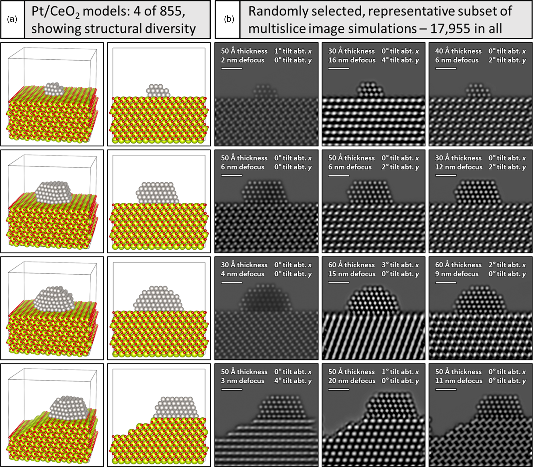
Fig. 1. Generating a large training dataset through multislice image simulation. Under (a) four (of 855) models are shown in a tilted view to emphasize the 3D structure (far left) and in a projected view along the electron beam direction (second column). Pt atoms are shown in gray, O atoms in red, and Ce atoms in yellow-green. A simulated image of every structure was generated for defocus values spanning 0–20 nm, resulting in 17,955 total images. Beneath (b), a representative subset of simulated images from each model is shown, with imaging conditions given in the figure inset (see text for more details). Scale bars in (b) correspond to 1.0 nm.
CNN Training and Testing
Before application to the experimental data, the networks were trained and evaluated on various subsets of simulated images. As will be discussed below, typically around 5,500 simulated images were used to train the network, with 550 other images randomly selected for validation and testing. Noisy data for training and evaluating the network were generated from clean simulated images by artificially corrupting the clean simulations with Poisson shot noise. That is, a noisy simulated image was produced pixel-wise by randomly sampling a Poisson distribution with a mean value equal to the intensity in the corresponding pixel of the clean ground truth image. We have verified that the noise in the experimental counted TEM image time series follows a Poisson distribution (see Supplemental Appendix B and Fig. S15), which is expected given the physical origin of the shot noise in the electron counted image acquisition process.
The network training process involves (1) applying artificial Poisson shot noise to a clean ground truth simulation, (2) denoising the noisy image with the neural network, (3) comparing the network-denoised image to the clean ground truth through a quantitative loss function, and (4) adjusting the parameters of the network iteratively to achieve better performance. The parameters are adjusted via back-propagation using the stochastic gradient descent algorithm (Goodfellow et al., Reference Goodfellow, Bengio and Courville2016). Periodically, the network is evaluated on a validation set of images not included in the training set. We chose to quantify the difference between the output and the ground truth by computing the L2 norm or mean squared error (MSE) of the two images, as is standard in the denoising literature. The magnitude of this value is conveniently represented by a related quantity known as the peak signal-to-noise ratio, or PSNR, which can be calculated from the MSE by the following equation:
 $${\rm PSNR} = 10\;\times \log _{10}\left({\displaystyle{{{\rm MAX}_I^2 } \over {{\rm MSE}}}} \right)$$
Here, MAXI is the maximum intensity value in the clean ground truth image. The PSNR is essentially a decibel-scale quantity that is inversely proportional to the MSE: a very noisy image will have a low PSNR. The PSNR for the noisy images in this work is around 3 dB. As is standard in the denoising literature, we choose to compare the denoising performance using the PSNR (which is derived from the MSE) rather than the MSE itself, in order to normalize against the range of the signal and provide a metric that is meaningful to the broader community.
It is desirable to investigate the performance of the network when applied to images that differ from the training data. We evaluated this so-called generalization ability along three different criteria: (1) the character of the atomic column contrast, (2) the structure/size of the supported Pt nanoparticle, and (3) the nonperiodic defects present in the Pt surface. To do so, the entire training dataset was divided into subsets based on the different categories of the three criteria. For example, for the atomic column contrast, the entire training dataset was split into three categories: white, black, and intermediate/mixed, largely based on the Pt and Ce atomic column intensities (see, e.g., Supplemental Fig. S1). After splitting the dataset into these subsets, the network was trained on one of them, and then systematically evaluated on the rest. So, for example, the network was trained on images from the white contrast category and then evaluated on images from either the black or intermediate/mixed contrast category. In these cases, the number of images in each training subset was set equal to establish a fair assessment. Additionally, the nanoparticle structures were classified into four categories, “PtNp1” through “PtNp4”, each with different size and shape, in accordance with the models displayed in Supplemental Figure S11. Finally, the defects were divided into five categories: “D0”, “D1”, “D2”, “Dh”, and “Ds”, in accordance with the models presented in Supplemental Figure S12.
All networks (e.g., the proposed architecture as well as those used in the baseline evaluation methods described below) were trained on 400 × 400 pixel-sized patches extracted from the training images and augmented with horizontal flipping, vertical flipping, random rotations between −45° and +45°, as well as random resizing by a factor of 0.955–1.055. The models were trained using the Adam optimizer (Kingma & Ba, Reference Kingma and Ba2015), with a default starting learning rate of 1 × 10⁻³, which was reduced by a factor of two each time the validation PSNR plateaued. Training was terminated via early stopping, based on validation PSNR (Goodfellow et al., Reference Goodfellow, Bengio and Courville2016).
The proposed network architecture is a modified version of U-Net (Ronneberger et al., Reference Ronneberger, Fischer, Brox, Navab, Hornegger, Wells and Frangi2015) with six scales to achieve a large field of view (roughly 900 × 900 pixels). Each convolutional layer contains 128 base channels (i.e., filters). Alternative architectures with differing numbers of scales and base channels were investigated. Increasing the number of base channels has a weak impact on performance—the number of scales (i.e., the number of down-sampling layers, which largely determines the network's receptive field) is much more important to obtaining good denoising performance, as discussed in Performance of Trained Network on Validation Dataset of Simulated Images section. The proposed network consists of six scales, each consisting of a down-block and an up-block. A down-block consists of a max-pooling layer, which reduces the spatial dimension by half, followed by a convolutional-block (conv-block). Similarly, an up-block consists of bilinear up-sampling, which enlarges the size of the feature map by a factor of two, followed by a conv-block. Each conv-block itself consists of conv–BN–ReLU–conv–BN–ReLU, where conv represents a convolutional layer, BN represents a batch normalization process (Ioffe & Szegedy, Reference Ioffe and Szegedy2015), and ReLU represents a nonlinear activation by a rectified linear unit. Further details on the alternative architectures tested, as well as a discussion on the associated design choices, are given in Mohan et al. (Reference Mohan, Manzorro, Vincent, Tang, Sheth, Simoncelli, Matteson, Crozier and Fernandez-Granda2020b).
Baseline Methods for Denoising Performance Evaluation
A number of other methods, including other trained denoising neural networks that are typically applied to natural images, were also applied both to the simulated and the real data in order to establish a baseline for evaluating the performance of the proposed network. A brief overview of the methods will be given here. The performance of the methods was compared quantitatively in terms of PSNR and structural similarity index measure (SSIM), which is a perceptually relevant metric for determining the similarity of two images based on the degradation of structural information, as explained in further detail in Wang et al. (Reference Wang, Bovik, Sheikh and Simoncelli2004).
(a) Adaptive Wiener filter (WF): An adaptive low-pass Wiener filter was applied to perform smoothing. The mean and variance of each pixel were estimated from a local circular neighborhood with a radius equal to 13 pixels.
(b) Low-pass filter (LPF): A linear low-pass filter with cut-off spatial frequency of 1.35 Å−1 was applied to preserve information within the ETEM instrumental resolution while discarding high-frequency noise.
(c) Variance stabilizing transformation (VST) + nonlocal means (NLM), or block-matching and 3D filtering (BM3D): NLM and BM3D are commonly used denoising routines for natural images with additive Gaussian noise (Buades et al., Reference Buades, Coll and Morel2005; Makitalo & Foi, Reference Makitalo and Foi2013). Here, a nonlinear VST (the Anscombe transformation) was used to convert the Poisson denoising problem into a Gaussian denoising problem (Zhang et al., Reference Zhang, Zhu, Nichols, Wang, Zhang, Smith and Howard2019). After applying the Anscombe transformation, we apply BM3D or NLM to the transformed image and finally use the inverse Anscombe transformation to recover the denoised image.
(d) Poisson unbiased risk estimator + linear expansion of thresholds (PURE-LET): PURE-LET is a transform-domain thresholding algorithm adapted to mixed Poisson–Gaussian noise (Luisier et al., Reference Luisier, Blu and Unser2011). The method requires the input image to have dimensions of the form (2n, 2n). To apply this method here, 128 × 128 pixel-sized overlapping patches were extracted from the image of interest, denoised individually, and finally stitched back together by averaging the overlapping pixels.
(e) Blind-spot denoising: We trained a blind-spot network based on U-net, as developed by Laine et al. (Reference Laine, Karras, Lehtinen and Aila2019). Here, training was done using 600 × 600 pixel-sized patches from the images of interest. The Adam optimizer was used with a starting learning rate of 1 × 10⁻⁴, which was reduced by a factor of two every 2,000 epochs. Overall, the training proceeded for a total of 5,000 epochs.
(f) Denoising convolutional neural network (DnCNN): Following the protocol outlined in the Convolutional Neural Network Training and Testing section, we trained the DnCNN model as described previously by Zhang et al. (Reference Zhang, Zuo, Chen, Meng and Zhang2017).
(g) Small U-Net from dynamically unfolding recurrent restorer (DURR): Following the protocol outlined in the Convolutional Neural Network Training and Testing section, we trained a U-Net architecture implemented in the DURR denoiser proposed by Zhang et al. (Reference Zhang, Lu, Liu and Dong2018).
Aside from these methods, standard filtering techniques including Gaussian blurring, median filtering, and Fourier transform (FT) spot-mask filtering were applied using routines built-in to the ImageJ analysis software (Schneider et al., Reference Schneider, Rasband and Eliceiri2012). Where relevant, additional details will be given to aid in understanding.
Results and Discussion
Need for Improved Denoising Methods and Overview of CNN-Based Deep Learning Denoiser
A single 25 ms exposure counted frame of a CeO2-supported Pt nanoparticle from an experimentally acquired time-resolved in situ TEM image series is presented in Figures 2a1 and a2. The Pt particle is in a [110] zone axis on a [111] CeO2 surface that is itself in a [110] zone axis orientation. These orientation relationships and particle/support zone axes were commonly encountered during the experiment. Even though a relatively high dose rate of 5 × 10³ e−/Å2/s was used to acquire the image series, for time-resolved frame rates on the order of ms, many of the pixel values are zero. In the present case, the average electron dose counted in the vacuum region of the image is 0.45 e−/pixel/frame. Following Poisson statistics, wherein the variance of the signal is equal to the mean value, and assuming the intensity in the vacuum region is uniform, the signal-to-noise ratio (SNR) of the incident beam is only SNR =  $ 0.45/\sqrt {0.45} = \sqrt {0.45} = 0.67 < 1$. Hence, the image is severely degraded by shot noise. The impact of the shot noise limitation is emphasized by magnifying the region marked by the dashed white box, which is presented in Figure 2a2. Here, the quality of the signal is appreciably low, and the Pt atomic columns at the nanoparticle surface are hardly discernible.
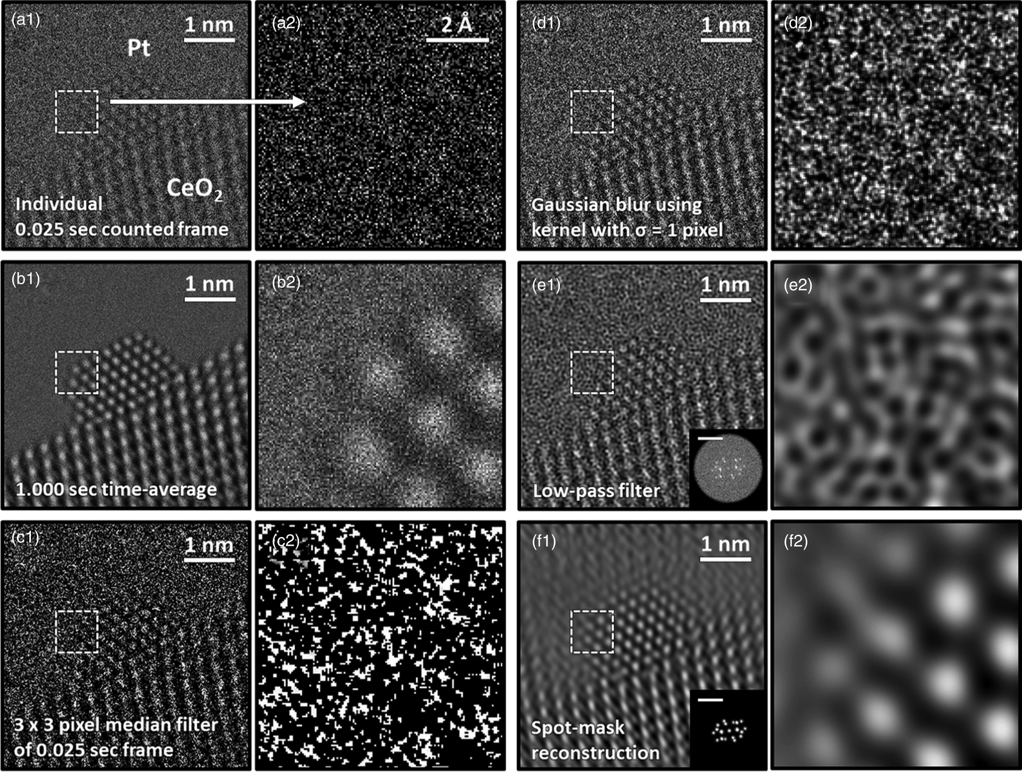
Fig. 2. Comparison of typical processing techniques applied to an ultra-low SNR experimental TEM image of a CeO2-supported Pt nanoparticle. In (a1), an individual 0.025 s counted frame is shown along with (a2) a zoom-in image taken from the region designated by the dashed box. In (b), a 1.000 s time-averaged image is shown; (c) displays the result of filtering the frame with a 3 × 3 pixel median filter; (d) displays the result of filtering the frame with a Gaussian blur with standard deviation equal to 1 pixel; (e) shows a Fourier reconstruction of the individual frame after applying a low-pass filter up to the 0.74 Å information limit, with the FT given in the inset along with a 1 Å−1 scale bar; and (f) displays another Fourier reconstruction acquired through masking the Bragg beams in the diffractogram, as shown in the figure inset.
One common approach to improving the SNR of time-resolved image series involves aligning and then summing together nonoverlapping groups of sequential frames, yielding a so-called time-averaged or summed image. Figure 2b1 presents a 1.000 s time-averaged image produced from adding together 40 sequential 0.025 s frames. The pronounced improvement in SNR, which has increased by a factor of  $\sqrt {40} = 6.32$ to SNR = 4.24, is readily evident, as seen by the well-defined and bright atomic columns that appear in Figure 2b2.
Increasing the SNR without time-averaging can be accomplished by applying linear or nonlinear filters that act on variously sized and/or distributed domains in real or frequency space to remove sharp features arising from high noise content. The result of applying a nonlinear median filter with a 3 × 3 pixel-sized kernel to the noisy single frame is presented in Figure 2c. The application of a linear Gaussian blur with a kernel that has a standard deviation equal to 1 pixel yields the filtered image presented in Figure 2d. Applying kernels of these sizes and characters produced the best improvement in image quality for each filter. Although the filtered images appear smoother and offer an enhanced visualization of the atomic columns in comparison to the raw image, the action of the filters also introduces artifacts to the signal, which can complicate a precise analysis of the atomic column position and/or intensity.
Working in reciprocal space through the application of an FT allows one to consider spatial frequency filters that exclude components attributable to noise, with a subsequent reconstruction of the image using the desired domains from the filtered FT. Figure 2e1 presents a Fourier reconstruction of the individual frame after applying a linear low-pass filter that excludes components with spatial frequencies beyond the instrument's 1.35 Å−1 information limit. After eliminating the high-frequency information corresponding to noise, the contrast in the image exhibits an unusual texture that hinders feature identification, as seen in Figure 2e2. Figure 2f displays another Fourier reconstruction produced by spot-masking the regions corresponding to Bragg beams in the FT, as presented in the figure inset. Although this reconstructed image offers an improved SNR compared to the raw frame and even to the other filtering techniques, the procedure introduces severe ringing lattice-fringe artifacts into the vacuum region and at the nanoparticle surface, making it unacceptable for use in the study of defects or aperiodic structures.
There is a pressing need for improved denoising techniques that both preserve the high time resolution of the original data and also facilitate the retrieval of nonperiodic structural features, e.g., nanoparticle surfaces and atomic-level defects. Toward this end, we develop a deep CNN that is trained on a big dataset of simulated TEM images before being applied to real data.
A schematic overview of the deep CNN training, application, and evaluation process is provided in Figure 3. During training (top), a large dataset of noisy simulated images is given to the network. Noisy images were generated from clean simulated images by corrupting them with Poisson shot noise. For each noisy image, the network produces a prediction of the underlying signal, effectively denoising the image. The denoised prediction is compared to the original clean simulation by computing the L2 norm between the two images. Better denoising performance is achieved by iteratively adjusting the parameters within the network in order to minimize the difference between the denoised output and the original simulation.
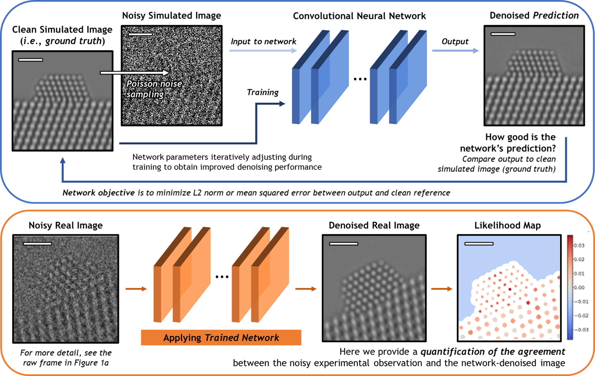
Fig. 3. Overview of the deep CNN training, application, and evaluation process. (Top) The network is trained on a large dataset of noisy multislice TEM image simulations; the denoised prediction output by the network is compared to the original clean image simulation through a loss function based on the L2 norm (i.e., mean squared error). The parameters in the network are iteratively adjusted to minimize the magnitude of the loss function. (bottom) The network trained on simulated images is then applied to real experimental data taken under similar imaging conditions. The performance of the network on real images lacking noise-free counterparts can be evaluated through a statistical likelihood analysis, which allows one to quantify the agreement between the denoised image and the noisy experimental observation. All scale bars correspond to 1.0 nm.
After successfully training the network, it may be applied to real data (bottom). The denoised experimental 25 ms frame produced by the network presents a significant improvement in SNR without temporal averaging and without making sacrifices to the study of nonperiodic structural features. However, given the high level of noise present in the raw data, caution must nonetheless be exercised when performing analysis on the network-denoised output. As will be shown, we have established an approach for quantifying the degree of agreement between the network estimated output and the noisy raw input, which takes the form of a statistical likelihood map.
Performance of Trained Network on Validation Dataset of Simulated Images
Before applying the trained network to real data, it is important to assess and validate the network's performance on noisy simulated data that it has not seen before. Figure 4 presents a representative comparison of the surveyed methods against our proposed network on an image randomly selected from the validation dataset. A similar comparison for another randomly selected image in the validation dataset is given in Supplemental Figure S2. The aggregate performance, in terms of PSNR and structural similarity [SSIM (Wang et al., Reference Wang, Bovik, Sheikh and Simoncelli2004)], for each denoising approach over all images in the validation dataset is summarized in Table 1. Descriptions of each method are given in detail in Baseline Methods for Denoising Performance Evaluation section. The noisy simulated image shown in Figure 4a, along with the zoom-in image taken from the region indicated by the red box along the Pt nanoparticle surface, illustrating the severity of the signal degradation that has occurred due to shot noise. The same noisy image was processed using the denoising methods described in Baseline Methods for Denoising Performance Evaluation section. The results are presented in Figures 4b–4i in order of increasing performance in terms of PSNR. The original ground truth simulated image, which serves as a ground truth reference, is presented in Figure 4j.
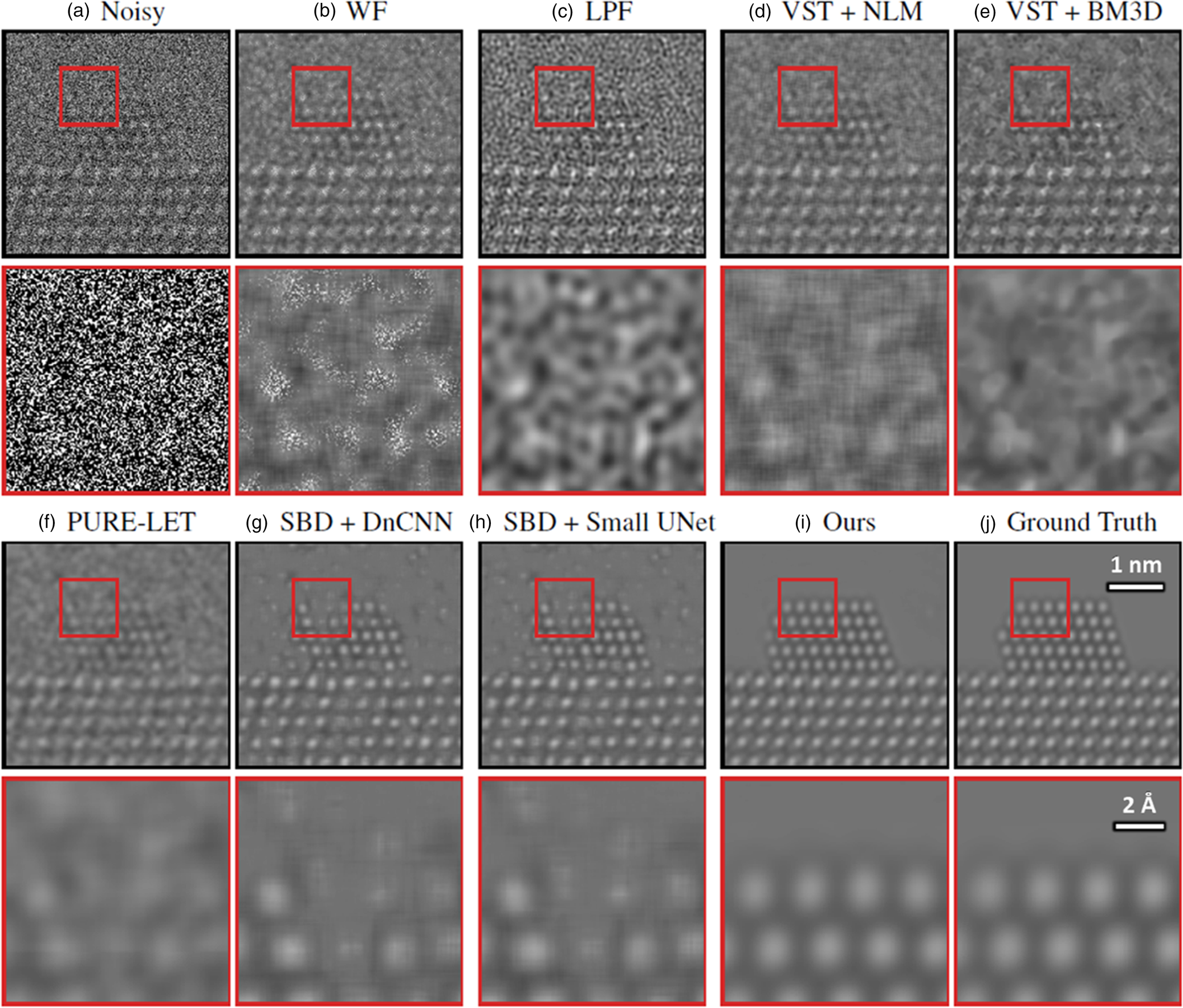
Fig. 4. Comparing the proposed network's performance on multislice simulations against other baseline denoising methods, including other neural networks. See text for an explanation of the methods. In brief, (a) displays a noisy simulated image, along with a zoom-in on the region indicated by the red box in the figure inset. (b) through (i) show the outputs from the networks listed in Table 1. The clean simulated image is shown as a ground truth reference in (j). The proposed network produces denoised images of high quality, recovering precisely the structure of the nanoparticle, even at the surface, with comparatively few artifacts, as shown in (i).
Table 1. Summary of Denoising Performance on Simulated Images in Terms of Mean PSNR and SSIM, Along with the Standard Deviation, for Each of the Surveyed Methods Aggregated Over All of the Images in the Validation Dataset.
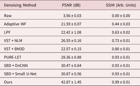
In general, the proposed deep CNN denoising architecture outperforms the baseline methods by a large margin, achieving a PSNR of 42.87 ± 1.45 dB and an SSIM of 0.99 ± 0.01. The starting PSNR of the noisy simulation is about 3 dB. As seen in Figure 4i, the proposed network produces an estimated image that closely resembles the ground truth simulation. In addition to recovering the overall shape of the Pt nanoparticle, the aperiodic structures of the Pt surface and the Pt/CeO2 interface, as well as the subtle contrast variations that are present in the CeO2, have all been accurately denoised by the proposed architecture. The next-best performance is attained by the other two simulation-based denoising (SBD) neural networks (e.g., Figs. 4g, 4h), which reach PSNR and SSIM values around 30.6 dB and 0.93, respectively. However, in the images denoised through these inferior networks, the contrast features around aperiodic sites or abruptly terminating surfaces are typically missing or distorted. Moreover, significant artifacts often appear in these images, including phantom atomic column-like contrast in the vacuum, or unrealistic structures characterized by missing columns in unphysical sites, e.g., the material bulk.
A number of decisive factors contribute to the performance of the network. First is the size of the network's receptive field. The receptive field is the region of the noisy image that the network can see while estimating the intensity of a particular denoised output pixel. The receptive field is not equivalent in size to the region of the image input to the network but rather is determined by the number and dimension of consecutive convolution and down-sampling operations performed by the network. Further details on the concept can be found in the literature (Goodfellow et al., Reference Goodfellow, Bengio and Courville2016; Araujo et al., Reference Araujo, Norris and Sim2019). The baseline networks evaluated in the performance comparison, which are the present state-of-the-art in denoising natural images, employ receptive fields either 41 × 41 pixels (in the case of DnCNN, Fig. 4g) or 45 × 45 pixels (in the case of the small U-Net, Fig. 4h). Given the fact that the real space pixel size of the data is 6.1 pm, these receptive fields amount to regions around 0.26 nm × 0.26 nm in size. As shown in Supplemental Figure S3, with a limited receptive field of such size, it is challenging to see the structure of the atomic columns in the ground truth simulation. Once shot noise has been added to reduce the PSNR to 3 dB, differentiating regions containing structure from those which contain only vacuum becomes virtually impossible by eye. Increasing the receptive field is critical to achieving better denoising performance. Supplemental Figure S4 shows that expanding the receptive field by a factor of 25 to a region around 200 × 200 pixels (i.e., 1.22 nm × 1.22 nm) allows the network to sense the local structure around the pixel to be denoised. With a receptive field of this size, different structures (e.g., vacuum, Pt surface, CeO2 bulk, surface corner site) remain discernible even after adding noise. This suggests that increasing the receptive field contributes to the network's ability to detect subtle contrast variations as well as aperiodic defects. In this work, the network's receptive field was increased simply by implementing aggressive down-sampling. The receptive field of the proposed network is roughly 900 × 900 pixels (i.e., 5.49 nm × 5.49 nm, Fig. 4i).
The network's performance is also influenced by the nature of the images contained in the training dataset. Here we have discovered that the geometry of the image (i.e., the scaling and orientation), as well as the character of the atomic column contrast (i.e., the focusing condition), appear to have the largest impact on performance. In Supplemental Figure S5, we demonstrate that the denoising performance measured in terms of PSNR degrades significantly when the network is evaluated on simulated images that have been scaled or rotated in a manner that was missing from the images in the training dataset. Note that the performance remains roughly constant across various values of pixel size and orientation when these pixel sizes and orientations are present in the training dataset. These results indicate that augmenting the training data with random resizing/rotations can ensure that robust performance is obtained when the network is applied to real data, which may differ slightly in exact scaling or orientation from the images in the training dataset. Practically, the results also imply that networks must be carefully trained to denoise images taken at the particular image magnification of interest.
We have also investigated the generalizability of the network to unseen supported nanoparticle structures, non-periodic surface defects, and atomic column contrast conditions (i.e., defocus). As shown in Supplemental Figure S6, the network generalizes well to new (a) nanoparticle structures of various shape/size and (b) atomic-level Pt surface defects, with a good and consistent PSNR denoising performance above 34 dB for all of the categories explored here. The network is also generally robust to ±5 nm variations in defocus. The largest degradation in performance (PSNR = 28 dB) is observed when the network is trained on images with black-column contrast and tested on images with white-column contrast. A general conclusion would be to train the network using images simulated at a defocus close to the data that are to be denoised.
Evaluating the Network's Ability to Accurately Predict Nanoparticle Surface Structure
Understanding the atomic-scale structure of the catalyst surface is of principal scientific interest. Here, we perform a detailed evaluation of the network's ability to produce denoised images that accurately recover the atomic-level structure of the supported Pt nanoparticle surface. The analysis was conducted over a set of 308 new simulated images that were specifically generated for the surface structure evaluation. A series of 44 Pt/CeO2 structural models were created with many different types of atomic-level surface defects, including, e.g., the removal of an atom from a column, the removal of two atoms, the removal of all but one atom, the addition of an adatom at a new site, etc., to emulate dynamic atomic-level reconfigurations that could potentially be observed experimentally. Nine of the models are shown in Supplemental Figure S7 to provide an overview of the type of surface structures that were considered. Images were simulated under defocus values ranging from 6 nm to 10 nm, all with a tilt of 3° in x and −1° in y and a support thickness of 40 Å. Note that these images were never seen by the network during the training process and demonstrate an evaluation of its performance on unseen images.
A ground truth simulated image from the surface evaluation dataset is shown in Figure 5a1. A so-called blob detection algorithm based on the Laplacian of Gaussian approach was implemented to locate and identify the Pt atomic columns in the image (Kong et al., Reference Kong, Akakin and Sarma2013). Each of the 308 sets of identified atomic columns were compared to their corresponding clean images and inspected for errors; no discrepancies were found. The atomic columns at the nanoparticle surface were distinguished from those in the bulk by computing a Graham scan on the identified structure (Graham, Reference Graham1972). Figure 5a2 shows a binary image depicting the Pt atomic columns identified in one of the ground truth simulated images. The set of atomic columns located at the surface have been highlighted with a green line.
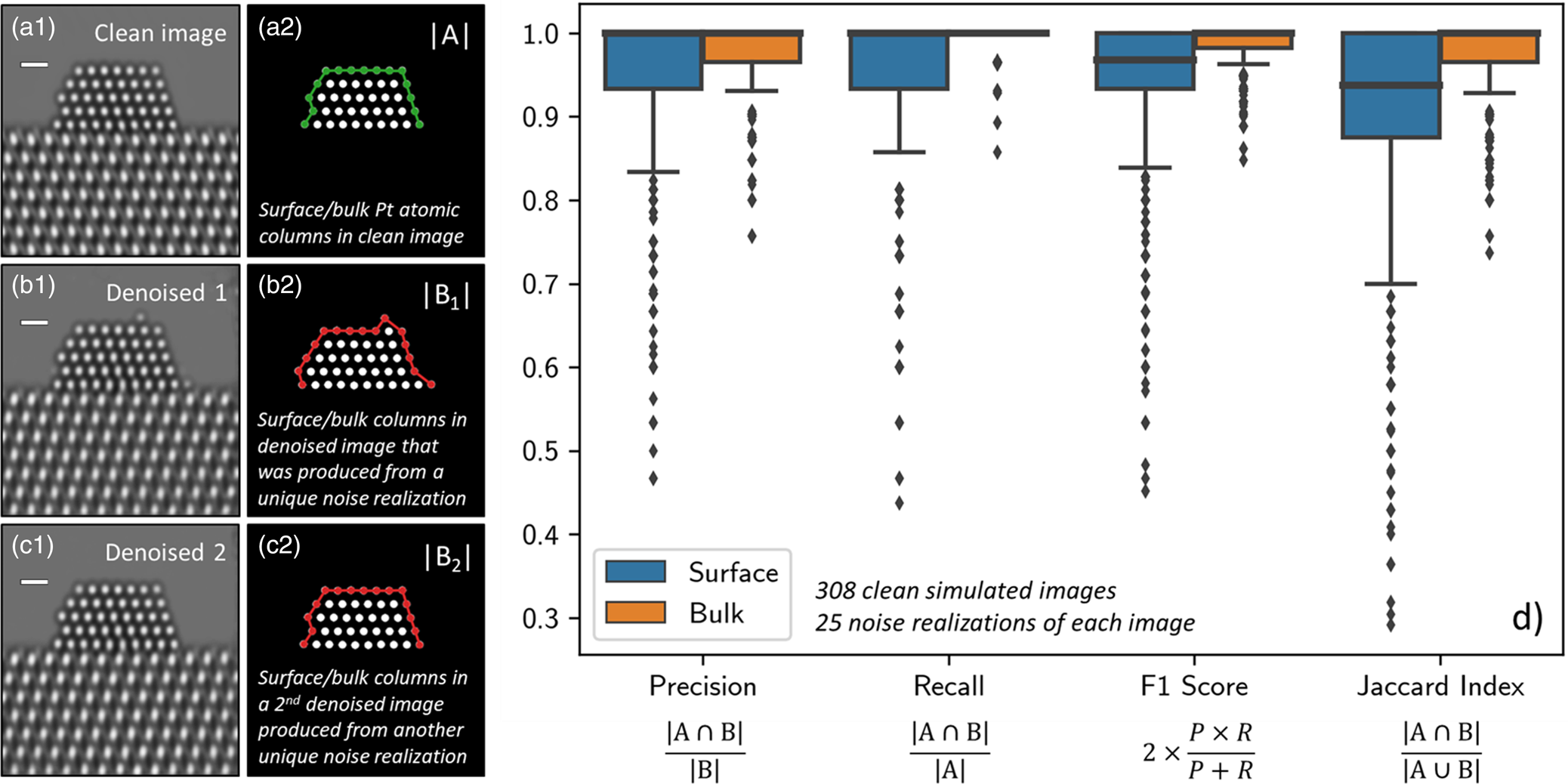
Fig. 5. (a1) depicts a representative ground truth simulation from the Pt atomic structure evaluation image dataset (n ground truth = 308). To the right, in (a2), the set of Pt columns identified in the ground truth image (i.e., |A|) are shown, with those located at the surface highlighted by a green line. (b1) and (c1) show two denoised images produced by the network from two unique noise realizations of the same original simulation. To the right, in (b2) and (c2), the set of Pt columns identified in the respective denoised images (i.e., |B|) are shown, with those at the surface highlighted now by a red line. To quantify the network's performance in recovering the Pt atomic structure, we compute the precision, recall, F1 score, and Jaccard index of the two sets. (d) provides box plot distributions of each metric for both the surface (blue boxes) and the bulk (orange boxes) computed over 25 noise realizations of each ground truth simulation (n denoised = 7,700). Outliers in the distributions are marked by small diamonds. Scale bars in (a1)–(c1) correspond to 5 Å.
Evaluating the network's ability to recover surface structure can be accomplished by examining how this set changes after denoising. Figure 5b1 displays a denoised image produced by the network from a unique Poisson noise realization of the ground truth simulation. While the network denoises with outstanding performance and recovers the overall shape of the specimen, note the appearance of the three spurious Pt surface atomic columns that do not appear in the original ground truth simulation. The Pt atomic columns identified in this denoised image are pictured in Figure 5b2, where those located at the surface are highlighted now by a red line. The spurious Pt surface atomic columns have been marked with white arrows. Based on inspection of the noisy data, we believe that the particular distribution of intensity present in the noise realization can lead the network to produce denoised estimates with spurious surface atoms, perhaps due to the random clustering of intensity in a manner that appears to resemble an atom (see, e.g., Supplemental Fig. S8). Figure 5c1 displays a denoised image produced by the same network from a second unique Poisson noise realization. Note that in this case, the Pt surface structure has been recovered exactly. The Pt atomic columns identified in this denoised image are pictured in Figure 5c2 and are equivalent to those identified in the original simulation.
To quantify the network's performance in recovering the Pt atomic structure, we compute four metrics that are commonly employed in the field of machine learning: precision, recall, F1 score, and Jaccard index. These metrics are defined by the following equations:
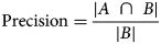 $${\rm Precision} = \displaystyle{{\vert {A\;\cap \;B} \vert } \over {\vert B \vert }}$$
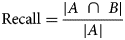 $${\rm Recall} = \displaystyle{{\vert {A\;\cap \;B} \vert } \over {\vert A \vert }}$$
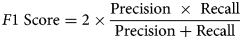 $$F1\;{\rm Score} = 2 \times \displaystyle{{{\rm Precision}\;\times \;{\rm Recall}} \over {{\rm Precision} + {\rm Recall}}}$$
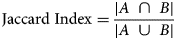 $${\rm Jaccard\;Index} = \displaystyle{{\vert {A\;\cap \;B} \vert } \over {\vert {A\;\cup \;B} \vert }}$$
These metrics were calculated for both the surface and the bulk structure; when the metrics were calculated for the surface structure, |A| represents the set of Pt atomic columns identified at the surface in the ground truth simulation, and |B| represents the columns identified at the surface in the denoised image. Similarly, when the metrics were calculated for the bulk structure (i.e., everything other than the surface), |A| and |B| represent the bulk atomic columns in the ground truth and denoised images, respectively. To attain an accurate representation of the network's performance, 25 noise realizations of each ground truth simulation were sampled and then denoised, resulting in an evaluation over 7,700 total images.
Figure 5d displays box plot distributions of the four metrics computed over all 7,700 images for both the surface (blue boxes) and the bulk (orange boxes). Box plots, or box-and-whisker plots, are useful for graphically visualizing distributions of data on the basis of the quartiles that exist within the distribution. The quartiles are a set of three numerical values that divide the number of data points in the distribution into four roughly equally sized parts; e.g., the second quartile is the median or mid-point of the dataset when the values are ordered from smallest to largest, the first quartile lies halfway between the smallest value and the median, and the third quartile lies halfway between the median and the largest value. In the box-and-whisker plot, the box is drawn from the first quartile (Q1) to the third quartile (Q3) with the median value represented by a line within this box. Whiskers, which are lines extending beyond the edges of the box, can be useful for describing the behavior of the data that falls in the upper or lower quartile of the distribution. Here we choose to follow a standard practice for drawing the whiskers: a distance equal to 1.5× the interquartile range (defined by Q3–Q1) is drawn from each edge of the box; on the top of the box, for example, the largest value above Q3 that lies within this distance is defined as the edge of the top whisker; similarly, the smallest value below Q1 that lies within this distance is defined as the edge of the bottom whisker. Values beyond the edge of the whiskers are considered outliers; here, they are drawn as small solid diamonds. As seen in Figure 5d, the box plots for the bulk are all narrow and have median values of 1.0, which is expected given that the network was not seen to produce images characterized by unphysical bulk structures, such as, e.g., missing interior atomic columns.
The distributions for the surface structure are slightly more varied and reveal detailed information about the performance of the network. First, consider the distribution for the precision (left-most box plot in Fig. 5d). The precision, or the positive predictive value, measures the fraction of real surface columns over all of the surface columns identified in the denoised image. Effectively, a lower precision value indicates that there are more false positives (i.e., spurious surface columns) in the denoised output. As a reference, consider a ground truth simulation in which there are originally 15 atomic columns present at the surface (e.g., Fig. 5a1). The addition of one spurious surface column would result in a precision value of 0.93, while the addition of three columns would yield a precision value of 0.80. As seen in Figure 5d, the median precision value is 1.0 and the first quartile lies nearby at 0.93. Thus, the precision distribution shows the network frequently produces denoised images that do not contain spurious atomic columns; occasionally it will include one, and rarely it will add two or more.
In addition to including spurious atomic columns, the network may fail to recover the full structure, resulting in a real column that is absent from the denoised image. The prevalence of this event can be captured by the recall, which measures the fraction of real columns over all of the columns identified at the surface in the clean ground truth image. Effectively, a lower recall value indicates that there are more false negatives in the network-denoised output, which means that columns which were originally present in the ground truth image are no longer present in the network-denoised output. As presented in Figure 5d, the median recall value is also 1.0, with a distribution that is similar to—but narrower than—the precision. These values again indicate an impressive performance by the network. Interestingly, the slightly smaller distribution suggests that the network may tend to include spurious atomic columns more often than it fails to sense real atomic columns.
Taking the harmonic mean of the precision and recall yields the F1 score, which accounts both for false positives as well as false negatives. Here, the median value of the F1 score distribution is around 0.96, and the first quartile lies around 0.93. Given that the median precision and recall are both 1.0, it is not surprising that the F1 score distribution is also narrow and clustered around high values (i.e., greater than 0.90). Note that the harmonic mean of 1.0 (the median precision/recall) and 0.93 (the first quartile of both distributions) equals 0.96, which is the median F1 score. Thus, the F1 score reveals that while the network may occasionally include a spurious column or fail to include a real one, combinations of these errors occur less frequently.
Finally, we have computed the Jaccard index to gauge the exact degree of similarity between the surface structure in the clean and denoised images. As defined above, the Jaccard index equals the fraction of true positives (i.e., real columns) over the union of surface columns identified in both the clean and the denoised images. The ideal value of 1.0 occurs only when the exact atomic structure is recovered. In general, for the images in the surface evaluation dataset, the addition of a spurious atomic column would give a Jaccard index of 0.87, while the omission of a real column would give a value of 0.93. The distribution plotted in Figure 5d shows that the median Jaccard index value is 0.93 and that the first quartile lies at 0.87. Observe that the third quartile lies at 1.0, signaling that the network will achieve a perfect performance in recovering the precise atomic structure at the surface at least 25% of the time, despite the extreme degree of signal degradation that has occurred due to shot noise. The location of the first quartile at 0.87 indicates that at least 66% of the errors involve the addition or omission of only one atomic column. The remaining errors, which represent at most 25% of the total data, involve the addition and/or omission of more than one atomic column. Further studies implementing this approach could be done in the future to assess the effect that varying the noise level has on the network's ability to predict the atomic-level surface structure exactly.
Quantifying the Agreement Between the Noisy Observation and the Network-Denoised Output
When applying the trained network to real data, the atomic structure in the network-denoised output cannot be compared to a clean ground truth image, since none is available. Establishing a tool to assess the likelihood of an atomic column's appearance in the network-denoised image would thus be of great utility. Here, we develop a statistical analysis based on the log-likelihood ratio test that makes it possible to hypothetically evaluate whether an atomic column in the denoised image is (1) likely to represent a true atomic column in the structure or (2) likely to be an artifact introduced by the denoising neural network. Additionally, a graphical visualization of the log-likelihood ratio is created in the form of a likelihood map. The log-likelihood ratio method requires only the network-denoised image and the noisy input and is therefore extensible to real experimental data, where no clean ground truth references exist.
First, we validate the analysis on a large dataset of simulated images, for which the true atomic structures are exactly known. Figure 6 depicts a representative (a) noisy and (b) denoised image from the simulated dataset discussed in the prior section. To compute the log-likelihood ratio and generate the likelihood map, the following procedure is implemented: first, an atomic column in the denoised image is located, e.g., through blob detection, as was done in the previous section (here, we focus on the Pt columns, although the method is generalizable to any area of interest so long as it can be identified in the denoised image). As a simplifying assumption, we model the intensity of the atomic column as a constant value, which is obtained by averaging over all the denoised pixels in the region R identified by the blob detection algorithm. We have investigated the impact on the likelihood from a fitted Gaussian shape, and it showed little difference from that calculated from averaging. Since there is no considerable advantage to fitting a Gaussian to the data, we choose not to do so for simplicity. Additionally, we assume that the signal within the atomic column region is constant in order to be consistent with the log-likelihood ratio test procedures. In Supplemental Figure S9, we show that for these imaging conditions, averaging over the column is a good assumption, provided the region R is restricted to a limited area (e.g., radius < 0.7 Å) within the innermost portion of the atomic column, where the intensity is largely invariant. This provides a directly interpretable metric that can be used to quantitatively evaluate the degree of consistency between the denoised output and the noisy raw data.
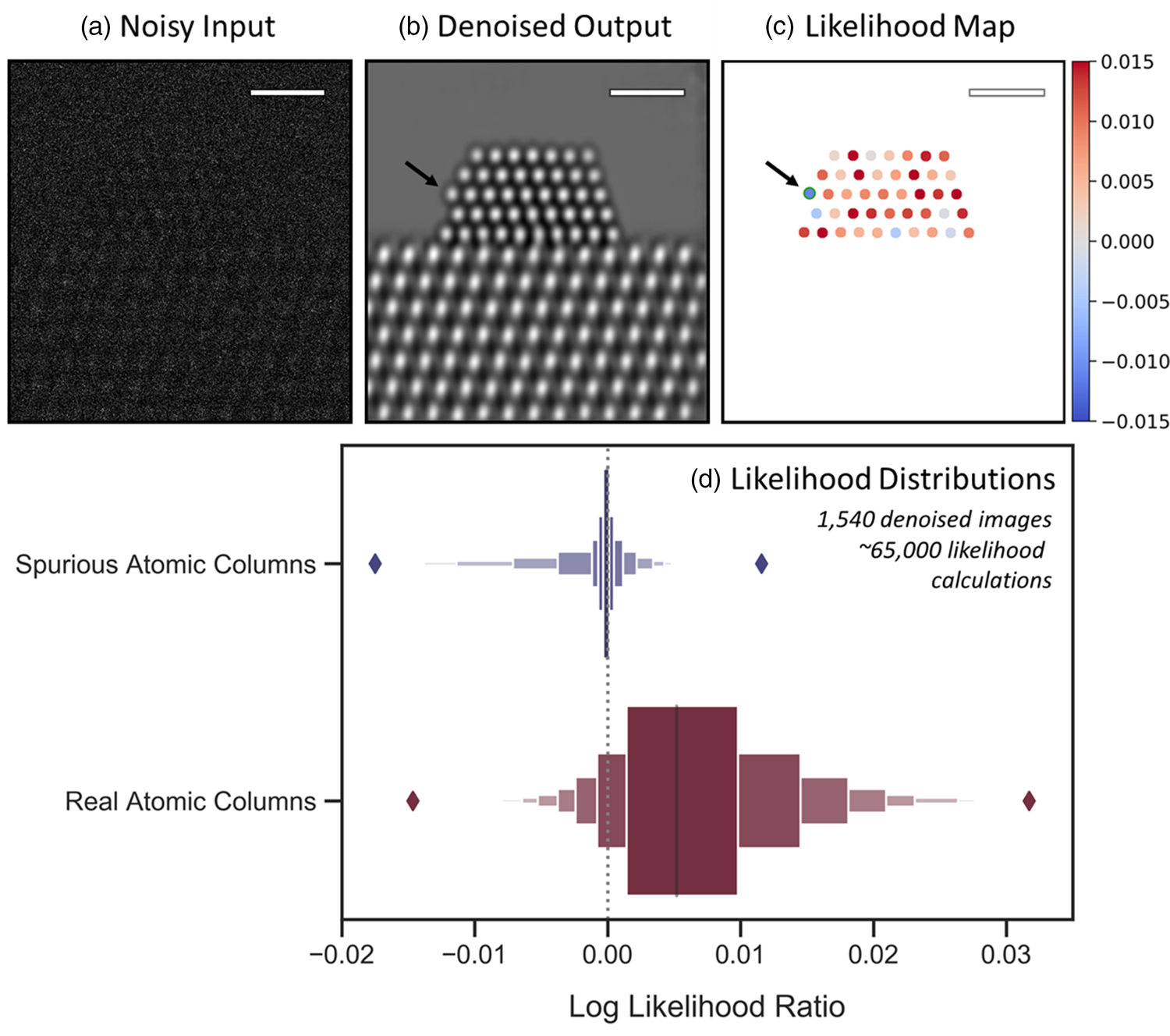
Fig. 6. Likelihood analysis to quantify the agreement between noisy data and network-denoised output. In (a), a representative noisy simulated image is shown along with (b) a denoised image output by the network. (c) depicts an atomic-level likelihood map, which visualizes the extent to which the atomic structure identified in the denoised image is consistent with the noisy observation. After denoising, a spurious atomic column appears at the arrowed site, which shows a large negative value in the likelihood map, indicating that the presence of an atomic column at this location is not likely. The likelihood analysis has been performed over 1,540 denoised images, yielding the distributions given by the letter-value plots for spurious (blue, top) and real (red, bottom) columns in (d). The diamonds mark the extrema of the two distributions. Scale bars in (a)–(c) correspond to 1.0 nm.
Second, we compute the statistical likelihood, L, of observing the noisy data in R of the input, assuming the true signal in this region is the constant value calculated from the denoised output. We know that the observed signal is governed only by shot noise, which can be modeled with a Poisson distribution. And furthermore, we assume that every pixel is mutually independent, so that the overall likelihood in R is simply the product of the individual probabilities for each pixel i in R. Mathematically, the likelihood calculation is then defined by the following equation:
 $$L( R ) = \mathop \prod \limits_{i\;\in \;R} \;p_\lambda ( {x_i} ) $$
where x i is the intensity of the ith noisy pixel in R, and  $p_\lambda$ is a Poisson probability mass function characterized by a mean of λ, which is equal to the constant value calculated from the denoised output. Here, a higher likelihood value would indicate a better level of agreement between the denoised output and the noisy data. To assess instead whether the column is an artifact of the denoising network, we also compute the likelihood of observing the noisy data in R with the true signal now represented by the constant value of the vacuum (i.e., λ = 0.45).
Comparing the relative magnitude of these two likelihood values allows one to consider whether the atomic column is likely to be real or spurious. How consistent either hypothesis is with the noisy observation can be tested by taking the natural log of the likelihood ratio (also known as a log-likelihood ratio test). Considering, e.g., the noisy and denoised images of Figures 6a and 6b, the results of this test are conveniently visualized for every atomic column detected in the denoised image through the likelihood map that is presented in Figure 6c. Positive (red) log-likelihood ratio values indicate the detected column is more consistent with the noisy data than is the presence of vacuum. Conversely, sites with negative (blue) values are less consistent with the data and may therefore be spurious additions. A spurious atomic column appears in this denoised image at the corner site marked by the black arrow on the left side of the particle. Observe that the likelihood map displays a relatively large negative value of −0.012 at this site, signaling that the detected atomic column is inconsistent with the noisy data and likely to be a spurious column.
It should be discussed that the likelihood map shows a handful of sites that correspond to real atomic columns, but which nonetheless have negative log-likelihood ratio values, including, e.g., in the bulk of the nanoparticle. First, we point out that the likelihood map does not provide an absolute validation of the structure present in the denoised image but rather offers a visualization of the statistical agreement between this structure and the noisy input. In this case, the observed image has been so degraded by shot noise (vacuum SNR = 0.67) that, inevitably, a few real atomic columns will be observed to have average noisy intensities that are more consistent with the vacuum level. The sensitivity of the log-likelihood ratio in response to the overall SNR has not been investigated and could be the subject of future work. As a second point, the appearance of real atomic columns with a negative log-likelihood ratio is in some way a testament to the network's ability to infer the presence of structure in spite of an SNR so low that the data appear more consistent with vacuum. This point is explored further in Performance on Experimental Data and Visualizing the Network's Effective Filter section. It is also worth pointing out that in a time series of images, one would be able to look at the variation in the likelihood map for different frames to facilitate a more correct interpretation.
Regardless of these nuances, some useful heuristics may still be established that allow one to use the likelihood map to quickly assess the atomic structure that appears in the denoised image. Figure 6d presents letter-value or so-called boxen plots of ~65,000 log-likelihood ratio values calculated over 1,540 denoised images (5 unique noise realizations of 308 ground truth images), providing insight into how the distribution of values derived from spurious atomic columns (top) compares with that derived from real atomic columns (bottom). A dashed vertical line is provided at 0.0 for reference. The spurious column distribution shows a slightly negative median and is clustered around 0.0 while being skewed toward negative values. The positive tail diminishes rapidly and becomes marginal for values above 0.0045. On the other hand, the real atomic column distribution has a positive median of 0.0052 and is skewed toward the right. Many values are seen to exceed 0.010, which virtually never occurs for spurious atomic columns. The negative tail becomes negligible for values below −0.0060. These distributions reveal two simple guidelines: (1) sites with log-likelihood ratio values ≥0.0050 can be treated as a real structure with a high degree of certainty, and (2) sites with log-likelihood ratios ≤−0.0060 (e.g., the spurious column arrowed in Fig. 6c) are almost certainly artificial. A site with a value in between is not as easily distinguishable but nonetheless still has a quantitative statistical measure of agreement given by its log-likelihood ratio. In principle, during general analysis, one could use the log-likelihood ratio information to evaluate various denoised structures that are more or less consistent with the noisy input. It is also worth noting that in practice additional prior information (e.g., knowledge of the material) may also be leveraged to support an assessment of the predicted structure.
Performance on Experimental Data and Visualizing the Network's Effective Filter
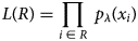
The trained network was applied to the experimentally acquired in situ TEM image dataset. Several other state-of-the-art denoising techniques were also applied to the same real data in order to establish a baseline for evaluating the performance of the proposed network. Figure 7 presents a summary of the results. A single 25 ms exposure in situ TEM image of a CeO2-supported Pt nanoparticle in 5 mTorr N2 gas is shown in Figure 7a. Beneath it, a zoom-in image is shown from the region marked by the red box at the Pt nanoparticle surface, to demonstrate the severity of the shot noise and the lack of clarity regarding the underlying image signal. Each baseline method was applied to the same noisy image, generating the denoised outputs shown from Figures 7b–7g. Details on all of the methods are given in Baseline Methods for Denoising Performance Evaluation section. The denoised image produced by the proposed network architecture is shown in Figure 7h. Although a clean reference image is not available experimentally, a relatively high SNR image has been prepared by time-averaging the experimental data over 40 frames for 1.0 s total, as shown in Figure 7i. Finally, Figure 7h displays the likelihood map for interpreting the structure that appears in the proposed network's output. The likelihood analysis was not applied to the images produced by the baseline methods, due to the abundance of obvious artifacts introduced by these methods, as discussed below.
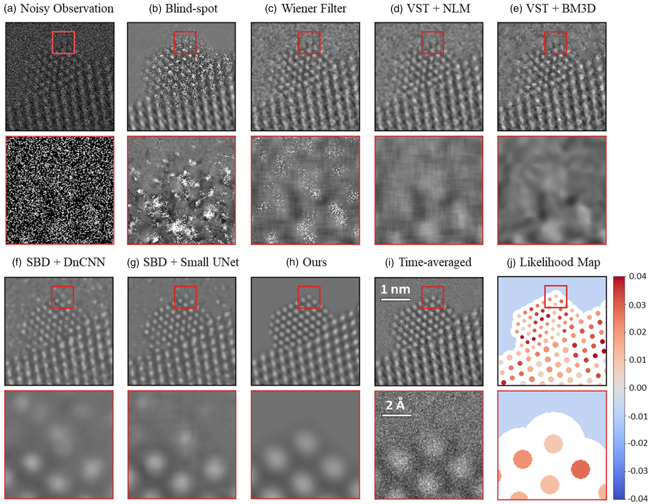
Fig. 7. Evaluating the performance of the proposed network on experimental 25 ms exposure in situ TEM images, in comparison to current state-of-the-art methodologies. A raw 25 ms frame of a CeO2-supported Pt nanoparticle in 5 mTorr N2 gas is shown in (a) along with a zoom-in image from the region marked by the red box. Denoised estimates of the same raw frame from the baseline methods are presented in (b) through (g), while (h) displays the denoised estimate from the proposed network. (i) presents a time-average over 40 raw frames, or 1.0 s total, to serve as a relatively high SNR reference image. Finally, (j) shows the likelihood map of the proposed network's output to quantify the agreement with the noisy observation.
As seen in comparing the time-averaged image against the denoised estimates generated by the various methods, the proposed network architecture produces denoised images of superior quality. In particular, the proposed network is the only method that recovers a physically sensible atomic structure at the Pt surface, with the denoised zoom-in of Figure 7h strongly resembling the time-averaged zoom-in of Figure 7i. The DnCNN (Fig. 7f) and small U-Net (Fig. 7g) denoising networks achieve the next-best overall performance. However, the images output by these architectures tend to exhibit unphysical structures characterized by, e.g., warped contrast around corner sites, not to mention that they also show unusual atomic column-like intensity in the vacuum and at the Pt surface, likely due to localized noise fluctuations. The remaining methods yield images of relatively similar inferior quality. A remarkable exception worth mentioning is the blind-spot network (Fig. 7b). This self-supervised deep learning method, which was trained only on the raw experimental data and not on the simulations, outputs an image with arguably worse noise content in the image center around the Pt nanoparticle and Pt/CeO2 interface; interestingly, in other regions (e.g., the vacuum and the CeO2 bulk), the denoised estimate matches the time-averaged image contrast with exceptional similarity. We are presently investigating alternative blind-spot architectures for improved performance (Sheth et al., Reference Sheth, Mohan, Vincent, Manzorro, Crozier, Khapra, Simoncelli and Fernandez-Granda2020). Another series of denoised images generated from another experimental frame is shown in Supplemental Figure S10.
The denoising mechanisms used by CNNs are often treated as a “black box”, with little understanding offered to interpret how they work. Recent work shows that computing the gradient of the network's output with respect to its input at a specific pixel of interest can offer an interpretable visualization of the network's equivalent linear filter at that pixel (Mohan et al., Reference Mohan, Kadkhodaie, Simoncelli and Fernandez-Granda2020a). In this section, we investigate the filtering strategies used by the network to denoise real data and show how they adapt to the presence of atomic-level defects at the catalyst surface.
Consider the denoised experimental frame shown in Figure 8a. Three pixels in the image have been marked by (small) red squares. One pixel is in the vacuum, one is in an atomic column at the Pt nanoparticle surface, and the last is in an atomic column in the CeO2 bulk. The effective receptive field around each pixel is marked by a larger red box; these regions are plotted in Figures 8b1, 8c1, and 8d1, respectively, with the pixels of interest again marked by a small red square. It is noted that while the true receptive fields around each pixel are about 900 × 900 pixels in size, most of the information in the gradient is concentrated around the central 300 × 300 pixels, so for plotting purposes, we choose to focus on this region. We wish to investigate the mechanism by which the network denoises these particular pixels. Figures 8b2, 8c2, and 8d2 display the field of view around each pixel in the noisy experimental data. These windowed images are effectively what the network senses when denoising each pixel. In Figures 8b3, 8c3, and 8d3, the Jacobian of the network at each pixel is plotted, which gives a local linear approximation of the function used by the network to map the noisy input to a denoised output. We call this visualization the network's effective filter, as it shows which regions of the input have the most impact on the denoised estimate.
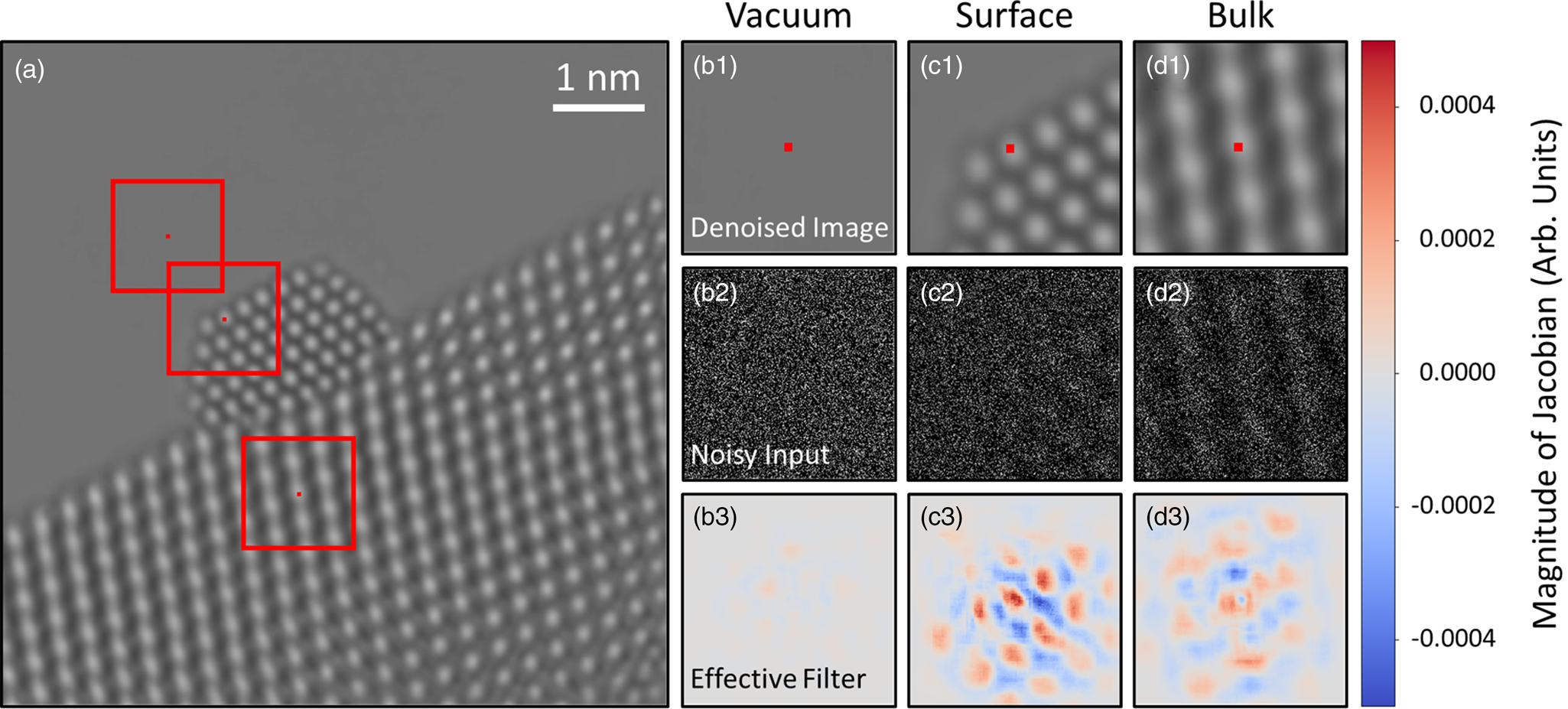
Fig. 8. Investigating the mechanism by which the network denoises experimental data. A denoised experimental image is shown in (a). Three regions of the image in the vacuum, catalyst surface, and bulk have been highlighted by red boxes and are depicted in (b1), (c1), and (d1), respectively. The central pixel in each windowed region is marked with a small red square. The noisy input within the network's receptive field around each pixel is displayed in (b2), (c2), and (d2). In (b3), (c3), and (d3), the Jacobian of the network at each pixel is plotted, which provides an interpretable visualization of the regions of the noisy input that have the most impact on the denoised estimate.
Interestingly, the effective filter shows considerable variation at different locations in the image. For the pixel in the vacuum, Figure 8b3 shows the gradient at this location is mostly uniform with a magnitude close to 0.0. The largely uniform gradient suggests the network senses a lack of structure in the vacuum and has incorporated this information into its denoising strategy. Compare this with the gradient plotted in Figure 8d3 for the pixel on an atomic column in the CeO2 bulk. Here, the gradient shows a clear periodicity, with a symmetric pattern that mirrors the local structure of the bulk material. The symmetry reveals that the network has learned to recognize an uninterrupted continuation of structure at this location. Note that the magnitude of the gradient in the region around the central pixel is comparable to that of the surrounding atomic column-like regions. The mostly equal weighting of local and nonlocal periodic information implies that the network considers the central atomic column to be similar to those surrounding it.
The network's denoising strategy adapts in response to nonperiodic structural features at the Pt nanoparticle surface. As seen in Figure 8c3, at the surface, the network gives substantially more weight to information that is in the immediate proximity of the pixel to be denoised. Strongly weighting the intensity within an atomic column-sized region may be what enables the network to recover the nonperiodic atomic features at the catalyst surface. In unfavorable cases, the same strategy could lead to artifacts if the noisy input contains a randomly bright clustering of intensity that resembles an atomic column. As in the CeO2 bulk, periodicity is seen in the gradient at the Pt surface, although now the separation distance between the atomic column-like regions has changed to match the periodicity of the projected Pt lattice. Notably, the spatial distribution of the filter is also now less symmetric, with the magnitude of the gradient diminishing to zero more rapidly in the regions that contain vacuum. Hence, the asymmetry reflects the termination of the nanoparticle structure and suggests that the network has learned to identify the presence of the catalyst surface.
Conclusion
A supervised deep CNN has been developed to denoise ultra-low SNR atomic-resolution TEM images of nanoparticles acquired during applications wherein the image signal is severely limited by Poisson shot noise. In this work, we have focused on data acquired on a direct detector operated in electron counting mode; however, in principle, the proposed network can be applied to data acquired in any mode, so long as the noise content can be modeled. Multislice image simulations were leveraged to generate a large dataset image for training and testing the network. The proposed network outperforms existing methods, including other CNNs, by a PSNR of 12.0 dB, achieving a PSNR of about 43 dB on a test set of simulated images (the typical starting PSNR of the data explored in this work is only 3 dB). We show that the network is generally robust to ±5 nm variations in defocus, although we suggest training the network using images at a defocus similar to the data that are to be denoised. The network's ability to correctly predict the atomic-scale structure of the nanoparticle surface was assessed by comparing the atomic columns originally present in clean simulations against those that appear in denoised images. We have also developed an approach based on the log-likelihood ratio test that provides a quantitative measure of the agreement between the noisy observation and the atomic-level structure present in the denoised image. The proposed assessment method requires only the network-denoised image and the noisy input and is therefore extensible to real experimental data, where no ground truth reference images exist. The network was applied to an experimentally acquired TEM image dataset of a CeO2-supported Pt nanoparticle. We have conducted a gradient-based analysis to investigate the mechanisms used by the network to denoise experimental images. Here, this shows the network both (a) exploits information on the surrounding structure and (b) adapts its filtering approach when it encounters nonperiodic terminations or atomic-level defects at the nanoparticle surface. The approaches described here may be applicable to a wide range of imaging applications that are characterized by ultra-low SNR, including the investigation of dynamic processes with time-resolved in situ microscopy or the study of beam-sensitive systems.
Supplementary material
To view supplementary material for this article, please visit https://doi.org/10.1017/S1431927621012678.
Acknowledgments
The authors gratefully acknowledge financial support from the National Science Foundation (NSF). NSF CBET Award 1604971 supported J.L.V. and P.A.C. NSF OAC Award 1940263 supported R.M. and P.A.C. NSF NRT HDR Award 1922658 partially supported S.M. NSF OAC Award 1940124 and NSF CCF Award 1934985 supported B.T. and D.S.M. NSF OAC Award 1940097 supported C.F.-G. The authors acknowledge HPC resources available through ASU, NYU, and Cornell, as well as the John M. Cowley Center for High Resolution Electron Microscopy at Arizona State University. The authors also gratefully acknowledge the use of microscopy resources at the National Institute of Standards and Technology in Gaithersburg, MD, and, in particular, the helpful assistance and hospitality of Dr. Wei-Chang David Yang, Dr. Canhui Wang, and Dr. Renu Sharma.
Author contributions statement
J.L.V. and P.A.C. acquired and processed the experimental data. R.M. and P.A.C. created the training dataset. S.M. designed, implemented, and analyzed the convolutional neural network and denoising methodology. B.T. contributed to implement the methodology and conducted the experiments, and D.M. supervised the design of the methodology. C.F.-G. supervised the design, implementation, and analysis of the methodology. D.Y.S. assisted with the implementation of the methodology; E.P.S. supervised the design, implementation, and analysis of the methodology.
Competing interests
The authors declare no competing interests.


 Open access