


1. Introduction
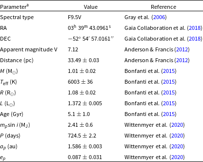
The detection of HD 23079b, reported by Tinney et al. (Reference Tinney, Butler, Marcy, Jones, Penny, McCarthy and Carter2002), was a successful outcome of the Anglo-Australian Planet Search. HD 23079b, a Jupiter-type planet, is hosted by a solar-type star with a temperature of about 6 000 K (Bonfanti et al. Reference Bonfanti, Ortolani, Piotto and Nascimbeni2015); see Table 1 for details. This system is located in the Southern sky in the constellation Reticulum. HD 23079b is in a nearly circular orbit situated at the outskirts of the stellar habitable zone (HZ) that extends between 0.87 and 2.03 au (optimistic limits; see Kopparapu et al. Reference Kopparapu2013, Reference Kipping and Teachey2014).
Stellar and planetary parameters.
a All parameters and symbols have their customary meaning.
The relatively low level of stellar activity of HD 23079, consistent with its age of $\sim$
5 Gyr (see Section 2.1), tends to favour the existence of a habitable circumstellar environment; see, e.g., Ribas et al. (Reference Ribas, Guinan, Güdel and Audard2005), Lammer et al. (Reference Lammer2009), Ramirez (Reference Ramirez2018) for more general discussions. However, massive planets such as HD 23079b with orbits located within stellar HZ tend to thwart the existence of habitable terrestrial planets owing to the onset of orbital instabilities (e.g., Jones, Sleep, & Chambers Reference Jones, Sleep and Chambers2001; Noble, Musielak, & Cuntz Reference Noble, Musielak and Cuntz2002; (e.g., Jones, Sleep, & Chambers Reference Jones, Sleep and Chambers2001; Noble, Musielak, & Cuntz Reference Noble, Musielak and Cuntz2002; Agnew et al. Reference Agnew, Maddison, Thilliez and Horner2017, Reference Saha and Tremaine2018). Nevertheless, there is a significant possibility for the existence of habitable Trojan planets and/or habitable exomoons (in orbit about HD 23079b), as demonstrated via detailed simulations; see Eberle et al. (Reference Eberle, Cuntz, Quarles and Musielak2011) and Cuntz et al. (Reference Cuntz, Quarles, Eberle and Shukayr2013), respectively.
$\sim$
5 Gyr (see Section 2.1), tends to favour the existence of a habitable circumstellar environment; see, e.g., Ribas et al. (Reference Ribas, Guinan, Güdel and Audard2005), Lammer et al. (Reference Lammer2009), Ramirez (Reference Ramirez2018) for more general discussions. However, massive planets such as HD 23079b with orbits located within stellar HZ tend to thwart the existence of habitable terrestrial planets owing to the onset of orbital instabilities (e.g., Jones, Sleep, & Chambers Reference Jones, Sleep and Chambers2001; Noble, Musielak, & Cuntz Reference Noble, Musielak and Cuntz2002; (e.g., Jones, Sleep, & Chambers Reference Jones, Sleep and Chambers2001; Noble, Musielak, & Cuntz Reference Noble, Musielak and Cuntz2002; Agnew et al. Reference Agnew, Maddison, Thilliez and Horner2017, Reference Saha and Tremaine2018). Nevertheless, there is a significant possibility for the existence of habitable Trojan planets and/or habitable exomoons (in orbit about HD 23079b), as demonstrated via detailed simulations; see Eberle et al. (Reference Eberle, Cuntz, Quarles and Musielak2011) and Cuntz et al. (Reference Cuntz, Quarles, Eberle and Shukayr2013), respectively.
The search for exomoons has been an active endeavour after the launch of the Kepler Space Telescope, while many works (Sartoretti & Schneider Reference Sartoretti and Schneider1999; Cabrera & Schneider Reference Cabrera and Schneider2007; Kipping Reference Kipping2009a, Reference Idini and Stevensonb) preceding the Kepler era laid the theoretical groundwork for their detection through transit timing and duration variations. However, such methods have limitations (Kipping & Teachey Reference Kipping and Teachey2020; Kipping Reference Kipping2021) and photometric observations can still lead to false positives, including one candidate for Kepler-90g (Kipping et al. Reference Kipping, Huang, Nesvorný, Torres, Buchhave, Bakos and Schmitt2015a).
Fortunately, there are other methods proposed for exomoon detection including using a planet profile determined by the average light curve (Simon et al. Reference Simon, Szabó, Kiss and SzatmÁry2012), optimising with respect to the orbital sampling effect (Heller Reference Heller2014; Heller, Hippke, & Jackson Reference Heller, Hippke and Jackson2016; Hippke Reference Hippke2015), Doppler monitoring of directly imaged exoplanets (Agol et al. Reference Agol, Jansen, Lacy, Robinson and Meadows2015; Vanderburg, Rappaport, & Mayo Reference Vanderburg, Rappaport and Mayo2018) or examining the radio emissions from giant exoplanets (Noyola, Satyal, & Musielak Reference Noyola, Satyal and Musielak2014, Reference Kopparapu and Ramirez2016). Another motivation for our study stems from the recent discovery of a circumplanetary disk (system PDS 70), indicating the ongoing formation of one or more exomoons in alignment with the Hill radius criterion (Benisty et al. Reference Benisty2021).
Theoretical constraints aid in the interpretation of observations and can be useful to quickly validate whether a exomoon candidate is plausible or not (Quarles, Li, & Rosario-Franco Reference Rosario-Franco, Quarles, Musielak and Cuntz2020b). One of these constraints is the combined tidal interaction between the host star, planet and moon (Barnes & O’Brien Reference Barnes and O’Brien2002; Sasaki, Barnes, & O’Brien Reference Sasaki, Barnes and O’Brien2012; Sasaki & Barnes Reference Sasaki and Barnes2014; Lainey et al. Reference Lainey2020) that generally depends on a wide range of parameters (e.g., tidal Love number and tidal quality factor). Spalding, Batygin, & Adams (Reference Spalding, Batygin and Adams2016) explored how the so-called ‘evection resonance’ can cause significant growth in a moon’s eccentricity, which can lead to the moon’s tidal breakup or escape from the planet’s gravitational influence.
Nearby (Payne et al. Reference Payne, Deck, Holman and Perets2013) and distant planetary companions (Grishin et al. Reference Grishin, Perets, Zenati and Michaely2017) can also drive an exomoon along a similar path to destruction. Even without these confounding interactions, Domingos, Winter, & Yokoyama (Reference Domingos, Winter and Yokoyama2006) produced estimates for exomoon stability using three-body interactions, but these results represent the upper boundary of a transition region for stability (Dvorak Reference Dvorak1986). Recently, Rosario-Franco et al. (Reference Rosario-Franco, Quarles, Musielak and Cuntz2020) determined a revised fitting formula for the (more conservative) lower stability boundary for prograde satellites, whereas Quarles et al. (Reference Quarles, Eggl, Rosario-Franco and Li2021) derived a similar fitting formula for retrograde satellites.
In this study, we revisit the existence of possible exomoons in the HD 23079 system based on more generalised assumptions and an improved methodology. Our paper is structured as follows. In Section 2, we summarize our theoretical approach. Our results and discussion are conveyed in Section 3 including comparisons to previous works. Here we also comment on the observability of possible HD 23079 exomoons. In Section 4, we report our summary and conclusions.
2. Theoretical approach
2.1. Stellar and planetary parameters
HD 23079 is a solar-type star of spectral type F9.5V (Gray et al. Reference Gray, Corbally, Garrison, McFadden, Bubar, McGahee, O’Donoghue and Knox2006) with an effective temperature of about 6 003 K (Bonfanti et al. Reference Bonfanti, Ortolani, Piotto and Nascimbeni2015); see Table 1. Its mass and radius are given as $1.01 \pm 0.02$
M
$1.01 \pm 0.02$
M $_\odot$
and
$_\odot$
and $1.08 \pm 0.02$
R
$1.08 \pm 0.02$
R $_\odot$
, respectively. HD 23079 has an age of approximately 5 Gyr (Saffe, Gómez, & Chavero Reference Saffe, Gómez and Chavero2005; Bonfanti et al. Reference Bonfanti, Ortolani, Piotto and Nascimbeni2015), which implies a relatively low level of chromospheric activity—a notable feature in support of circumstellar habitability (e.g., Kasting & Catling Reference Kasting and Catling2003; Lammer et al. Reference Lammer2009; Kaltenegger Reference Kaltenegger2017). The minimum mass
$_\odot$
, respectively. HD 23079 has an age of approximately 5 Gyr (Saffe, Gómez, & Chavero Reference Saffe, Gómez and Chavero2005; Bonfanti et al. Reference Bonfanti, Ortolani, Piotto and Nascimbeni2015), which implies a relatively low level of chromospheric activity—a notable feature in support of circumstellar habitability (e.g., Kasting & Catling Reference Kasting and Catling2003; Lammer et al. Reference Lammer2009; Kaltenegger Reference Kaltenegger2017). The minimum mass $m_{p}{\sin}i$
of the planet HD 23079b, discovered by Tinney et al. (Reference Tinney, Butler, Marcy, Jones, Penny, McCarthy and Carter2002), has been identified as
$m_{p}{\sin}i$
of the planet HD 23079b, discovered by Tinney et al. (Reference Tinney, Butler, Marcy, Jones, Penny, McCarthy and Carter2002), has been identified as $2.41 \pm 0.6$
M
$2.41 \pm 0.6$
M $_{\rm J}$
; however, the exact value of
$_{\rm J}$
; however, the exact value of $m_{p}$
is unknown owing to the inherent limitations of the radial velocity (RV) method.
$m_{p}$
is unknown owing to the inherent limitations of the radial velocity (RV) method.
The stellar luminosity is about 35% larger than that of the Sun; hence, the HZ of HD 23079 is notably wider and further extended than the Solar HZ. In fact, the outer limits of the conservative and optimistic HZ are identified as 1.93 and 2.03 au, respectively. The orbital parameters of the planet, i.e., the semimajor axis $a_{p}$
and the eccentricity
$a_{p}$
and the eccentricity $e_{p}$
, are given as 1.586
$e_{p}$
, are given as 1.586 $\pm$
0.003 au and 0.087
$\pm$
0.003 au and 0.087 $\pm$
0.031, respectively, indicating that HD 23079b is situated in a nearly circular orbit within the stellar HZ at an orbital distance akin to that of Mars relative to the Sun. The planetary Hill radius is given as:
$\pm$
0.031, respectively, indicating that HD 23079b is situated in a nearly circular orbit within the stellar HZ at an orbital distance akin to that of Mars relative to the Sun. The planetary Hill radius is given as:
 \begin{equation} R_{\rm H} = a_{p}\left(\frac{m_{p}+m_{\rm sat}}{3M_\star}\right)^{1/3},\end{equation}
which includes the planet, satellite and stellar mass ( $m_{p}$
,
$m_{p}$
, $m_{\rm sat}$
, and
$m_{\rm sat}$
, and $M_\star$
, respectively) in addition to the planetary semimajor axis
$M_\star$
, respectively) in addition to the planetary semimajor axis $a_{p}$
. In physical units, the Hill radius is approximately 0.144 au using the appropriate values from Table 1. This formulation of the Hill radius is appropriate because the planetary eccentricity is low and no significant third body exists that can substantially force the planetary eccentricity (Quarles et al. Reference Quarles, Eggl, Rosario-Franco and Li2021).
$a_{p}$
. In physical units, the Hill radius is approximately 0.144 au using the appropriate values from Table 1. This formulation of the Hill radius is appropriate because the planetary eccentricity is low and no significant third body exists that can substantially force the planetary eccentricity (Quarles et al. Reference Quarles, Eggl, Rosario-Franco and Li2021).
2.2. N-body simulations
To investigate the potential for exomoons in HD 23079, we perform a series of numerical simulations that identify the orbital stability of an Earth-mass satellite orbiting HD 23079b, a Jupiter-like planet. The numerical simulations are carried out using the general N-body software REBOUND (Rein & Liu Reference Rein and Liu2012) with its IAS15 adaptive step integration scheme (Rein & Spiegel Reference Rein and Spiegel2015). The IAS15 integrator is necessary because our study explores both prograde ( $i_{\rm sat} = 0^\circ$
) and retrograde (
$i_{\rm sat} = 0^\circ$
) and retrograde ( $i_{\rm sat} = 180^\circ$
) satellite orbits, where the latter can be highly eccentric. Adaptive step integrators, although more accurate, can also be more computationally expensive.
$i_{\rm sat} = 180^\circ$
) satellite orbits, where the latter can be highly eccentric. Adaptive step integrators, although more accurate, can also be more computationally expensive.
We set the initial timestep equal to 5% of the shortest satellite orbital period ( $\sim$
0.007 yr for prograde or
$\sim$
0.007 yr for prograde or $\sim$
0.017 yr for retrograde) and define 0.0001 yr as the minimum allowed timestep with the default accuracy parameter
$\sim$
0.017 yr for retrograde) and define 0.0001 yr as the minimum allowed timestep with the default accuracy parameter $10^{-9}$
used for the IAS15 integrator. Cuntz et al. (Reference Cuntz, Quarles, Eberle and Shukayr2013) showed that the outcomes of simulations are identical for timesteps smaller than the prescribed minimum using other adaptive timestep methods. The simulation timescale of our N-body integrations is
$10^{-9}$
used for the IAS15 integrator. Cuntz et al. (Reference Cuntz, Quarles, Eberle and Shukayr2013) showed that the outcomes of simulations are identical for timesteps smaller than the prescribed minimum using other adaptive timestep methods. The simulation timescale of our N-body integrations is $10^5$
years, which is typical for determining the stability limits for hierarchical systems within large parameter spaces (Rosario-Franco et al. Reference Rosario-Franco, Quarles, Musielak and Cuntz2020; Quarles et al. Reference Quarles, Li, Kostov and Haghighipour2020a; Quarles et al. Reference Quarles, Eggl, Rosario-Franco and Li2021).
$10^5$
years, which is typical for determining the stability limits for hierarchical systems within large parameter spaces (Rosario-Franco et al. Reference Rosario-Franco, Quarles, Musielak and Cuntz2020; Quarles et al. Reference Quarles, Li, Kostov and Haghighipour2020a; Quarles et al. Reference Quarles, Eggl, Rosario-Franco and Li2021).
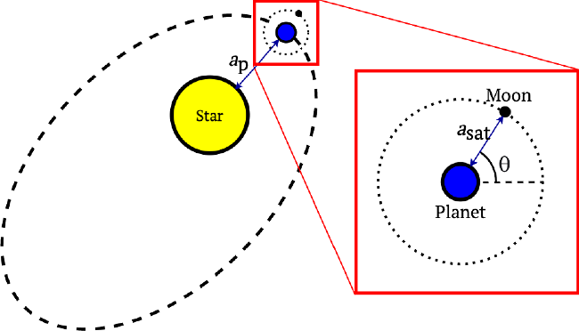
Each simulation begins centered around the host star, HD 23079, with the host planet and satellite added hierarchically using a Jacobi coordinate system (see Figure 1). The planet begins at its periastron position $\omega_{p}$
and the line of apsides
$\omega_{p}$
and the line of apsides $\Omega_{p}$
is used as the reference direction (
$\Omega_{p}$
is used as the reference direction ( $\omega_{p} = \Omega_{p} = 0^\circ$
). An initial condition is classified as potentially stable if the satellite does not encounter either of our stopping criteria to detect instabilities. We stop our simulations and classify an initial condition as unstable if the putative satellite: (a) crosses the planet’s Hill radius thereby leaving the region over which the planet’s gravitational influence dominates over that of the star or (b) collides with the host planet over a given timescale. In addition, we require that a stable initial condition does not depend on the initial mean anomaly
$\omega_{p} = \Omega_{p} = 0^\circ$
). An initial condition is classified as potentially stable if the satellite does not encounter either of our stopping criteria to detect instabilities. We stop our simulations and classify an initial condition as unstable if the putative satellite: (a) crosses the planet’s Hill radius thereby leaving the region over which the planet’s gravitational influence dominates over that of the star or (b) collides with the host planet over a given timescale. In addition, we require that a stable initial condition does not depend on the initial mean anomaly $\theta$
of the satellite (Figure 1), which largely excludes islands of quasi-stability due to MMRs (Mudryk & Wu Reference Mudryk and Wu2006).
$\theta$
of the satellite (Figure 1), which largely excludes islands of quasi-stability due to MMRs (Mudryk & Wu Reference Mudryk and Wu2006).
Representation of the initial conditions of the HD 23079 system in our calculations: (a) Planet HD 23079b (blue dot) orbits star HD 23079 (yellow dot). (b) An exomoon (black dot) orbits HD 23079b. Initially, the planet HD 23079b starts at perihelion and the exomoon starts at a random angle ( $\theta$
) with respect to the planet for each simulation.
$\theta$
) with respect to the planet for each simulation.
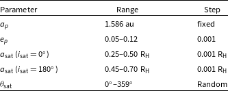
Cuntz et al. (Reference Cuntz, Quarles, Eberle and Shukayr2013) explored a parameter space that varied the initial planetary semimajor axis, eccentricity and the satellite’s semimajor axis $a_{\rm sat}$
. Recent observations (Wittenmyer et al. Reference Wittenmyer2020) greatly narrowed the uncertainty of the planetary semimajor axis; therefore, we keep the planetary semimajor axis fixed (
$a_{\rm sat}$
. Recent observations (Wittenmyer et al. Reference Wittenmyer2020) greatly narrowed the uncertainty of the planetary semimajor axis; therefore, we keep the planetary semimajor axis fixed ( $a_{p} = 1.586$
au) throughout this work. However, we evaluate simulations varying the planetary eccentricity
$a_{p} = 1.586$
au) throughout this work. However, we evaluate simulations varying the planetary eccentricity $e_{\rm sat}$
from 0.05 to 0.12 in 0.001 steps motivated by the observational uncertainties. The prograde simulations are evaluated using a satellite semimajor axis from 0.25 to 0.5 R
$e_{\rm sat}$
from 0.05 to 0.12 in 0.001 steps motivated by the observational uncertainties. The prograde simulations are evaluated using a satellite semimajor axis from 0.25 to 0.5 R $_{\rm H}$
in steps of 0.001 R
$_{\rm H}$
in steps of 0.001 R $_{\rm H}$
, where R
$_{\rm H}$
, where R $_{\rm H}$
is the planet’s Hill radius and the range in R
$_{\rm H}$
is the planet’s Hill radius and the range in R $_{\rm H}$
is motivated by previous observational and dynamical studies of satellites (Cruikshank et al. Reference Cruikshank, Degewij and Zellner1982; Saha & Tremaine Reference Saha and Tremaine1993; Domingos et al. Reference Domingos, Winter and Yokoyama2006; Jewitt & Haghighipour Reference Jewitt and Haghighipour2007; Donnison Reference Donnison2010; Rosario-Franco et al. Reference Rosario-Franco, Quarles, Musielak and Cuntz2020; Quarles et al. Reference Quarles, Eggl, Rosario-Franco and Li2021). Many studies (Henon Reference Henon1970; Hamilton & Burns Reference Hamilton and Burns1991; Morais & Giuppone 2012; Grishin et al. Reference Grishin, Perets, Zenati and Michaely2017; Quarles et al. Reference Quarles, Eggl, Rosario-Franco and Li2021) have demonstrated that retrograde orbital stability extends to larger values of the satellite semimajor axis compared to the prograde case. Thus, we increased the
$_{\rm H}$
is motivated by previous observational and dynamical studies of satellites (Cruikshank et al. Reference Cruikshank, Degewij and Zellner1982; Saha & Tremaine Reference Saha and Tremaine1993; Domingos et al. Reference Domingos, Winter and Yokoyama2006; Jewitt & Haghighipour Reference Jewitt and Haghighipour2007; Donnison Reference Donnison2010; Rosario-Franco et al. Reference Rosario-Franco, Quarles, Musielak and Cuntz2020; Quarles et al. Reference Quarles, Eggl, Rosario-Franco and Li2021). Many studies (Henon Reference Henon1970; Hamilton & Burns Reference Hamilton and Burns1991; Morais & Giuppone 2012; Grishin et al. Reference Grishin, Perets, Zenati and Michaely2017; Quarles et al. Reference Quarles, Eggl, Rosario-Franco and Li2021) have demonstrated that retrograde orbital stability extends to larger values of the satellite semimajor axis compared to the prograde case. Thus, we increased the $a_{\rm sat}$
range to 0.45–0.70 R
$a_{\rm sat}$
range to 0.45–0.70 R $_{\rm H}$
with a 0.001 R
$_{\rm H}$
with a 0.001 R $_{\rm H}$
step size. In physical units, a 0.001 R
$_{\rm H}$
step size. In physical units, a 0.001 R $_{\rm H}$
step corresponds to approximately 0.0001 au, noting that we scale the steps with respect to the Hill radius as this approach will allow our results to scale with improved characterisations of the planetary and stellar parameters, if available. The parameter ranges for our N-body simulations are summarized in Table 2.
$_{\rm H}$
step corresponds to approximately 0.0001 au, noting that we scale the steps with respect to the Hill radius as this approach will allow our results to scale with improved characterisations of the planetary and stellar parameters, if available. The parameter ranges for our N-body simulations are summarized in Table 2.
N-body simulation parameters.
In each simulation, the moon begins on a circular orbit that is apsidally aligned ( $\omega_{\rm sat}=\Omega_{\rm sat}=0^\circ$
) with the planetary orbit. For each combination of planetary eccentricity and the satellite’s semimajor axis, 20 simulations are evolved using a random mean anomaly
$\omega_{\rm sat}=\Omega_{\rm sat}=0^\circ$
) with the planetary orbit. For each combination of planetary eccentricity and the satellite’s semimajor axis, 20 simulations are evolved using a random mean anomaly $\theta$
for the satellite chosen from 0
$\theta$
for the satellite chosen from 0 $^\circ$
–
$^\circ$
– $359^\circ$
. We use a parameter
$359^\circ$
. We use a parameter $f_{\rm stab}$
to summarize these trials, which represents the fraction of stable simulations for a given (
$f_{\rm stab}$
to summarize these trials, which represents the fraction of stable simulations for a given ( $e_{p}, a_{\rm sat}$
) combination.
$e_{p}, a_{\rm sat}$
) combination.
2.3. Satellite orbital migration due to tides
A satellite’s long-term evolution is affected by tides raised on its host planet, where the induced tidal bulge slows the planet’s rotation over billion-year timescales. Through the conservation of angular momentum, the satellite can fall toward the planet or migrate outward toward the Hill radius. The satellite’s migration depends on whether its orbital period $T_{\rm sat}$
is greater than (outward migration) or less than (inward migration) the host planet’s rotation period
$T_{\rm sat}$
is greater than (outward migration) or less than (inward migration) the host planet’s rotation period $P_{\rm rot}$
. We begin the satellite on a circular, coplanar orbit relative to the Roche radius (
$P_{\rm rot}$
. We begin the satellite on a circular, coplanar orbit relative to the Roche radius ( $a_{\rm sat}=3R_{\rm roche}$
) with the satellite treated as a fluid satellite, and Roche radius calculated via:
$a_{\rm sat}=3R_{\rm roche}$
) with the satellite treated as a fluid satellite, and Roche radius calculated via:
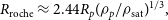 \begin{equation} R_{\rm roche} \approx 2.44 R_{p}(\rho_{p}/\rho_{\rm sat})^{1/3},\end{equation}
where the planet radius $R_{p}$
is assumed to equal the radius of Jupiter given the well-established trends in the mass radius relation for giant planets (Fortney et al. Reference Fortney, Marley and Barnes2007; Chen & Kipping Reference Chen and Kipping2017), the planet density
$R_{p}$
is assumed to equal the radius of Jupiter given the well-established trends in the mass radius relation for giant planets (Fortney et al. Reference Fortney, Marley and Barnes2007; Chen & Kipping Reference Chen and Kipping2017), the planet density $\rho_{p}$
is 1.33 g cm–3 (Jupiter-like), and the satellite density is 5.515 g cm–3 (Earth-like). A satellite at 3
$\rho_{p}$
is 1.33 g cm–3 (Jupiter-like), and the satellite density is 5.515 g cm–3 (Earth-like). A satellite at 3 $\times$
the Roche radius begins an orbital period of
$\times$
the Roche radius begins an orbital period of $\sim$
18 h. From theoretical calculations and numerical simulations of giant planet formation (Takata & Stevenson Reference Takata and Stevenson1996; Batygin Reference Batygin2018), giant planets are expected to be rapid rotators (
$\sim$
18 h. From theoretical calculations and numerical simulations of giant planet formation (Takata & Stevenson Reference Takata and Stevenson1996; Batygin Reference Batygin2018), giant planets are expected to be rapid rotators ( $\sim$
3 h) due to gas accretion or rotate more slowly (
$\sim$
3 h) due to gas accretion or rotate more slowly ( $\sim$
10–12 h) like the Solar System giant planets if magnetic braking is efficient. Since the satellite’s orbital period (
$\sim$
10–12 h) like the Solar System giant planets if magnetic braking is efficient. Since the satellite’s orbital period ( $\sim$
18 h at
$\sim$
18 h at $3 R_{\rm roche}$
) is greater than the expected spin period of giant planets, the satellite will undergo outward migration.
$3 R_{\rm roche}$
) is greater than the expected spin period of giant planets, the satellite will undergo outward migration.
Equilibrium tidal models are commonly prescribed within two types: constant phase lag (CPL; Goldreich & Soter Reference Goldreich and Soter1966) or constant time lag (CTL; Hut Reference Hut1981). Both models require an assumption for the Love number $k_2$
(Love Reference Love1911) and a moment of inertia factor
$k_2$
(Love Reference Love1911) and a moment of inertia factor $\alpha$
, for which we use Jupiter-like values (0.565 and 0.2756, respectively) determined from the Juno probe (Ni Reference Ni2018; Idini & Stevenson Reference Idini and Stevenson2021). The tidal models differ in their approach to approximating the tidal dissipation
$\alpha$
, for which we use Jupiter-like values (0.565 and 0.2756, respectively) determined from the Juno probe (Ni Reference Ni2018; Idini & Stevenson Reference Idini and Stevenson2021). The tidal models differ in their approach to approximating the tidal dissipation $\epsilon$
, where the CPL model implements a constant Q and the CTL model uses a constant timelag
$\epsilon$
, where the CPL model implements a constant Q and the CTL model uses a constant timelag $\tau$
.
$\tau$
.
Both models yield similar results for small satellite-planet mass ratios, but the CTL model more accurately represents the tidal forcing frequencies (Ogilvie Reference Ogilvie2014); thus, we use a CTL model. The constant timelag $\tau$
is unknown for HD 23079b; hence, we assume a Jupiter-like value (
$\tau$
is unknown for HD 23079b; hence, we assume a Jupiter-like value ( $\tau_{\rm J}\sim 0.035$
s) while evaluating models over several orders of magnitude (
$\tau_{\rm J}\sim 0.035$
s) while evaluating models over several orders of magnitude ( $10^{-2}-10^2\;\tau_{\rm J}$
). The planetary mass given in Table 1 is determined through the RV method, which allows an observer to determine the minimum mass
$10^{-2}-10^2\;\tau_{\rm J}$
). The planetary mass given in Table 1 is determined through the RV method, which allows an observer to determine the minimum mass $m_{p}$
. Therefore, we evolve the tidal model considering three host planet masses (1, 1.5 and 2
$m_{p}$
. Therefore, we evolve the tidal model considering three host planet masses (1, 1.5 and 2 $m_{p}$
) with a Jupiter-like
$m_{p}$
) with a Jupiter-like $\tau$
. Herein we use the CTL model derived by Hut (Reference Hut1981) assuming zero planetary obliquity, which is equivalent to the formalism described in more recent approaches (Leconte et al. Reference Leconte, Chabrier, Baraffe and Levrard2010; Heller, Leconte, & Barnes Reference Heller, Leconte and Barnes2011; Barnes Reference Barnes2017).
$\tau$
. Herein we use the CTL model derived by Hut (Reference Hut1981) assuming zero planetary obliquity, which is equivalent to the formalism described in more recent approaches (Leconte et al. Reference Leconte, Chabrier, Baraffe and Levrard2010; Heller, Leconte, & Barnes Reference Heller, Leconte and Barnes2011; Barnes Reference Barnes2017).
The tidal evolution with respect to time t is described by the following equations:
 \begin{align}\frac{da_i}{dt} &= \frac{2a_i^2 Z_{{p},j}}{G m_{p} m_j} \left(\frac{f_2(e_i)}{\beta^{12}(e_i)} \frac{\Omega_{p}}{n_j} - \frac{f_1(e_i)}{\beta^{15}(e_i)} \right),\qquad \end{align}
 \begin{align}\frac{de_i}{dt} &= \frac{11a_ie_i Z_{{p},j}}{2G m_{p} m_j} \left(\frac{f_4(e_i)}{\beta^{12}(e_i)} \frac{\Omega_{p}}{n_j} - \frac{18}{11}\frac{f_3(e_i)}{\beta^{13}(e_i)} \right), \end{align}
and
 \begin{align} \frac{d\Omega_{p}}{dt} = \sum_j \frac{Z_{{p},j}}{2 \alpha_{p} m_{p} R^2_{p} n_j} \left(\frac{2 f_2(e_j)}{\beta^{12}(e_j)} - \frac{f_5(e_j)}{\beta^9(e_j)} \frac{\Omega_{p}}{n_j}\right),\end{align}
where
 \begin{equation}Z_{{p},j} \equiv 3G^2k_{2,p}\tau_{p} m^2_j ( m_{p} + m_j ) \frac{R_{p}^5}{a_i^9}\end{equation}
and
 \begin{equation} \begin{aligned} \beta(e) &= \sqrt{1 - e^2}, \\[3pt] f_1(e) &= 1 + \frac{31}{2}e^2 + \frac{255}{8}e^4 + \frac{185}{16}e^6 + \frac{25}{64}e^8, \\[3pt] f_2(e) &= 1 + \frac{15}{2}e^2 + \frac{45}{8}e^4 + \frac{5}{16}e^6 \\[3pt] f_3(e) &= 1 + \frac{15}{4}e^2 + \frac{15}{8}e^4 + \frac{5}{64}e^6, \\[3pt] f_4(e) &= 1 + \frac{3}{2}e^2 + \frac{1}{8}e^4,\\[3pt] f_5(e) &= 1 + 3e^2 + \frac{3}{8}e^4.\end{aligned}\end{equation}
Equations (3) and (4) describe the semimajor axis and eccentricity evolution of either the planet or satellite through the subscript i. The subscript j represents either the host star or the satellite that is raising the tide on the planet, where $n_j$
is the respective orbital mean motion. Equation (5) describes the spin evolution of the planet, where the moon is assumed to be synchronously rotating and the changes to the host star’s spin are negligible. The subscript j in Equation (5) represents either the host star or the satellite that is contributing to spin-down the planet. A Jupiter-like value is used for the moment of inertia factor (
$n_j$
is the respective orbital mean motion. Equation (5) describes the spin evolution of the planet, where the moon is assumed to be synchronously rotating and the changes to the host star’s spin are negligible. The subscript j in Equation (5) represents either the host star or the satellite that is contributing to spin-down the planet. A Jupiter-like value is used for the moment of inertia factor ( $\alpha_{p}=0.565$
) and G represents the Newtonian constant of gravitation.
$\alpha_{p}=0.565$
) and G represents the Newtonian constant of gravitation.
3. Results and Discussion
3.1. Model simulations
Recent observations by Benisty et al. (Reference Benisty2021) revealed the existence of a circumplanetary disk around PDS 70c, a planet observed to be in the process of accreting gas. After this stage, more massive satellites could be acquired through processes of tidal capture and pull down (Hamers & Portegies Zwart Reference Hamers and Portegies Zwart2018) as has been suggested for the candidate exomoon Kepler 1625b-I (Teachey & Kipping Reference Teachey and Kipping2018). Assuming that exomoons form soon after the epoch of planet formation, such moons must survive against perturbations from the host star to be observed in the present day ( $\sim$
5 Gyr; Bonfanti et al. Reference Bonfanti, Ortolani, Piotto and Nascimbeni2015). Our goal is to determine the stability boundary of putative satellites around the host planet, HD 23079b. Previously, Eberle et al. (Reference Eberle, Cuntz, Quarles and Musielak2011) and Cuntz et al. (Reference Cuntz, Quarles, Eberle and Shukayr2013) discussed the orbital stability limit of an Earth-mass object in this system as a Trojan planet or a natural satellite within the planet’s Hill radius.
$\sim$
5 Gyr; Bonfanti et al. Reference Bonfanti, Ortolani, Piotto and Nascimbeni2015). Our goal is to determine the stability boundary of putative satellites around the host planet, HD 23079b. Previously, Eberle et al. (Reference Eberle, Cuntz, Quarles and Musielak2011) and Cuntz et al. (Reference Cuntz, Quarles, Eberle and Shukayr2013) discussed the orbital stability limit of an Earth-mass object in this system as a Trojan planet or a natural satellite within the planet’s Hill radius.
We examine the orbital stability limit for prograde and retrograde orbits using N-body simulations with REBOUND (see Section 2.2). These simulations consider a range of initial planetary eccentricity consistent with current observational constraints (Wittenmyer et al. Reference Wittenmyer2020). Rosario-Franco et al. (Reference Rosario-Franco, Quarles, Musielak and Cuntz2020) and Quarles et al. (Reference Quarles, Eggl, Rosario-Franco and Li2021) provided rough estimates for the stability limit in terms of the planet’s Hill radius, whereas here we explore this system in much finer detail. Similar to Rosario-Franco et al. (Reference Rosario-Franco, Quarles, Musielak and Cuntz2020) and Quarles et al. (Reference Quarles, Eggl, Rosario-Franco and Li2021), we use the lower critical orbit (Rabl & Dvorak Reference Rabl and Dvorak1988) to define the stability limit, which is a more conservative approach that excludes regions of quasi-stability.
Figure 2 demonstrates the results of our simulations in terms of initial semimajor axis of the satellite $a_{\rm sat}$
(in R
$a_{\rm sat}$
(in R $_{\rm H}$
) and the planetary eccentricity
$_{\rm H}$
) and the planetary eccentricity $e_{p}$
. Figure 2a and b are colour-coded using the parameter
$e_{p}$
. Figure 2a and b are colour-coded using the parameter $f_{\rm stab}$
, which is defined as the fraction of 20 simulations with random mean anomalies for the satellite that survive for
$f_{\rm stab}$
, which is defined as the fraction of 20 simulations with random mean anomalies for the satellite that survive for $10^5$
yr. The values of
$10^5$
yr. The values of $f_{\rm stab}$
range from 0.0 to 1.0, where the cells with
$f_{\rm stab}$
range from 0.0 to 1.0, where the cells with $f_{\rm stab}<0.05$
(wholly unstable) are colored white. The fully stable (
$f_{\rm stab}<0.05$
(wholly unstable) are colored white. The fully stable ( $f_{\rm stab}=1$
; black) cells are used in our calculation of the stability boundary, while the values between the extremes illustrate regions of quasi-stability. The dashed (cyan) curves mark the stability limit previously determined for prograde (Rosario-Franco et al. Reference Rosario-Franco, Quarles, Musielak and Cuntz2020) and retrograde (Quarles et al. Reference Quarles, Eggl, Rosario-Franco and Li2021) satellites, respectively.
$f_{\rm stab}=1$
; black) cells are used in our calculation of the stability boundary, while the values between the extremes illustrate regions of quasi-stability. The dashed (cyan) curves mark the stability limit previously determined for prograde (Rosario-Franco et al. Reference Rosario-Franco, Quarles, Musielak and Cuntz2020) and retrograde (Quarles et al. Reference Quarles, Eggl, Rosario-Franco and Li2021) satellites, respectively.
Numerical estimates for the stability of (a) prograde and (b) retrograde exomoons orbiting HD 23079b as a function of the satellite’s initial semimajor axis $a_{\rm sat}$
in units of the planetary Hill radius R
$a_{\rm sat}$
in units of the planetary Hill radius R $_{\rm H}$
and the planetary eccentricity
$_{\rm H}$
and the planetary eccentricity $e_{p}$
. The colour code represents the fraction
$e_{p}$
. The colour code represents the fraction $f_{\rm stab}$
(out of 20) of stable simulations for a
$f_{\rm stab}$
(out of 20) of stable simulations for a $10^5$
yr timescale; it shows which initial parameters depend on the initial placement of the satellite through its mean anomaly
$10^5$
yr timescale; it shows which initial parameters depend on the initial placement of the satellite through its mean anomaly $\theta_{\rm sat}$
. The white cells denote cases where zero trial simulations survive for
$\theta_{\rm sat}$
. The white cells denote cases where zero trial simulations survive for $10^5$
yr and, conversely, the black cells denote cases where all the trial simulations survive. The cyan (dashed) lines mark the expected stability limits for (a) prograde (Rosario-Franco et al. Reference Rosario-Franco, Quarles, Musielak and Cuntz2020) and (b) retrograde (Quarles et al. Reference Quarles, Eggl, Rosario-Franco and Li2021) orbiting exommons. The green stars in (a) mark the previous estimates from Cuntz et al. (Reference Cuntz, Quarles, Eberle and Shukayr2013), which are found to lie at the border of the quasi-stable regime.
$10^5$
yr and, conversely, the black cells denote cases where all the trial simulations survive. The cyan (dashed) lines mark the expected stability limits for (a) prograde (Rosario-Franco et al. Reference Rosario-Franco, Quarles, Musielak and Cuntz2020) and (b) retrograde (Quarles et al. Reference Quarles, Eggl, Rosario-Franco and Li2021) orbiting exommons. The green stars in (a) mark the previous estimates from Cuntz et al. (Reference Cuntz, Quarles, Eberle and Shukayr2013), which are found to lie at the border of the quasi-stable regime.
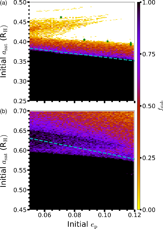
For prograde orbits (Figure 2a), the stability limit extends to 0.37 R $_{\rm H}$
for the lowest consider planet eccentricity and decreases to 0.35 R
$_{\rm H}$
for the lowest consider planet eccentricity and decreases to 0.35 R $_{\rm H}$
for larger planetary eccentricity. Our stability limit closely agrees with the stability fitting formula by Rosario-Franco et al. (Reference Rosario-Franco, Quarles, Musielak and Cuntz2020). Beyond this boundary, there is a gradient of quasi-stability over a small range in satellite semimajor axis. At
$_{\rm H}$
for larger planetary eccentricity. Our stability limit closely agrees with the stability fitting formula by Rosario-Franco et al. (Reference Rosario-Franco, Quarles, Musielak and Cuntz2020). Beyond this boundary, there is a gradient of quasi-stability over a small range in satellite semimajor axis. At $\sim$
0.43 R
$\sim$
0.43 R $_{\rm H}$
, there is a 6:1 (first-order) mean motion resonance (MMR) between the planet and satellite orbits (Quarles et al. Reference Quarles, Eggl, Rosario-Franco and Li2021). The MMR excites the satellite’s eccentricity over time, which allows for the satellite to escape as its apocenter extends beyond the upper critical orbit (
$_{\rm H}$
, there is a 6:1 (first-order) mean motion resonance (MMR) between the planet and satellite orbits (Quarles et al. Reference Quarles, Eggl, Rosario-Franco and Li2021). The MMR excites the satellite’s eccentricity over time, which allows for the satellite to escape as its apocenter extends beyond the upper critical orbit ( $\approx$
0.5 R
$\approx$
0.5 R $_{\rm H}$
; Domingos et al. Reference Domingos, Winter and Yokoyama2006). The MMR’s resonant angle depends on the relative orientation (i.e., mean anomaly) of the planetary and satellite orbits and particular starting angles can survive for longer periods, if the satellite returns to approximately the same phase after six orbits. Cuntz et al. (Reference Cuntz, Quarles, Eberle and Shukayr2013) used a single initial mean anomaly for the satellite, which largely corresponds to the upper critical orbit (green stars in Figure 2a).
$_{\rm H}$
; Domingos et al. Reference Domingos, Winter and Yokoyama2006). The MMR’s resonant angle depends on the relative orientation (i.e., mean anomaly) of the planetary and satellite orbits and particular starting angles can survive for longer periods, if the satellite returns to approximately the same phase after six orbits. Cuntz et al. (Reference Cuntz, Quarles, Eberle and Shukayr2013) used a single initial mean anomaly for the satellite, which largely corresponds to the upper critical orbit (green stars in Figure 2a).
For retrograde orbits (Figure 2b), the continuously stable region extends to $\sim$
0.59 R
$\sim$
0.59 R $_{\rm H}$
for
$_{\rm H}$
for $e_{p}$
= 0.05 and recedes to
$e_{p}$
= 0.05 and recedes to $\sim$
0.57 R
$\sim$
0.57 R $_{\rm H}$
for
$_{\rm H}$
for $e_{p}$
= 0.12 in a similar manner as the stability limit for Figure 2a. For the initial planetary eccentricity from 0.05 to 0.10, there is a stable peninsula corresponding to a 7:2 (second-order) MMR. As MMRs increase in order, the magnitude of the eccentricity excitation decreases (Murray & Dermott Reference Murray and Dermott1999). Moreover, the weakened Coriolis force and shorter interaction times for retrograde orbits (Henon Reference Henon1970) also reduce the magnitude of secular eccentricity excitation. Quarles et al. (Reference Quarles, Eggl, Rosario-Franco and Li2021) considered a coarser grid of simulations, which did not resolve the gap created by the 4:1 (first-order) MMR. Hence, the stability limit was slightly over-estimated (dashed curve) in their work. However, it is a better approximation of the stability limit compared to previous works that focused on the upper critical orbit (Domingos et al. Reference Domingos, Winter and Yokoyama2006; Cuntz et al. Reference Cuntz, Quarles, Eberle and Shukayr2013). The limits for retrograde orbits from Cuntz et al. (Reference Cuntz, Quarles, Eberle and Shukayr2013) are larger than 0.7 R
$e_{p}$
= 0.12 in a similar manner as the stability limit for Figure 2a. For the initial planetary eccentricity from 0.05 to 0.10, there is a stable peninsula corresponding to a 7:2 (second-order) MMR. As MMRs increase in order, the magnitude of the eccentricity excitation decreases (Murray & Dermott Reference Murray and Dermott1999). Moreover, the weakened Coriolis force and shorter interaction times for retrograde orbits (Henon Reference Henon1970) also reduce the magnitude of secular eccentricity excitation. Quarles et al. (Reference Quarles, Eggl, Rosario-Franco and Li2021) considered a coarser grid of simulations, which did not resolve the gap created by the 4:1 (first-order) MMR. Hence, the stability limit was slightly over-estimated (dashed curve) in their work. However, it is a better approximation of the stability limit compared to previous works that focused on the upper critical orbit (Domingos et al. Reference Domingos, Winter and Yokoyama2006; Cuntz et al. Reference Cuntz, Quarles, Eberle and Shukayr2013). The limits for retrograde orbits from Cuntz et al. (Reference Cuntz, Quarles, Eberle and Shukayr2013) are larger than 0.7 R $_{\rm H}$
as are those by Domingos et al. (Reference Domingos, Winter and Yokoyama2006). Hence, the previous results from Cuntz et al. (Reference Cuntz, Quarles, Eberle and Shukayr2013) are not shown in Figure 2b.
$_{\rm H}$
as are those by Domingos et al. (Reference Domingos, Winter and Yokoyama2006). Hence, the previous results from Cuntz et al. (Reference Cuntz, Quarles, Eberle and Shukayr2013) are not shown in Figure 2b.
Available mass measurements of HD 23079b are based on the RV method; thus, only the minimum mass is known implying the true mass of HD 23079b could be higher. Generally, we expect the true mass to differ by a factor of 1/ $\sin(\pi/4)$
(or
$\sin(\pi/4)$
(or $\sim$
1.4) assuming an isotropic distribution restricted to prograde orbits for the planetary inclination on the sky plane. In Figure 2, we use the minimum mass
$\sim$
1.4) assuming an isotropic distribution restricted to prograde orbits for the planetary inclination on the sky plane. In Figure 2, we use the minimum mass $m_{p}$
in all our calculations. Estimates of the exoplanet mass distribution (Jorissen, Mayor, & Udry Reference Jorissen, Mayor and Udry2001; Ananyeva et al. Reference Ananyeva, Ivanova, Venkstern, Shashkova, Yudaev, Tavrov, Korablev and Bertaux2020) indicate that planets with a substantially increased mass are rare and thus we expect the true mass of HD 23079b to differ from the minimum mass by only a small factor. Hence, we perform another set of stability simulations for prograde moons with the host planet’s mass is increased to 1.5
$m_{p}$
in all our calculations. Estimates of the exoplanet mass distribution (Jorissen, Mayor, & Udry Reference Jorissen, Mayor and Udry2001; Ananyeva et al. Reference Ananyeva, Ivanova, Venkstern, Shashkova, Yudaev, Tavrov, Korablev and Bertaux2020) indicate that planets with a substantially increased mass are rare and thus we expect the true mass of HD 23079b to differ from the minimum mass by only a small factor. Hence, we perform another set of stability simulations for prograde moons with the host planet’s mass is increased to 1.5 $m_{p}$
(i.e., 3.62 M
$m_{p}$
(i.e., 3.62 M $_{\rm J}$
).
$_{\rm J}$
).
Figure 3 shows the stability limit (in au) for the minimum mass $m_{p}$
(black) and the increased mass
$m_{p}$
(black) and the increased mass $m_{p}^\prime$
(red) as a function of the planetary eccentricity
$m_{p}^\prime$
(red) as a function of the planetary eccentricity $e_{p}$
. The stability limit (in au) clearly increases for a larger planet mass because the respective Hill radius is larger (see Equation (1)). Thus, we expect the red curve to scale by a factor
$e_{p}$
. The stability limit (in au) clearly increases for a larger planet mass because the respective Hill radius is larger (see Equation (1)). Thus, we expect the red curve to scale by a factor $\mu = m_{p}^\prime/m_{p}$
. Comparing the two curves (black and red) indicates that the stability limit increases by a factor of
$\mu = m_{p}^\prime/m_{p}$
. Comparing the two curves (black and red) indicates that the stability limit increases by a factor of $\sim$
1.14 (i.e.,
$\sim$
1.14 (i.e., ${1.5^{1/3}}$
). If future observations reveal a planetary mass beyond the minimum value, the stability limits as obtained can be readily adjusted through a simple scale factor (Wittenmyer et al. Reference Wittenmyer2020).
${1.5^{1/3}}$
). If future observations reveal a planetary mass beyond the minimum value, the stability limits as obtained can be readily adjusted through a simple scale factor (Wittenmyer et al. Reference Wittenmyer2020).
Stability limits for prograde exomoons assuming the minimum planet mass of $m_{p} = 2.41 {\rm M}_{\rm J}$
(black) and an increased mass of
$m_{p} = 2.41 {\rm M}_{\rm J}$
(black) and an increased mass of $m_{p}^{\prime} = 3.62~{\rm M}_{\rm J}$
(red). The best-fit curves scale as a power law with the mass ratio
$m_{p}^{\prime} = 3.62~{\rm M}_{\rm J}$
(red). The best-fit curves scale as a power law with the mass ratio $\mu = m_{p}^{\prime}/m_{p}$
. Note that the y-axis values are in physical units (au) instead of R
$\mu = m_{p}^{\prime}/m_{p}$
. Note that the y-axis values are in physical units (au) instead of R $_{\rm H}$
.
$_{\rm H}$
.

3.2. Tidal migration
The orbits of natural satellites (including our Moon) have migrated since the time of their formation due to de-spinning of their host planet from tides raised from the Sun and the satellites (Goldreich & Soter Reference Goldreich and Soter1966; Goldreich Reference Goldreich1966; Touma & Wisdom, Reference Touma and Wisdom1998; Ćuk & Stewart Reference Ćuk and Stewart2012). We evaluate the possible extent of migration for a putative Earth-mass moon orbiting HD 23079b using Equations (3)–(5), which describe the tidal migration based on the CTL model (Hut Reference Hut1981; Barnes Reference Barnes2017). The satellite begins on a circular orbit at $3 R_{\rm roche}$
(or
$3 R_{\rm roche}$
(or $\approx$
0.015 R
$\approx$
0.015 R $_{\rm H}$
), where the initial planetary rotation period is varied from 3 to 12 h in 0.25 h steps. Piro (Reference Piro2018) showed that the satellite’s semimajor axis after 10 Gyr can differ depending on the assumed planetary rotation rate. To test this dependence on the assumed
$_{\rm H}$
), where the initial planetary rotation period is varied from 3 to 12 h in 0.25 h steps. Piro (Reference Piro2018) showed that the satellite’s semimajor axis after 10 Gyr can differ depending on the assumed planetary rotation rate. To test this dependence on the assumed $e_{p}$
, we consider a range of values from 0.05 to 0.13 in steps of 0.01.
$e_{p}$
, we consider a range of values from 0.05 to 0.13 in steps of 0.01.
From our calculations, we find that there were no notable changes in the final semimajor axis for all $e_{p}$
values considered in this study. This is because the host planet is not close to the star and thus the stellar tides are largely negligible. However, the host star also has a larger influence on the satellite’s orbit and impacts the satellite’s eccentricity. This kind of forcing depends on the semimajor axis ratio (
$e_{p}$
values considered in this study. This is because the host planet is not close to the star and thus the stellar tides are largely negligible. However, the host star also has a larger influence on the satellite’s orbit and impacts the satellite’s eccentricity. This kind of forcing depends on the semimajor axis ratio ( $a_{\rm sat}$
/
$a_{\rm sat}$
/ $a_{p}$
) and the planetary eccentricity (
$a_{p}$
) and the planetary eccentricity ( $e_{p}$
/(1-
$e_{p}$
/(1- $e_{p}^2)$
) (e.g., Heppenheimer Reference Heppenheimer1978; Andrade-Ines & Eggl Reference Andrade-Ines and Eggl2017); both of which are very small. Since the moon’s forced eccentricity is small, the eccentricity contribution to the star-planet and planet-moon tides is also small. Therefore, we present results that only use
$e_{p}^2)$
) (e.g., Heppenheimer Reference Heppenheimer1978; Andrade-Ines & Eggl Reference Andrade-Ines and Eggl2017); both of which are very small. Since the moon’s forced eccentricity is small, the eccentricity contribution to the star-planet and planet-moon tides is also small. Therefore, we present results that only use $e_{p}$
= 0.09 in our simulations.
$e_{p}$
= 0.09 in our simulations.
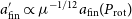
Figure 4 demonstrates the final semimajor axis of the satellite as a function of the assumed planetary rotation period due to the tidal evolution over 10 Gyr. We use the observationally determined minimum mass of the planet ( $m_{p}$
= 2.41 M
$m_{p}$
= 2.41 M $_{\rm J}$
) and a Jupiter-like constant time lag (
$_{\rm J}$
) and a Jupiter-like constant time lag ( $\tau_{p}$
=
$\tau_{p}$
= $\tau_{\rm J}$
) for HD 23079b. The magenta line (with dots) represents this nominal case in Figure 4a and b. The final semimajor axis of the satellite under our nominal conditions is
$\tau_{\rm J}$
) for HD 23079b. The magenta line (with dots) represents this nominal case in Figure 4a and b. The final semimajor axis of the satellite under our nominal conditions is $\sim$
0.0545 R
$\sim$
0.0545 R $_{\rm H}$
for the fastest rotation period (3 h) and
$_{\rm H}$
for the fastest rotation period (3 h) and $\sim$
0.043 R
$\sim$
0.043 R $_{\rm H}$
for the slowest rotation period (12 h). Observations from the RV method restrict the planetary mass measurement to the minimum mass, a limitation that could be overcome in the future. We analyze several other cases that vary the assumed planetary mass by a factor of 1.5 and 2 (see Figure 4a). The satellite’s final semimajor axis
$_{\rm H}$
for the slowest rotation period (12 h). Observations from the RV method restrict the planetary mass measurement to the minimum mass, a limitation that could be overcome in the future. We analyze several other cases that vary the assumed planetary mass by a factor of 1.5 and 2 (see Figure 4a). The satellite’s final semimajor axis $a_{\rm fin}$
decreases for a larger planetary mass (relative to minimum mass
$a_{\rm fin}$
decreases for a larger planetary mass (relative to minimum mass $m_{p}$
) by the mass ratio
$m_{p}$
) by the mass ratio $\mu$
$\mu$ $=m_{p}^\prime/m_{p}$
, which scales by a power law; i.e.,
$=m_{p}^\prime/m_{p}$
, which scales by a power law; i.e., $a_{\rm fin}^\prime \propto \mu^{-1/12}a_{\rm fin}(P_{\rm rot})$
.
$a_{\rm fin}^\prime \propto \mu^{-1/12}a_{\rm fin}(P_{\rm rot})$
.
Relationship between the satellite’s final semimajor axis and the planetary rotation period based on tidal model simulations for different values of $m_{p}$
and
$m_{p}$
and $\tau$
. (a) Results varying the assumed planetary mass (1.0
$\tau$
. (a) Results varying the assumed planetary mass (1.0 $m_{p}$
, 1.5
$m_{p}$
, 1.5 $m_{p}$
, and 2.0
$m_{p}$
, and 2.0 $m_{p}$
) while using a Jupiter-like tidal time lag
$m_{p}$
) while using a Jupiter-like tidal time lag $\tau$
. (b) Results varying the tidal time lag from 0.01
$\tau$
. (b) Results varying the tidal time lag from 0.01 $\tau$
to 100
$\tau$
to 100 $\tau$
. The horizontal line in (b) at 0.015 R
$\tau$
. The horizontal line in (b) at 0.015 R $_{\rm H}$
represents
$_{\rm H}$
represents $3 R_{\mathrm{Roche}}$
. Note the difference in the y-axis ranges between panel (a) and (b). Additionally, the 1
$3 R_{\mathrm{Roche}}$
. Note the difference in the y-axis ranges between panel (a) and (b). Additionally, the 1 $m_{p}$
curve in (a) and the 1
$m_{p}$
curve in (a) and the 1 $\tau$
cure in (b) are identical. In panel (b), only every other calculation has been depicted by a marker for increased clarity of the figure.
$\tau$
cure in (b) are identical. In panel (b), only every other calculation has been depicted by a marker for increased clarity of the figure.
In Figure 4b, we vary the dissipation strength through the constant time lag over four orders of magnitude ( $C_\tau = 10^{-2}-10^{2} \tau$
). Interestingly, a 100-fold increase in
$C_\tau = 10^{-2}-10^{2} \tau$
). Interestingly, a 100-fold increase in $\tau$
(orange squares in Figure 4b) results in a doubling of the final satellite semimajor axis when the planetary rotation period
$\tau$
(orange squares in Figure 4b) results in a doubling of the final satellite semimajor axis when the planetary rotation period $P_{\rm rot}$
is 3 h; i.e.,
$P_{\rm rot}$
is 3 h; i.e., $a_{\rm fin}^\prime \propto C_\tau^{1/6}a_{\rm fin}(P_{\rm rot})$
. The satellite’s semimajor axis evolution (see Equation (3)) depends linearly on the assumed value for
$a_{\rm fin}^\prime \propto C_\tau^{1/6}a_{\rm fin}(P_{\rm rot})$
. The satellite’s semimajor axis evolution (see Equation (3)) depends linearly on the assumed value for $\tau_{ p}$
, but it also depends non-linearly on
$\tau_{ p}$
, but it also depends non-linearly on $\tau_{p}$
through the changes in the planetary rotation rate
$\tau_{p}$
through the changes in the planetary rotation rate $\Omega_{p}$
(see Equation (5)). The combination of those dependencies are the likely underlying cause of the empirically derived scaling relation.
$\Omega_{p}$
(see Equation (5)). The combination of those dependencies are the likely underlying cause of the empirically derived scaling relation.
Irregardless of the assumed parameters for the tidal evolution, the final $a_{\rm sat}$
is far from the stability limit, where the largest final
$a_{\rm sat}$
is far from the stability limit, where the largest final $a_{\rm sat}$
is only
$a_{\rm sat}$
is only $\sim$
1/3 of the prograde stability limit. The tidal force is known to decrease rapidly with distance. Thus, starting the satellite at most separations would not affect the satellite’s potential stability (Quarles et al. Reference Quarles, Li and Rosario-Franco2020b). However, the CTL model considers tidal migration secularly without any interruptions due to MMRs or changes in the internal evolution of the host planet (Touma & Wisdom Reference Touma and Wisdom1998). Realistically, such interactions could include slowing down the migration process temporarily. In fact, this kind of behavior may have occurred for our Moon (Sasaki et al. Reference Sasaki, Barnes and O’Brien2012). Tidal evolution with multiple moons could also induce some volcanic activity as is the case for Io (Peale, Cassen, & Reynolds Reference Peale, Cassen and Reynolds1979.) and potentially affect an exomoon’s habitability (Heller & Barnes Reference Heller and Barnes2013), but such considerations are beyond the scope of this work.
$\sim$
1/3 of the prograde stability limit. The tidal force is known to decrease rapidly with distance. Thus, starting the satellite at most separations would not affect the satellite’s potential stability (Quarles et al. Reference Quarles, Li and Rosario-Franco2020b). However, the CTL model considers tidal migration secularly without any interruptions due to MMRs or changes in the internal evolution of the host planet (Touma & Wisdom Reference Touma and Wisdom1998). Realistically, such interactions could include slowing down the migration process temporarily. In fact, this kind of behavior may have occurred for our Moon (Sasaki et al. Reference Sasaki, Barnes and O’Brien2012). Tidal evolution with multiple moons could also induce some volcanic activity as is the case for Io (Peale, Cassen, & Reynolds Reference Peale, Cassen and Reynolds1979.) and potentially affect an exomoon’s habitability (Heller & Barnes Reference Heller and Barnes2013), but such considerations are beyond the scope of this work.
3.3. Observability of possible exomoons in the HD 23079 system
The detection of exomoons is currently extremely challenging but their detection is technically feasible, where Sartoretti & Schneider (Reference Sartoretti and Schneider1999) showed the transit method as a promising avenue for their eventual discovery. A dedicated search for exomoons within the Kepler data (Kipping et al. Reference Kipping, Bakos, Buchhave, Nesvorný and Schmitt2012, Reference Jones, Sleep and Chambers2013a,Reference Kipping, Forgan, Hartman, Nesvorný, Bakos, Schmitt and Buchhaveb, Reference Kipping, Nesvorný, Buchhave, Hartman, Bakos and Schmitt2014, Reference Kipping, Schmitt, Huang, Torres, Nesvorný, Buchhave, Hartman and Bakos2015b) has yet to confirm an exomoon, while noting that Kepler 1625b-I represents an interesting candidate (Teachey & Kipping Reference Teachey and Kipping2018). To observe an exomoon in the HD 23079 system, a different approach is required since the host planet was discovered through the RV method (Tinney et al. Reference Tinney, Butler, Marcy, Jones, Penny, McCarthy and Carter2002; Wittenmyer et al. Reference Wittenmyer2020) and is not known to transit its host star relative to our line-of-sight. The expected semi-amplitude $K_{\rm o}$
from the stellar motion about the center-of-mass is
$K_{\rm o}$
from the stellar motion about the center-of-mass is $\sim$
54 m s–1, where the addition of an Earth-mass satellite orbiting HD 23079b would introduce a small additional variation (
$\sim$
54 m s–1, where the addition of an Earth-mass satellite orbiting HD 23079b would introduce a small additional variation ( $<$
1 m s–1). Consequently, the most promising technique is Doppler monitoring within direct imaging observations (Vanderburg et al. Reference Vanderburg, Rappaport and Mayo2018), where an RV signal is extracted from the host planet’s reflex motion after accounting for variations in the host planet’s reflected light.
$<$
1 m s–1). Consequently, the most promising technique is Doppler monitoring within direct imaging observations (Vanderburg et al. Reference Vanderburg, Rappaport and Mayo2018), where an RV signal is extracted from the host planet’s reflex motion after accounting for variations in the host planet’s reflected light.
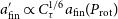
The host planet’s semi-amplitude $K_{p}$
induced by an exomoon (Vanderburg et al. Reference Vanderburg, Rappaport and Mayo2018; Perryman Reference Perryman2018) is given by the following:
$K_{p}$
induced by an exomoon (Vanderburg et al. Reference Vanderburg, Rappaport and Mayo2018; Perryman Reference Perryman2018) is given by the following:
 \begin{equation} K_{p} = \left(\frac{m_{\rm sat}\sin{i_{\rm sat}}}{m_{p} + m_{\rm sat}}\right) \sqrt{\frac{Gm_{\rm sat}}{a_{\rm sat}\left(1-e_{\rm sat}^2\right)}},\end{equation}
where the satellite orbital inclination $i_{\rm sat}$
is relative to the observer’s line-of-sight and should be similar in magnitude to the observed planetary inclination due to tidal evolution of the planet-satellite pair (Porter & Grundy Reference Porter and Grundy2011). Although the system is not known to transit, we assume that
$i_{\rm sat}$
is relative to the observer’s line-of-sight and should be similar in magnitude to the observed planetary inclination due to tidal evolution of the planet-satellite pair (Porter & Grundy Reference Porter and Grundy2011). Although the system is not known to transit, we assume that $i_{\rm sat}=90^\circ$
to estimate the maximum
$i_{\rm sat}=90^\circ$
to estimate the maximum $K_{p}$
. Figure 5 demonstrates the maximum satellite induced
$K_{p}$
. Figure 5 demonstrates the maximum satellite induced $K_{p}$
as a function of the satellite semimajor axis
$K_{p}$
as a function of the satellite semimajor axis $a_{\rm sat}$
in units of R
$a_{\rm sat}$
in units of R $_{\rm H}$
, where the reflex velocity on the planet’s orbit about the barycenter decreases as the satellite semimajor axis increases (
$_{\rm H}$
, where the reflex velocity on the planet’s orbit about the barycenter decreases as the satellite semimajor axis increases ( $K_{p} \propto a_{\rm sat}^{-1/2}$
). The black, red, and blue solid curves mark when an Earth-mass, a standard super-Earth (8 M
$K_{p} \propto a_{\rm sat}^{-1/2}$
). The black, red, and blue solid curves mark when an Earth-mass, a standard super-Earth (8 M $_\oplus$
), or a Neptune (17 M
$_\oplus$
), or a Neptune (17 M $_\oplus$
), respectively, is assumed for the satellite and the RV minimum mass (
$_\oplus$
), respectively, is assumed for the satellite and the RV minimum mass ( $m_{p}=2.41 {\rm M}_{\rm J}$
) is used. The dashed curves are provided to show how much the satellite-induced RV signal decreases, if the assumed planetary mass is doubled (2
$m_{p}=2.41 {\rm M}_{\rm J}$
) is used. The dashed curves are provided to show how much the satellite-induced RV signal decreases, if the assumed planetary mass is doubled (2 $m_{p}$
).
$m_{p}$
).
The RV semi-amplitude $K_{p}$
induced by a satellite with respect to the the planet-satellite semimajor axis
$K_{p}$
induced by a satellite with respect to the the planet-satellite semimajor axis $a_{\rm sat}$
in units of the host planet’s Hill radius R
$a_{\rm sat}$
in units of the host planet’s Hill radius R $_{\rm H}$
. The solid curves represent values assuming the minimum mass (
$_{\rm H}$
. The solid curves represent values assuming the minimum mass ( $m_{p} = 2.41 {\rm M}_{\rm J}$
) is the true planetary mass. The dashed curves illustrate the reduction in
$m_{p} = 2.41 {\rm M}_{\rm J}$
) is the true planetary mass. The dashed curves illustrate the reduction in $K_{p}$
for double the minimum mass (2
$K_{p}$
for double the minimum mass (2 $m_{p}$
). The curves are colour-coded (black, red and blue) to mark the differences in the assumed satellite mass (1, 8 and 17 M
$m_{p}$
). The curves are colour-coded (black, red and blue) to mark the differences in the assumed satellite mass (1, 8 and 17 M $_\oplus$
, respectively).
$_\oplus$
, respectively).
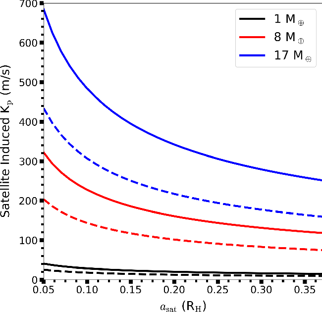
Figure 5 shows that massive ( $\gtrsim$
8 M
$\gtrsim$
8 M $_\oplus$
), prograde-orbiting satellites could produce a Keplerian signal with an RV semi-amplitude greater than
$_\oplus$
), prograde-orbiting satellites could produce a Keplerian signal with an RV semi-amplitude greater than $\sim$
100 m s–1, even with a satellite semimajor axis near the stability limit. Keplerian signals from prograde, Earth-mass satellites are limited to
$\sim$
100 m s–1, even with a satellite semimajor axis near the stability limit. Keplerian signals from prograde, Earth-mass satellites are limited to $\sim$
20–40 m s–1. Retrograde-orbiting satellites stably orbit at larger separations with
$\sim$
20–40 m s–1. Retrograde-orbiting satellites stably orbit at larger separations with $a_{\rm sat} \leq 0.59\:{\rm R}_{\rm H}$
, but the resulting Keplerian signal would be less optimal for the observability.
$a_{\rm sat} \leq 0.59\:{\rm R}_{\rm H}$
, but the resulting Keplerian signal would be less optimal for the observability.
The current best RV precision is $\sim$
1 m s–1, where this precision level is only attainable for bright (
$\sim$
1 m s–1, where this precision level is only attainable for bright ( $V<10$
) stars. The host star in HD 23079 is relatively bright (
$V<10$
) stars. The host star in HD 23079 is relatively bright ( $V=7.12$
; Anderson & Francis Reference Anderson and Francis2012), but the direct imaging method proposed by Vanderburg et al. (Reference Vanderburg, Rappaport and Mayo2018) would allow the analysis of the much fainter reflected light from the planet, which would be much more limited in precision (
$V=7.12$
; Anderson & Francis Reference Anderson and Francis2012), but the direct imaging method proposed by Vanderburg et al. (Reference Vanderburg, Rappaport and Mayo2018) would allow the analysis of the much fainter reflected light from the planet, which would be much more limited in precision ( $\sim$
1 500 m s–1). However, large (30 m class) telescopes (e.g., Giant Magellan Telescope; Jaffe et al. Reference Jaffe, Barnes, Brooks, Lee, Mace, Pak, Park, Park, Evans, Simard and Takami2016) are on the horizon and should be available in the foreseeable future. They would make Doppler surveys of directly imaged planets attainable due to the much larger S/N compared to current technology affecting the RV precision (Quanz et al. Reference Quanz, Crossfield, Meyer, Schmalzl and Held2015). In particular, the detection of Keplerian signals from massive exomoons with an RV semi-amplitude greater than
$\sim$
1 500 m s–1). However, large (30 m class) telescopes (e.g., Giant Magellan Telescope; Jaffe et al. Reference Jaffe, Barnes, Brooks, Lee, Mace, Pak, Park, Park, Evans, Simard and Takami2016) are on the horizon and should be available in the foreseeable future. They would make Doppler surveys of directly imaged planets attainable due to the much larger S/N compared to current technology affecting the RV precision (Quanz et al. Reference Quanz, Crossfield, Meyer, Schmalzl and Held2015). In particular, the detection of Keplerian signals from massive exomoons with an RV semi-amplitude greater than $\sim$
100 m s–1 would be feasible.
$\sim$
100 m s–1 would be feasible.
4. Summary and conclusions
The aim of our study is to further explore the possibility of exomoons in the HD 23079 system. In this system, a solar-type star of spectral class F9.5V hosts a Jupiter-mass planet in a nearly circular orbit situated in the outer segment of the stellar HZ. Previous studies have examined the orbital stability limit of an Earth-mass object in this system as a Trojan planet (Eberle et al. Reference Eberle, Cuntz, Quarles and Musielak2011) or a natural satellite (Cuntz et al. Reference Cuntz, Quarles, Eberle and Shukayr2013). We focus on the latter to more accurately identify the stability limits for prograde and retrograde exomoons within observational constraints, including the recent work by Wittenmyer et al. (Reference Wittenmyer2020).
In the past year, Rosario-Franco et al. (Reference Rosario-Franco, Quarles, Musielak and Cuntz2020) updated the fitting formulas for the stability limit for prograde-orbiting satellites in terms of the planet’s Hill radius, whereas Quarles et al. (Reference Quarles, Eggl, Rosario-Franco and Li2021) improved the fitting formulas for retrograde systems. We follow the prior approaches, in much finer detail, for the HD 23079 system, where the stability limits determined herein specifically exclude regions of quasi-stability and resonances. Additionally, we evaluate multiple satellite mean anomalies, which allows us to overcome some limitations from previous works (e.g., Domingos et al. Reference Domingos, Winter and Yokoyama2006).
Our study shows that the system of HD 23079 is a highly promising candidate for hosting potentially habitable exomoons despite the fact that the outer stability limit is modestly reduced. Noting that HD 23079b’s mass is not exactly known—as due to the RV detection technique only a minimum value could hitherto been identified—our results are still applicable, if a more precise mass value becomes available as the outer orbital stability limit follows a well-defined scaling law, i.e., $(m_{p}^\prime/m_{p})^{1/3}$
; see text for details. The outward migration due to tides does not greatly affect the potential stability of exomoons in a CTL tidal model (Hut Reference Hut1981; Barnes Reference Barnes2017), where we find that a putative satellite’s migration distance the stellar lifetime scales inversely to the 1/12th power in mass ratio
$(m_{p}^\prime/m_{p})^{1/3}$
; see text for details. The outward migration due to tides does not greatly affect the potential stability of exomoons in a CTL tidal model (Hut Reference Hut1981; Barnes Reference Barnes2017), where we find that a putative satellite’s migration distance the stellar lifetime scales inversely to the 1/12th power in mass ratio $\mu$
when comparing different assumptions on planetary mass from the sky plane inclination. Moreover, we find that migration distance scales inversely to the 1/6th power in the assumed tidal time lag parameter
$\mu$
when comparing different assumptions on planetary mass from the sky plane inclination. Moreover, we find that migration distance scales inversely to the 1/6th power in the assumed tidal time lag parameter $\tau$
relative to a Jupiter-like value. Scaling relations, in either the mass or tidal time lag, would assist in the general search for exomoons as well as future observations of the HD 23079 system.
$\tau$
relative to a Jupiter-like value. Scaling relations, in either the mass or tidal time lag, would assist in the general search for exomoons as well as future observations of the HD 23079 system.
We also explore the observability of putative HD 23079 exomoons. Current technologies are incapable of identifying moons in that system; however, future developments hold promise. As the transit method is unavailable for finding exomoons in HD 23079, Doppler monitoring within direct imaging observations might offer positive outcomes. Note that large (30 m class) telescopes (e.g., Giant Magellan Telescope; Jaffe et al. Reference Jaffe, Barnes, Brooks, Lee, Mace, Pak, Park, Park, Evans, Simard and Takami2016) should be available in the foreseeable future. The much larger S/N from telescopes with a large mirror would make Doppler surveys of directly imaged planets attainable, where the Keplerian signals from Earth-mass exomoons with an RV semi-amplitude greater than $\sim$
100 m s–1 would be possible (Vanderburg et al. Reference Vanderburg, Rappaport and Mayo2018).
$\sim$
100 m s–1 would be possible (Vanderburg et al. Reference Vanderburg, Rappaport and Mayo2018).
Acknowledgements
This research was supported in part through research cyberinfrastructure resources and services provided by the Partnership for an Advanced Computing Environment (PACE) at the Georgia Institute of Technology. The authors thank the anonymous reviewer for comments that helped improve the quality and clarity of the manuscript.


