


Impact Statement
This paper addresses generalization limitations with traditional data-driven modeling methods applied to building energy forecasting by introducing a transfer-learning approach that combines physics-based lumped-parameter models in the form of linear state-space models (SSMs) and unsupervised reduced-order modeling methods. Instead of learning black-box models whose generalizability to forecast for unobserved timesteps depends wholly on the representativeness of underlying dynamics in the data, our aim is to leverage the governing structure of low-rank SSMs in a domain adaptation framework. SSMs are well established for building energy forecasting and control purposes and are straightforward to derive from well-known energy transfer ordinary differential equations.
1. Introduction
This paper addresses generalization limitations of traditional data-driven methods when applied to building energy modeling and forecasting. We present a novel transfer-learning (TL) framework that combines physics-based models widely used in the energy community for model predictive control (MPC), with domain adaptation (DA), which is a TL technique typically adopted to leverage pre-trained models for prediction across different but related tasks.
1.1. Building energy modeling and forecasting
The urgency of an ongoing climate crisis in addition to a rising demand for thermal human comfort highlights the need to mitigate energy demand in buildings. Over the last decade, building energy control and operation strategies coupled with innovations in smart grid infrastructures at the urban scale, and controllable energy systems such as heating, ventilation and air-conditioning (HVAC), battery storage, and renewable energy generation at localized building scale, has emerged as a significant approach toward manipulating the energy demand in daily post occupancy operations. On the other hand, advanced energy analysis and optimization methods in preoccupancy stages assist the mitigation of critical design factors influencing both passive and operative energy demand generation. More recently, digital twins that couple energy models with measurement data provide a framework to optimize energy systems of buildings in real time.
Building energy modeling and forecasting plays a vital role in building energy mitigation during both pre and post occupancy stages. A significant volume of past and recent literature (Li and Wen, Reference Li and Wen2014a; Tardioli et al., Reference Tardioli, Kerrigan, Oates, O’Donnell and Finn2015; Bourdeau et al., Reference Bourdeau, Zhai, Nefzaoui, Guo and Chatellier2019) categorize techniques for building energy modeling and forecasting into three main approaches: physics-based, data-driven, and hybrid models. Physics-based models, also known as white-box models (Tardioli et al., Reference Tardioli, Kerrigan, Oates, O’Donnell and Finn2015), are derived directly from mechanistic knowledge of physics principles. Data-driven models, also known as black-box models (ASHRAE, 2009; Tardioli et al., Reference Tardioli, Kerrigan, Oates, O’Donnell and Finn2015), rely on timeseries data and machine-learning (ML) algorithms to accurately learn input–output relationships; these include classic linear regression and more advanced data-driven methods such as random forest (RF) (Wang et al., Reference Wang, Wang, Zeng, Srinivasan and Ahrentzen2018), support vector machine regression (SVR) (Shao et al., Reference Shao, Wang, Bu, Chen and Wang2020) and long short-term memory (LSTM) (Sehovac et al., Reference Sehovac, Nesen and Grolinger2019; Wang et al., Reference Wang, Hong, Xu, Chen, Liu and Xu2019; Somu et al., Reference Somu, M, G and Ramamritham2020). Hybrid models, also referred to as grey-box models (Tardioli et al., Reference Tardioli, Kerrigan, Oates, O’Donnell and Finn2015), are a combination of both physics-based and data-driven models that use simplified physical descriptions of building energy systems via low-rank models and subsequently use data to infer the model parameters via system identification methods; these include resistance–capacitance (RC) thermal networks and state-space models (SSMs) (Candanedo et al., Reference Candanedo, Dehkordi Vahid and Lopez2013; Amara et al., Reference Amara, Agbossou, Cardenas, Dubé and Kelouwani2015; Fateh et al., Reference Fateh, Borelli, Spoladore and Devia2019).
While physics-based models are fully interpretable, they often become infeasible for complex energy systems such as largescale building with several thermal zones because they require large numbers of parameters to be specified, coupled with a computational expense to solve. In such cases, it is typical to either simplify the energy system via hybrid modeling (Goyal and Barooah, Reference Goyal and Barooah2011) or learn an input–output black-box surrogate model via data-driven modeling (Rätz et al., Reference Rätz, Javadi, Baranski, Finkbeiner and Müller2019). The latter has become a widely popular approach for building energy modeling and forecasting due to the recent emergence of ML techniques where given enough data, they are good at finding spatiotemporal patterns and structures even in scenarios where the complexity prohibits analytical descriptions (Willard et al., Reference Willard, Jia, Xu, Steinbach and Kumar2022). In the building energy community, vast literature has demonstrated that ML-based energy modeling methods outperform classic statistical methods in terms of accurately capturing spatiotemporal structures from data for short-term forecasting (Wang et al., Reference Wang, Wang, Zeng, Srinivasan and Ahrentzen2018, Reference Wang, Hong, Xu, Chen, Liu and Xu2019; Sehovac et al., Reference Sehovac, Nesen and Grolinger2019; Shao et al., Reference Shao, Wang, Bu, Chen and Wang2020; Somu et al., Reference Somu, M, G and Ramamritham2020). However, ML-based models are prone to caveats that often impede their application to real-world engineering applications such as real-time monitoring in digital twins (Karpatne et al., Reference Karpatne, Atluri, Faghmous, Steinbach, Banerjee, Ganguly, Shekhar, Samatova and Kumar2017). In this paper, we identify these caveats as (a) model-interpretability, (b) model-generalizability, and (c) data-dependency.
The underlying structure of ML-based models such as for example, deep neural networks, typically take the form of a so-called multi-layer perceptron; a convoluted graph network connecting inputs to outputs. The graph does not hold physical correspondence to mechanistic structures linked with governing phenomena thus render such models difficult to interpret. The network topology and corresponding hyperparameters are typically determined from data using black-box identification techniques. Consequently, the ability for the black-box model to generalize for unseen inputs is heavily influenced by how well the governing behavior of the true system underlying the data is represented in the dataset used for training (not simply on the size of the dataset, as is commonly assumed). If for example, certain occurrences in the dataset are observed more frequently than is characteristic of the true system’s dynamical behavior then, training on such data introduces bias to the model-learning, resulting in poor predictive generalization (Kouw and Loog, Reference Kouw and Loog2018). Since there is no easy way to determine how complete a governing behavior is represented in a dataset or how to control the “representativeness”; black-box models rely on the size of the dataset to secure generalization robustness, in a hit a mis approach. Thus, we can argue that improving the generalizability of typical black-box models for energy forecasting may result in a data-intensive task, which may not be suitable for applied scenarios where for example, obtaining measurement data is challenging or not feasible.
While all caveats need to be addressed, in this paper we focus on addressing generalizability. Specifically, we aim to improve the generalization of building energy models such that we can forecast for unobserved timesteps given building measurement timeseries data. We present an approach that combines physics-derived lumped-parameter models (LPMs) widely adopted in the building energy community for simplified thermal modeling, with DA which is a type of TL technique to leverage pre-trained models for prediction across different but related tasks. In summary, our goal is to forecast for unobserved measurement data by leveraging the generalizability innate in the governing dynamics derived from well-known ordinary differential equations (ODEs) of heat transfer, mechanistically represented as LPMs, even if the latter describes the observed system approximately.
1.2. Lumped-parameter models for building thermal modeling
Thermal modeling of real-world building scenarios may involve high-order intricacies. In scenarios where real-time computation is of essence, such as MPC in digital twins, or iterative computer-based optimization, it becomes infeasible to model and solve such models analytically nor numerically. Instead, LPMs are a popular alternative because they balance out computation time and accuracy while retain mechanistic integrity of the physics to a reasonable degree. Such model simplification methods are also referred to as low-rank models. A popular LPM class of thermal modeling in buildings are RC networks that use an electric circuit analogy to represent the principal energy flow and energy transfer phenomena governing the energy behavior at varying scales; across thermal zones and building components whose behavior is influenced by thermal dynamics (Reference Lin, Middelkoop and BarooahLin et al., 2012; Fayazbakhsh et al., Reference Fayazbakhsh, Bagheri and Bahrami2015; Koeln et al., Reference Koeln, Keating, Alleyne, Price and Rasmussen2018), and across urban scales (Bueno et al., Reference Bueno, Norford, Pigeon and Britter2012). An implementation example of an RC network can be found in the demonstrative example in Section 2. When representing thermal dynamics of a building as an RC network, the capacitors represent thermal capacitance of the air within a zone or the material of a building component, while the resistors represent thermal resistance of the medium between adjacent thermal capacitances (Goyal and Barooah, Reference Goyal and Barooah2012; Amara et al., Reference Amara, Agbossou, Cardenas, Dubé and Kelouwani2015). Once assembled, the network of resistors and capacitors reflect an adjacency network of thermal zones and components via interconnecting energy flow paths. The heat transfer dynamics at each capacitance node can be described by ODEs, whose parameters are either derived from well-known laws of physics or inferred from data through system identification techniques.
In building control applications such as MPC, RC networks are typically formulated in a more mathematically standardized formulation where the coupled system of ODEs in the RC network are written as a linear time-invariant (LTI) SSM, which is a more compact format for representing the mechanistic structure of the transient thermal dynamics that, for example, relates the control signals to the space temperatures and humidity of each zone. Various applications of LTI SSMs to building energy modeling have shown that linear models sufficiently balance out prediction accuracy and model simplicity, as required for MPC (Candanedo et al., Reference Candanedo, Dehkordi Vahid and Lopez2013; Li & Wen, Reference Li and Wen2014b; Picard et al., Reference Picard, Jorissen and Helsen2015). Further literature such as Goyal and Barooah (Reference Goyal and Barooah2012) present a reduced-order modeling (ROM) technique catered for reducing the order of energy SSMs with large number of states, while maintaining a reasonable prediction accuracy. In the case of nonlinearities present in the building energy model due to for example, longwave radiation exchange, absorption of incident solar radiation at the facade, or convective heat transfer, Picard et al. (Reference Picard, Jorissen and Helsen2015) suggest linearization techniques by retaining the nonlinear terms in their state-space formulation.
Despite being linear and approximate, we adopt LTI SSMs in our framework because of their great convenience for control design and estimation, which is justified further by their popularity in the building energy community and by their reasonable robustness in preserving the important dynamics, as illustrated in the above literature. Unlike purely data-driven black-box models, LTI SSMs facilitate access to the mechanistic structure responsible for governing the observed dynamics, even when the physics only describes the dynamics of the system at hand, approximately. It is the innate generalizability thanks to their mechanistic structure, which we aim to leverage using TL.
1.3. Transfer learning
Transfer learning breaks the notion of traditional ML where the training and testing data must come from the same feature space and similar distributions. In fact, in scenarios, where training data are limited, TL strategies can be useful to adapt a trained model from a different but related task. TL methods can be categorized depending on the availability of labeled data in the source and target domains, as follows: (a) inductive TL, where both source and target labeled data are available; (b) transductive TL, where labeled data are only available at the source domain but limited to no labeled data are available at the target domain; and c) unsupervised TL is similar to inductive learning but assumes no labeled data available. A full description of each of these categories, and further subcategories can be found in an extended survey on TL techniques (Pan and Yang, Reference Pan and Yang2010).
In the building energy community, the application of TL is recent. Most applications aim to overcome the dependency on historical data by transferring or adapting data-driven models trained for buildings with available historical measurement data (labeled data), to forecast energy in physically similar buildings whose historical data is limited (some labeled data) or completely unavailable (unlabeled). For example, Fang et al. (Reference Fang, Gong, Li, Chun, Li and Peng2021) address short-term energy prediction for limited historical data by introducing a hybrid deep TL strategy where LSTM-based extractor is used to infer spatiotemporal features across source and target buildings, respectively. Subsequently a domain-invariant feature space is learned to bring closer the two domains using a domain adaptation neural network (DANN) and thus, the model trained on source building data can be leveraged to predict energy in a target building. Similarly, Ribiero et al. (Reference Ribeiro, Grolinger, ElYamany, Higashino and Capretz2018) introduce a novel TL method based on timeseries multi-feature regression with seasonal and trend adjustments. Their approach can be used for buildings with small data by leveraging data from similar buildings with different distributions and seasonal profiles. Their work was validated using a case study involving energy prediction for a school using additional data from other schools. With a similar goal, Gao et al. (Reference Gao, Ruan, Fang and Yin2020) present a TL approach combining a sequence to sequence (seq2seq) model with a convolutional neural network (CNN), resulting in significant accuracy improvements over the use of standard LSTM given only some data in the target building. Their cross-building approach also collects data from similar buildings in a TL framework and is validated by predicting energy for three government buildings across two cities in China. Mocanu et al. (Reference Mocanu, Nguyen, Kling and Gibescu2016) present a TL approach to predict the energy consumption at the building energy level in a smart grid context without the need of labeled historical data from the target building by combining a deep belief network (DBN) for feature extraction, with an extended reinforcement learning approach for knowledge transfer (KT) between buildings. The DBN estimates continuous states, which are then incorporated into the reinforcement learning methods in a continuous lower-dimensional representation of the energy consumption. The outcomes show that their model generalizes for varying time horizons and resolutions using real data thanks to the generalization power of deep belief networks.
In our approach, we adopt a type of transductive TL technique called subspace-based domain adaptation (SDA), which differs from other TL methods by assuming the existence of a domain-invariant feature space between the source and target domains. Using a transductive approach, we leverage the facility of “labeled data” using the physics-based LTI SSM, by adapting the model to forecast for unobserved timesteps (unlabeled data) beyond measurement data. SDA is also referred to as KT in literature. The authors are not aware of previous applications of SDA to building energy modeling. More generally, we believe DA techniques hold significant untapped benefits for building energy modeling applications, including data-efficient calibration of models and cross-building generalization, to name a few.
SDA is a type of TL approach that involves embedding/projecting source and target data into lower-dimensional vector spaces called subspaces. The source and target subspace are defined by the eigenvectors obtained from the ROM methods, respectively. Subsequently SDA seeks for a geometric transformation that brings the subspaces closer together in the form of a mutual subspace (Pan et al., Reference Pan, Tsang, Kwok and Yang2011). Projecting the respective data onto a lower-dimensional subspace helps to reduce the difference between distributions between domains as much as possible while preserving important properties of the original data, such as geometric and statistical properties.
SDA is widely studied in literature with advantageous applications in fields such as computer vision (Baktashmotlagh et al., Reference Baktashmotlagh, Harandi, Lovell and Salzmann2013; Fernando et al., Reference Fernando, Habrard, Sebban, Tuytelaars and Tuytelaars2013), natural language processing (Blitzer et al., Reference Blitzer, Mcdonald and Pereira2006), and so forth. Most research in SDA goes toward improving the lower-dimensional embedding and/or the subspace alignment (SA) strategies with the ultimate scope of minimizing the distance between source and target. For example, Pan et al. (Reference Pan, Tsang, Kwok and Yang2011) present an SDA approach to find a mutual subspace using transfer component analysis (TCA), which combines feature embedding via principal component analysis (PCA) with maximum mean discrepancy (MMD) to find an optimal shared subspace in which the distribution between source and target domain datasets is minimized. In their work, they discuss both unsupervised and semi-supervised feature extraction approaches, to dramatically reduce distance between domain distributions by projecting data onto the learned transfer components. In another approach, Huang et al. (Reference Huang, Yeh and Wang2012) adopt canonical correlation analysis (CCA) to infer a correlation subspace as a mutual representation of action models captured by different cameras for cross-view action/gesture recognition. Elhadji-Ille-Gado et al. (Reference Elhadji-Ille-Gado, Grall-Maes and Kharouf2017) introduce an SDA framework where source and target domains are embedded, respectively, into subspaces described by eigenvector matrices via an approximated singular value decomposition (SVD) method. Subsequently, the source subspace eigenvectors are reoriented to align closer towards the target eigenvectors via SA, resulting in a target-aligned source subspace. In a similar approach, Fernando et al. (Reference Fernando, Habrard, Sebban, Tuytelaars and Tuytelaars2013 and Sebban et al. (Reference Sebban, Fernando, Habrard and Tuytelaars2014) present a closed form method leading to a mapping function (transformation matrix) that aligns source subspace with target subspace vector bases, respectively derived via PCA. By aligning the bases of the subspaces, their approach is global.
1.4. Proposed approach: A physics-based domain adaptation framework
Drawing inspiration from the above approaches, in this paper we present an SDA framework similar to Fernando et al. (Reference Fernando, Habrard, Sebban, Tuytelaars and Tuytelaars2013) and Sebban et al. (Reference Sebban, Fernando, Habrard and Tuytelaars2014). However, instead of leveraging labeled data from a source subspace, we leverage the structure of LPMs widely adopted for thermal modeling of buildings and building components, as discussed in Section 1.2. More specifically, instead of a source subspace derived from labeled data, we derive the subspace directly from the eigenvectors governing the structure of the LTI SSM whose parameters are derived analytically from well-known heat transfer ODEs. On the other hand, we describe the target subspace by the eigenvectors inferred from the measurement data via unsupervised ROM methods such as principal orthogonal decomposition (POD). Once both source and target subspaces are derived, we embed LTI SSM-simulated data (source) and observed measurement data (target) onto their respective lower-dimensional subspaces defined by the respective eigenvectors, and subsequently seek for a geometric transformation that brings the source subspace closer toward the target subspace. In dynamical systems theory, eigenvectors hold direct correspondence with the structure governing the dynamical behavior. Thus, projecting source and target data onto their respective subspaces spanned by their respective eigenvectors, reduces the distance between the respective systems while facilitates a more data-efficient transfer. In Section 5, we illustrate how the SDA approach can be used to forecast unobserved timesteps beyond available measurement data using both near and distant physics-based approximations of the observed system.
In more detail, our physics-based SDA approach via SA can be organized into the following steps (see Figure 1): (1) specify the physics-based model, (2) center the data, (3) infer the source subspace, (4) infer the target subspace, (5) learn the transformation map to align the source subspace with the target subspace, and finally (6) project the source data onto the target-aligned source subspace to forecast the target domain.
Overall subspace-alignment-based domain adaptation (SDA) workflow.

1.5. Outline
In Section 2, we introduce a demonstrative scenario concerning a simple thermal system that will be carried through the paper. In Section 3, we describe the specification of the physics-based SSM (step 1). Subsequently, in Section 4, we describe the proposed subspace-based alignment (steps 2 to 5). Finally, in Section 5, we apply the proposed approach to the demonstrative scenario and discuss the results.
2. Demonstrative Example
We consider a demonstrative building energy system consisting of the thermal conductance through an external wall (outlined in red in Figure 2a) of a single thermal zone. The principal energy dynamics governing the energy transfer through the external wall are represented by the RC network in Figure 2b, where $ {T}_{ext} $
,
$ {T}_{ext} $
, $ {T}_{\mathit{\operatorname{ext}}2} $
,
$ {T}_{\mathit{\operatorname{ext}}2} $
, $ {T}_{\mathit{\operatorname{ext}}1} $
, and
$ {T}_{\mathit{\operatorname{ext}}1} $
, and $ {T}_{int} $
, represent the external ambient temperature, the external surface temperature, the internal surface temperature, and the internal ambient temperature, respectively. In thermal RC networks, the spatial location of the nodes is typically selected with strategic intent for the identification of hidden thermal states of interest that may not be observed or measured directly. For example, in the RC representation of walls, the node locations are typically assigned between the discretized layers composing the construction of the wall to represent the state of interaction between adjacent thermal layers thus, capture the hidden states that play a role in governing the observable dynamic behavior. In our demonstrative example in Figure 2, nodes
$ {T}_{int} $
, represent the external ambient temperature, the external surface temperature, the internal surface temperature, and the internal ambient temperature, respectively. In thermal RC networks, the spatial location of the nodes is typically selected with strategic intent for the identification of hidden thermal states of interest that may not be observed or measured directly. For example, in the RC representation of walls, the node locations are typically assigned between the discretized layers composing the construction of the wall to represent the state of interaction between adjacent thermal layers thus, capture the hidden states that play a role in governing the observable dynamic behavior. In our demonstrative example in Figure 2, nodes $ {T}_{\mathit{\operatorname{ext}}2} $
and
$ {T}_{\mathit{\operatorname{ext}}2} $
and $ {T}_{\mathit{\operatorname{ext}}1} $
were selected with the intention to capture the conductive transfer behavior governed by the thermophysical properties of the wall and represented by the thermal resistor where
$ {T}_{\mathit{\operatorname{ext}}1} $
were selected with the intention to capture the conductive transfer behavior governed by the thermophysical properties of the wall and represented by the thermal resistor where $ {R}_{\operatorname{ext}2\_\operatorname{ext}1}=1/{U}_{\operatorname{ext}2\_\operatorname{ext}1}{R}_{\operatorname{ext}2\_\operatorname{ext}1} $
. The external wall separates two volumes of air where, the thermal resistors
$ {R}_{\operatorname{ext}2\_\operatorname{ext}1}=1/{U}_{\operatorname{ext}2\_\operatorname{ext}1}{R}_{\operatorname{ext}2\_\operatorname{ext}1} $
. The external wall separates two volumes of air where, the thermal resistors $ {R}_{\mathit{\operatorname{ext}}\_\mathit{\operatorname{ext}}2} $
represents the convective heat transfer between external air and external wall surface while and
$ {R}_{\mathit{\operatorname{ext}}\_\mathit{\operatorname{ext}}2} $
represents the convective heat transfer between external air and external wall surface while and $ {R}_{\mathit{\operatorname{ext}}1\_\mathit{\operatorname{int}}} $
represents the convective heat transfer between the inner wall surface and internal room air. Note, that we assume a one-dimensional heat flow through the wall while we ignore the influence of solar radiation acting on the outer surface of the wall. The lumped RC network in Figure 2b is commonly labeled as the 3R2C configuration (three resistors and two capacitors) and is a well-established and validated simplified model for simulating energy behavior of building envelopes and roofs for MPC applications in building management systems (Haves et al., Reference Haves, Norford and DeSimone1998).
$ {R}_{\mathit{\operatorname{ext}}1\_\mathit{\operatorname{int}}} $
represents the convective heat transfer between the inner wall surface and internal room air. Note, that we assume a one-dimensional heat flow through the wall while we ignore the influence of solar radiation acting on the outer surface of the wall. The lumped RC network in Figure 2b is commonly labeled as the 3R2C configuration (three resistors and two capacitors) and is a well-established and validated simplified model for simulating energy behavior of building envelopes and roofs for MPC applications in building management systems (Haves et al., Reference Haves, Norford and DeSimone1998).
(a) Thermal zone for context. (b) Thermal RC network model of one-dimensional energy transfer through an external wall.

We can model the system of nodes algebraically using the general heat balance equation, given by
 $$ \frac{d{T}_j}{dt}=\frac{1}{C_j}\left[\sum \frac{1}{R_k}\left({T}_k-{T}_j\right)+\sum {Q}_j\right], $$
where, $ j $
and
$ j $
and $ k $
represent two adjacent thermal nodes;
$ k $
represent two adjacent thermal nodes; $ {C}_j $
represents the thermal storage capacity at node
$ {C}_j $
represents the thermal storage capacity at node $ j $
;
$ j $
; $ R $
represents the thermal resistance connecting
$ R $
represents the thermal resistance connecting $ j $
and
$ j $
and $ k $
;
$ k $
; $ Q $
represent heat gains from external sources such as lighting and equipment. For the simple wall scenario, we assume a homogenous 1D energy conduction through the wall while ignore heat gains
$ Q $
represent heat gains from external sources such as lighting and equipment. For the simple wall scenario, we assume a homogenous 1D energy conduction through the wall while ignore heat gains $ Q $
from the zone adjacent to the inner surface of the wall. Using equation (1), we can derive the respective energy balance equations for each node [
$ Q $
from the zone adjacent to the inner surface of the wall. Using equation (1), we can derive the respective energy balance equations for each node [ $ {T}_{\mathit{\operatorname{ext}}1},{T}_{\mathit{\operatorname{ext}}2} $
] in the 1D wall scenario as follows:
$ {T}_{\mathit{\operatorname{ext}}1},{T}_{\mathit{\operatorname{ext}}2} $
] in the 1D wall scenario as follows:
 $$ \frac{d{T}_{\mathit{\operatorname{ext}}1}}{dt}=\frac{1}{C_{\mathit{\operatorname{ext}}1}}\left[\frac{1}{R_{\mathit{\operatorname{ext}}{2}_{\mathit{\operatorname{ext}}1}}}\left({T}_{\mathit{\operatorname{ext}}1}-{T}_{\mathit{\operatorname{ext}}2}\right)\right], $$
 $$ \frac{d{T}_{\mathit{\operatorname{ext}}2}}{dt}=\frac{1}{C_{\mathit{\operatorname{ext}}2}}\left[\frac{1}{R_{\mathit{\operatorname{ext}}2\_\mathit{\operatorname{ext}}1}}\left({T}_{\mathit{\operatorname{ext}}1}-{T}_{\mathit{\operatorname{ext}}2}\right)+\frac{1}{R_{\mathit{\operatorname{ext}}\_\mathit{\operatorname{ext}}2}}\left({T}_{\mathit{\operatorname{ext}}2}-{T}_{ext}\right)\right]. $$
The $ R $
and
$ R $
and $ C $
parameters can either be identified using various black-box system identification optimization methods (Madsen, Reference Madsen1995; Candanedo et al., Reference Candanedo, Dehkordi Vahid and Lopez2013; Sarkar et al., Reference Sarkar, Rakhlin and Dahleh2021) from numerically-simulated or empirically-measured data or can be derived directly from first principles. Given our aim to leverage physics-derived knowledge of phenomenon, we derive
$ C $
parameters can either be identified using various black-box system identification optimization methods (Madsen, Reference Madsen1995; Candanedo et al., Reference Candanedo, Dehkordi Vahid and Lopez2013; Sarkar et al., Reference Sarkar, Rakhlin and Dahleh2021) from numerically-simulated or empirically-measured data or can be derived directly from first principles. Given our aim to leverage physics-derived knowledge of phenomenon, we derive $ R $
and
$ R $
and $ C $
directly from first principles of heat storage capacitance, convective resistance, and conductive resistance using well-established mechanisms (equations (4)–(6)).
$ C $
directly from first principles of heat storage capacitance, convective resistance, and conductive resistance using well-established mechanisms (equations (4)–(6)).
 $$ C= Cp\;\rho\;V, $$
 $$ {R}_{conv}=\frac{1}{h\;A,} $$
 $$ {R}_{cond}=\frac{kA}{w/2}. $$
Assigned physical and thermodynamic properties for the 1D wall scenario.

3. Specification of the Physics-Based Model (Step 1)
The first step in our SDA approach is the specification of the physics-based model. In contrast to standard SDA approaches discussed earlier, in our approach, we assume a physics-based LPM as the source domain. More specifically, we assume a physics-derived LTI SSM which offers a standardized representation of dynamical systems and has been shown to capture governing behavior of energy in buildings accurately even when parameters are lumped (Goyal et al., Reference Goyal, Liao and Barooah2011; Goyal and Barooah, Reference Goyal and Barooah2012). Furthermore, lumped SSMs for building thermal network representations can be relatively straightforward to implement.
3.1. LTI SSM
We can further represent the coupled ODEs in equations (2) and (3) in state-space form which is a more compact format to represent the mechanistic structure of the dynamics. SSMs are a standardized representation to describe the dynamics of any system which can be described by a set of ODEs or partial differential equations (PDEs) (Hendricks et al., Reference Hendricks, Jannerup and Sorensen2008). In general, SSMs consist of two matrix equations: the state equation (equation (7)) describes how the inputs influence the states of the system while the output equation (equation (8)) describes how the states of the system and the external factors (inputs) directly influence the observed output of the system. In this paper, we focus on discrete-time LTI SSMs which have the following form:
 $$ x(t)=\left[A\right]\cdot x\left(t-1\right)+\left[B\right]\cdot u\left(t-1\right), $$
 $$ y(t)=\left[C\right]\cdot x\left(t-1\right)+\left[D\right]\cdot u\left(t-1\right). $$
LTI implies that the coefficient parameters do not vary with time. From here on, it is implied that SSM refers to LTI SSM. SSMs are written in terms of three vectors: a state vector $ x $
with
$ x $
with $ n $
elements; an input vector
$ n $
elements; an input vector $ u $
with
$ u $
with $ p $
elements; and an output vector
$ p $
elements; and an output vector $ y $
with
$ y $
with $ q $
elements. Such a state-space formulation is equivalent to the well-known finite difference method. We find that the SSM formulation provides a compact and standardized format to preserve the interpretable structure of governing dynamics, with focus for KT purposes described in Section 3.
$ q $
elements. Such a state-space formulation is equivalent to the well-known finite difference method. We find that the SSM formulation provides a compact and standardized format to preserve the interpretable structure of governing dynamics, with focus for KT purposes described in Section 3.
When representing RC thermal networks as SSMs, we can adopt the temperatures at the capacitance nodes in the RC network as the state variables in the state vector $ x $
, to maintain the same intuitive interpretation (Candanedo et al., Reference Candanedo, Dehkordi Vahid and Lopez2013). In our example wall scenario, the temperature on the internal surface of the wall is our variable of interest and thus, we consider state
$ x $
, to maintain the same intuitive interpretation (Candanedo et al., Reference Candanedo, Dehkordi Vahid and Lopez2013). In our example wall scenario, the temperature on the internal surface of the wall is our variable of interest and thus, we consider state $ {T}_{\mathit{\operatorname{ext}}1} $
as the output variable
$ {T}_{\mathit{\operatorname{ext}}1} $
as the output variable $ y $
while
$ y $
while $ {T}_{ext} $
as the control input
$ {T}_{ext} $
as the control input $ u $
, as follows:
$ u $
, as follows:
 $$ x=\left[\begin{array}{c}{T}_{\mathit{\operatorname{ext}}1}\\ {}{T}_{\mathit{\operatorname{ext}}2}\end{array}\right],\hskip0.5em u=\left[\begin{array}{c}{T}_{ext}\end{array}\right],\hskip0.5em y=\left[\begin{array}{c}\begin{array}{c}{T}_{\mathit{\operatorname{ext}}1}\end{array}\end{array}\right]. $$
These vectors are linked by four coefficient matrices, $ A $
(
$ A $
( $ n\times n $
),
$ n\times n $
), $ B $
(
$ B $
( $ n\times p $
),
$ n\times p $
), $ C $
(
$ C $
( $ q\times n $
), and
$ q\times n $
), and $ D $
(
$ D $
( $ q\times p $
) that capture the dynamic temporal behavior between states
$ q\times p $
) that capture the dynamic temporal behavior between states $ x $
, inputs
$ x $
, inputs $ u $
, and output
$ u $
, and output $ y $
. More specifically,
$ y $
. More specifically, $ A $
is referred to as the dynamics operator which contains the dynamical characteristics to advance the state matrix
$ A $
is referred to as the dynamics operator which contains the dynamical characteristics to advance the state matrix $ x $
from in equation (7) from
$ x $
from in equation (7) from $ x(t) $
to
$ x(t) $
to $ x\left(t+1\right) $
, for time step
$ x\left(t+1\right) $
, for time step $ dt $
, for any arbitrary
$ dt $
, for any arbitrary $ x(t) $
.
$ x(t) $
. $ B $
determines how the influences from control signals, for example, the outdoor air temperature, affect the states, for example, the inner and outer wall surface temperatures. The zero values in
$ B $
determines how the influences from control signals, for example, the outdoor air temperature, affect the states, for example, the inner and outer wall surface temperatures. The zero values in $ B $
indicate that the outdoor temperature
$ B $
indicate that the outdoor temperature $ {\displaystyle \begin{array}{c}\begin{array}{c}{T}_{ext}\end{array}\end{array}} $
influences the internal wall surface temperature
$ {\displaystyle \begin{array}{c}\begin{array}{c}{T}_{ext}\end{array}\end{array}} $
influences the internal wall surface temperature $ {\displaystyle \begin{array}{c}\begin{array}{c}{T}_{\mathit{\operatorname{ext}}1}\end{array}\end{array}} $
by conduction through the wall, not directly. The coefficient values of
$ {\displaystyle \begin{array}{c}\begin{array}{c}{T}_{\mathit{\operatorname{ext}}1}\end{array}\end{array}} $
by conduction through the wall, not directly. The coefficient values of $ A,B,C,D $
are determined directly using the heat balance equations at each node. Thus, the coefficients for the wall example are determined via equations (2) and (3) and as follows:
$ A,B,C,D $
are determined directly using the heat balance equations at each node. Thus, the coefficients for the wall example are determined via equations (2) and (3) and as follows:
 $$ A=\left[\begin{array}{cc}\frac{-{U}_{\mathit{\operatorname{ext}}1,\mathit{\operatorname{ext}}2}}{C_{\mathit{\operatorname{ext}}1}}\;& \frac{U_{\mathit{\operatorname{ext}}1,\mathit{\operatorname{ext}}2}}{C_{\mathit{\operatorname{ext}}1}}\\ {}\begin{array}{c}\frac{U_{\mathit{\operatorname{ext}}1,\mathit{\operatorname{ext}}2}}{C_{\mathit{\operatorname{ext}}2}}\;\end{array}& \begin{array}{c}\frac{-{U}_{\mathit{\operatorname{ext}}1,\mathit{\operatorname{ext}}2}-{U}_{\mathit{\operatorname{ext}}2,\mathit{\operatorname{ext}}}}{C_{\mathit{\operatorname{ext}}2}}\end{array}\end{array}\right],\hskip1em B=\left[\begin{array}{c}\begin{array}{c}0\end{array}\\ {}\frac{U_{\mathit{\operatorname{ext}}2\;\mathit{\operatorname{ext}}}}{C_{\mathit{\operatorname{ext}}2}}\end{array}\right],C=\left[\begin{array}{c}1\\ {}0\end{array}\right],\;D=\left[0\right]. $$
3.2. Structure of the governing state space
A state-space representation allows for a more geometric understanding of dynamical systems. The operator $ A $
can be decomposed into its fundamental components by
$ A $
can be decomposed into its fundamental components by
 $$ AV= V\lambda, $$
where, $ V $
and
$ V $
and $ \lambda $
are the eigenvectors
$ \lambda $
are the eigenvectors $ {v}_1,{v}_2 $
and eigenvalues
$ {v}_1,{v}_2 $
and eigenvalues $ {\lambda}_1,{\lambda}_2 $
of describing the dynamics of
$ {\lambda}_1,{\lambda}_2 $
of describing the dynamics of $ A $
, respectively. The system
$ A $
, respectively. The system $ A $
can then be solved for any timestep
$ A $
can then be solved for any timestep $ dt $
and initial condition
$ dt $
and initial condition $ x\left({t}_0\right) $
by solving the matrix exponential method as follows:
$ x\left({t}_0\right) $
by solving the matrix exponential method as follows:
 $$ {\Phi}_A={e}^{dt A}=V{e}^{dt\lambda}{V}^{-1}, $$
 $$ \dot{x}(t)={e}^{tA}x\left({t}_0\right), $$
where $ {\Phi}_A $
is referred to as the state transition matrix; the matrix that updates the state vector from one timestep to the next. The eigenvalues lie on the diagonal of the
$ {\Phi}_A $
is referred to as the state transition matrix; the matrix that updates the state vector from one timestep to the next. The eigenvalues lie on the diagonal of the $ A $
matrix. Thus, when computing the matrix exponential, we are scaling/transforming the eigenvalues to a given timescale,
$ A $
matrix. Thus, when computing the matrix exponential, we are scaling/transforming the eigenvalues to a given timescale, $ dt $
.
$ dt $
.
We demonstrate the generalizability and interpretability of this physics-derived model using portrait analysis, which is a qualitative analysis method from dynamical system theory to visualize the structure and solutions of dynamical systems geometrically, as trajectories in a vector field. Using portrait analysis, we aim to illustrate how $ V $
and
$ V $
and $ \lambda $
govern the global physical behavior of dynamics, in our case, thermal conduction through the façade wall of a building.
$ \lambda $
govern the global physical behavior of dynamics, in our case, thermal conduction through the façade wall of a building.
In portrait analysis, instead of viewing the state variables $ \left({T}_{\mathit{\operatorname{ext}}1},{T}_{\mathit{\operatorname{ext}}2}\right) $
independently as functions of time (as a timeseries in Figure 3a), we can view their values as coordinates of a point in a vector space bound by
$ \left({T}_{\mathit{\operatorname{ext}}1},{T}_{\mathit{\operatorname{ext}}2}\right) $
independently as functions of time (as a timeseries in Figure 3a), we can view their values as coordinates of a point in a vector space bound by $ {T}_{\mathit{\operatorname{ext}}1},{T}_{\mathit{\operatorname{ext}}2} $
called the state space (Figure 3b). Thus, a point in the state space represents the complete state of the system at any time
$ {T}_{\mathit{\operatorname{ext}}1},{T}_{\mathit{\operatorname{ext}}2} $
called the state space (Figure 3b). Thus, a point in the state space represents the complete state of the system at any time $ t $
. As the system evolves over time, the point will trace out a curve in the state space, referred to as a trajectory. Figure 3b illustrates the traced trajectory in the state space for 300 hourly timesteps for an exemplary scenario where initial internal
$ t $
. As the system evolves over time, the point will trace out a curve in the state space, referred to as a trajectory. Figure 3b illustrates the traced trajectory in the state space for 300 hourly timesteps for an exemplary scenario where initial internal $ \left({T}_{\mathit{\operatorname{ext}}1}\right) $
and external
$ \left({T}_{\mathit{\operatorname{ext}}1}\right) $
and external $ \left({T}_{\mathit{\operatorname{ext}}2}\right) $
wall surface temperature conditions (time
$ \left({T}_{\mathit{\operatorname{ext}}2}\right) $
wall surface temperature conditions (time $ t=0 $
) started at 10.73 and 10.82
$ t=0 $
) started at 10.73 and 10.82 $ {}^{\circ}C $
, respectively. This exemplary initial state scenario could correspond to a situation where an indoor zone experiences heat loss after being recently ventilated (e.g., due to open window for long period of time) causing the internal zone air temperature to drop closer toward the outdoor temperature.
$ {}^{\circ}C $
, respectively. This exemplary initial state scenario could correspond to a situation where an indoor zone experiences heat loss after being recently ventilated (e.g., due to open window for long period of time) causing the internal zone air temperature to drop closer toward the outdoor temperature.
(a) SSM-generated timeseries measurement data plotted as a function of time. (b) SSM-generated timeseries measurement data plotted in the state space.

The behavior of the trajectory observed in Figure 3b can be described as a linear combination of thermal conduction dynamics between $ {T}_{\mathit{\operatorname{ext}}1} $
and
$ {T}_{\mathit{\operatorname{ext}}1} $
and $ {T}_{\mathit{\operatorname{ext}}2} $
, and the influence of the ambient temperature
$ {T}_{\mathit{\operatorname{ext}}2} $
, and the influence of the ambient temperature $ {T}_{ext} $
, as described by the state equation in equation (7). In terms of control systems theory,
$ {T}_{ext} $
, as described by the state equation in equation (7). In terms of control systems theory, $ {T}_{ext} $
can be described as a control forcing signal. Therefore, if we decouple the
$ {T}_{ext} $
can be described as a control forcing signal. Therefore, if we decouple the $ {T}_{ext} $
from
$ {T}_{ext} $
from $ {T}_{\mathit{\operatorname{ext}}1} $
and
$ {T}_{\mathit{\operatorname{ext}}1} $
and $ {T}_{\mathit{\operatorname{ext}}2} $
, we reveal the trajectory traced by the conduction dynamics alone (blue curve in Figure 4a). We do this by fixing the ambient outdoor temperature to a constant value (0
$ {T}_{\mathit{\operatorname{ext}}2} $
, we reveal the trajectory traced by the conduction dynamics alone (blue curve in Figure 4a). We do this by fixing the ambient outdoor temperature to a constant value (0 $ {}^{\circ}C $
), that is, we consider
$ {}^{\circ}C $
), that is, we consider $ x\left(t+1\right)= Ax $
.
$ x\left(t+1\right)= Ax $
.
(a) State-space vector field. (b) Phase portrait of the state space.

The geometry of the decoupled trajectory describes how the full state of the system approaches steady-state conditions, that is, thermal equilibrium. We can interpret the geometry as follows: shortly after the room was ventilated (initial conditions at time $ t=0 $
), the external surface of the wall (
$ t=0 $
), the external surface of the wall ( $ {T}_{\mathit{\operatorname{ext}}2} $
) experiences a sudden drop in temperature due to a decrease in outdoor ambient temperature. Note that how the internal surface temperature (
$ {T}_{\mathit{\operatorname{ext}}2} $
) experiences a sudden drop in temperature due to a decrease in outdoor ambient temperature. Note that how the internal surface temperature ( $ {T}_{\mathit{\operatorname{ext}}1} $
) starts to drop at a much slower rate due to the thermal resistance of the wall. Finally, the internal surface temperature drops toward zero very rapidly once the thermal capacity of the wall is reached. In other words, the path traced by the trajectory can be interpreted as the dynamical behavior of conduction given the specified thermophysical properties of the wall.
$ {T}_{\mathit{\operatorname{ext}}1} $
) starts to drop at a much slower rate due to the thermal resistance of the wall. Finally, the internal surface temperature drops toward zero very rapidly once the thermal capacity of the wall is reached. In other words, the path traced by the trajectory can be interpreted as the dynamical behavior of conduction given the specified thermophysical properties of the wall.
The velocity and path of the traced trajectory are governed by an underlying vector field which describes the global behavior of any trajectory in the state space. The vector field can be described fully by the governing dynamics matrix $ A $
in the SSM from equation (7). More specifically, the velocity and direction of any coordinate
$ A $
in the SSM from equation (7). More specifically, the velocity and direction of any coordinate $ {T}_{\mathit{\operatorname{ext}}1} $
,
$ {T}_{\mathit{\operatorname{ext}}1} $
, $ {T}_{\mathit{\operatorname{ext}}2} $
in the state-space vector field is a function of the eigenvectors
$ {T}_{\mathit{\operatorname{ext}}2} $
in the state-space vector field is a function of the eigenvectors $ {v}_1,{v}_2 $
and eigenvalues
$ {v}_1,{v}_2 $
and eigenvalues $ {\lambda}_1,{\lambda}_2 $
composing
$ {\lambda}_1,{\lambda}_2 $
composing $ A $
. In fact, any point in the state space
$ A $
. In fact, any point in the state space $ T=\left({T}_{\mathit{\operatorname{ext}}1},{T}_{\mathit{\operatorname{ext}}2}\right) $
(representing a thermal scenario) can be described as a linear combination of the eigenvectors. The velocity in a thermal state space represents the rate of change of the temperature states over time and is dictated by the eigenvalues also interpreted as “thermal eigenvalues” (Madsen, Reference Madsen1995; Hyun and Wang, Reference Hyun and Wang2019). Thus, by generating solution trajectories for arbitrary initial state combinations
$ T=\left({T}_{\mathit{\operatorname{ext}}1},{T}_{\mathit{\operatorname{ext}}2}\right) $
(representing a thermal scenario) can be described as a linear combination of the eigenvectors. The velocity in a thermal state space represents the rate of change of the temperature states over time and is dictated by the eigenvalues also interpreted as “thermal eigenvalues” (Madsen, Reference Madsen1995; Hyun and Wang, Reference Hyun and Wang2019). Thus, by generating solution trajectories for arbitrary initial state combinations $ T\left({t}_0\right)=\left[{T}_{\mathit{\operatorname{ext}}1}\left({t}_0\right),{T}_{\mathit{\operatorname{ext}}2}\left({t}_0\right)\right] $
, we reveal the structural geometry of the dynamics governing the thermal behavior of the wall in Figure 4b (also known as a phase portrait). It is this innate initial condition generalizability that we aim to leverage for the KT (and this level of physical interpretability for the wider research goal).
$ T\left({t}_0\right)=\left[{T}_{\mathit{\operatorname{ext}}1}\left({t}_0\right),{T}_{\mathit{\operatorname{ext}}2}\left({t}_0\right)\right] $
, we reveal the structural geometry of the dynamics governing the thermal behavior of the wall in Figure 4b (also known as a phase portrait). It is this innate initial condition generalizability that we aim to leverage for the KT (and this level of physical interpretability for the wider research goal).
Note that phase portraits are more typically used to plot the state space of continuous-time systems; however, the plots in this paper are for discrete-time systems as a result of the post matrix exponential of the dynamics matrix $ A $
in equation (12).
$ A $
in equation (12).
Figure 5a,b illustrate the state trajectories for heat transfer through thicker walls, of 0.6 and 1.5 m, respectively. On qualitative comparison with Figure 3a, we can instantly note a change in the geometry of the vector field and consequently the trajectories, governed by a rotational transformation in the respective orthogonal eigenvector pairs. As the wall gets thicker and the combined U-value decreases, the gradient of heat transfer decreases. When comparing the state-space geometry for different wall systems, for example, varying thicknesses, we can instantly observe a mappable/interpolative similarity. The geometric similarity of these independent but related systems begs the question if mechanistic knowledge can be transferred across a range of thermal systems if represented geometrically as such. Furthermore, Figures 15 to 17 in the Supplementary Material illustrate the geometric differences between dynamics of a system derived from first principles and dynamics derived from data dynamics using spectral decomposition techniques. This view opens up a geometric way to approach/develop geometry-based calibraiton techniques. This is the core motivation behind our work and why we look toward DA as a means to transfer mechanistic knowledge.
(a) Heat transfer through 0.6 m thick wall. (b) Heat transfer through 1.5 m thick wall.

4. Physics-Based Domain Adaptation
4.1. Source and target data pre-processing (step 2)
We start by generating a source dataset $ {X}_s\in {\mathbb{R}}^{n\times z} $
, using the physics-based SSM which is computationally inexpensive to run. On the other hand, we assume availability of a set of measurement data
$ {X}_s\in {\mathbb{R}}^{n\times z} $
, using the physics-based SSM which is computationally inexpensive to run. On the other hand, we assume availability of a set of measurement data $ {X}_t\in {\mathbb{R}}^{n\times z} $
which, for this paper, we generate synthetically (from an EnergyPlus model of the same system) as a representation of empirically observed building measurement data. It is our goal to learn a matrix that geometrically aligns
$ {X}_t\in {\mathbb{R}}^{n\times z} $
which, for this paper, we generate synthetically (from an EnergyPlus model of the same system) as a representation of empirically observed building measurement data. It is our goal to learn a matrix that geometrically aligns $ {X}_s $
with
$ {X}_s $
with $ {X}_t $
. Note that in this approach, we assume pairwise correspondence between source and target data points where both are “generated” under the same input conditions.
$ {X}_t $
. Note that in this approach, we assume pairwise correspondence between source and target data points where both are “generated” under the same input conditions.
Subsequently, $ {X}_s $
and
$ {X}_s $
and $ {X}_t $
are split according to a training/testing ratio (
$ {X}_t $
are split according to a training/testing ratio ( $ l/m\Big) $
. The target training set is used to derive the target subspace eigenvectors
$ l/m\Big) $
. The target training set is used to derive the target subspace eigenvectors $ {V}_t $
via one of the ROM methods discussed, and subsequently also used to learn the transformation matrix
$ {V}_t $
via one of the ROM methods discussed, and subsequently also used to learn the transformation matrix $ M $
in step 4. On the other hand, the target test set is used to validate the forecasted data. The size of
$ M $
in step 4. On the other hand, the target test set is used to validate the forecasted data. The size of $ {V}_t $
used to train the ROM may be set independently from the size of
$ {V}_t $
used to train the ROM may be set independently from the size of $ {V}_t $
used to learn the transformation.
$ {V}_t $
used to learn the transformation.
Prior to subspace embedding, the source and target data are centered along the zero mean as specified by equation (14). Centering the data is an important step and critical for SA as it brings closer the source and target distributions before alignment. The training set and testing set are centered independently to avoid prediction bias due to data leakage from training information to testing.
 $$ \overline{X}=\frac{1}{n}\sum \limits_{j=1}^n{X}_j=0. $$
4.2. Infer source subspace (step 3)
In contrast to standard SDA approaches, we derive the basis of the source subspace as eigenvectors $ {V}_s $
inferred directly from the physics-derived low-rank SSM representation of the energy system in step 1, via eigendecomposition of its system matrix
$ {V}_s $
inferred directly from the physics-derived low-rank SSM representation of the energy system in step 1, via eigendecomposition of its system matrix $ A $
. The decomposition is described in terms of the eigenvalue problem in equation (15) where
$ A $
. The decomposition is described in terms of the eigenvalue problem in equation (15) where $ {\lambda}_s $
is a diagonal matrix containing the eigenvalues. In typical SDA applications, the eigenvectors are derived directly from source data via ROM methods and represent the principal directions in which the variance spans. In our case, the eigenvectors (and eigenvalues) hold direct connotation with the governing structure of the state space as illustrated in Section 2 and thus, aid to improve generalizability of the learned transformation when embedding the measurement data into (lower dimensions) subspaces. It is worthy to note that the
$ {\lambda}_s $
is a diagonal matrix containing the eigenvalues. In typical SDA applications, the eigenvectors are derived directly from source data via ROM methods and represent the principal directions in which the variance spans. In our case, the eigenvectors (and eigenvalues) hold direct connotation with the governing structure of the state space as illustrated in Section 2 and thus, aid to improve generalizability of the learned transformation when embedding the measurement data into (lower dimensions) subspaces. It is worthy to note that the $ A $
derived from the thermal RC network is symmetric implying that the eigenvectors are linearly independent and orthogonal.
$ A $
derived from the thermal RC network is symmetric implying that the eigenvectors are linearly independent and orthogonal.
 $$ A={V}_s{\lambda}_s{V_s}^{\hskip-0.5em -1}. $$
4.3. Infer target subspace (step 4)
In our approach, we derive the vector basis of the target subspace $ {V}_t $
, directly from the available measurement data
$ {V}_t $
, directly from the available measurement data $ {X}_t $
via ROM. In this paper, we adopt POD as the ROM method of choice.
$ {X}_t $
via ROM. In this paper, we adopt POD as the ROM method of choice.
POD is a linear and unsupervised ROM method widely employed in various fields including signal analysis and pattern recognition. POD is equivalent to the well-known PCA in that they both employ SVD to decompose the matrix into orthogonal eigenvectors, aka orthogonal modes. These modes are then used to project the original dataset into an optimal lower-dimensionalFootnote 1 approximation. When applied to fields pertaining to dynamic behavior, the eigenvectors obtained are interpreted as characteristic spatial structure also known as modes, which refer to the characteristic structure of the source system, especially in flow dynamics.
In typical SA applications, further method extensions are implemented to account for deriving the ideal dimensionality of source and target subspaces when applying ROM to the source and target data. The same does not apply to our proposed approach, where both source and target eigenvectors correspond directly to the states of the system thus, already exist in the governing dimensionality.
4.4. Subspace alignment (step 5)
The focus of most SDA methods is to learn an optimal matrix transformation operator/s that aligns the source and target subspaces. We explore two alternative sub-methods for SA: standard SA via minimization of the Bergman divergence perspective (Fernando et al., Reference Fernando, Habrard, Sebban, Tuytelaars and Tuytelaars2013) and Procrustes-based SA (Wang and Mahadevan, Reference Wang and Mahadevan2008). A summary of both algorithms used is given by Algorithms 1 and 2 and are further discussed in more detail here.
The classic SA method is the standard DA alignment approach where a linear transformation that maps source subspace to the target one is determined. This is achieved by aligning the basis vectors using a transformation matrix $ M $
from
$ M $
from $ {X}_s $
to
$ {X}_s $
to $ {X}_t $
(
$ {X}_t $
( $ M\in {\mathbb{R}}^{d\times d} $
) which is learned by minimizing the Bergman matrix divergence in equations (16) and (17), where
$ M\in {\mathbb{R}}^{d\times d} $
) which is learned by minimizing the Bergman matrix divergence in equations (16) and (17), where $ {\left\Vert \left..\right\Vert \right.}_F^2 $
is the Frobenius norm. The Frobenius norm is invariant to orthonormal operations and thus can be rewritten as the objective function in equation (19) as suggested by Fernando et al. (Reference Fernando, Habrard, Sebban, Tuytelaars and Tuytelaars2013) and Sebban et al. (Reference Sebban, Fernando, Habrard and Tuytelaars2014).
$ {\left\Vert \left..\right\Vert \right.}_F^2 $
is the Frobenius norm. The Frobenius norm is invariant to orthonormal operations and thus can be rewritten as the objective function in equation (19) as suggested by Fernando et al. (Reference Fernando, Habrard, Sebban, Tuytelaars and Tuytelaars2013) and Sebban et al. (Reference Sebban, Fernando, Habrard and Tuytelaars2014).
 $$ F(M)={\left\Vert {X}_sM-\left.{X}_t\right\Vert \right.}_F^2, $$
 $$ {M}^{\ast }={argmin}_MF(M), $$
 $$ {M}^{\ast }={X_s}^T{X}_t, $$
 $$ F(M)={\left\Vert {X}_sM-\left.{X}_t\right\Vert \right.}_F^2. $$
In the second alignment approach, we adopt Procrustes analysis, which is a classic statistical method typically used for shape analysis and image registration of 2D/3D data, which seeks isotropic dilation and the rigid translation, reflection, and rotation needed to best match one data structure to another. More specifically, Procrustes alignment removes the translational, rotational, and scaling components so that the optimal alignment between source–target instance pairs is found. Instead of finding a single transformation matrix $ M $
, Procrustes manifold alignment (Wang and Mahadevan, Reference Wang and Mahadevan2008; Perron et al., Reference Perron, Rajaram and Mavris2021) seeks to align source and target subspaces using the rotation matrix
$ M $
, Procrustes manifold alignment (Wang and Mahadevan, Reference Wang and Mahadevan2008; Perron et al., Reference Perron, Rajaram and Mavris2021) seeks to align source and target subspaces using the rotation matrix $ r $
$ r $ $ \in {\mathbb{R}}^{n\times n} $
and scaling factor
$ \in {\mathbb{R}}^{n\times n} $
and scaling factor $ s $
, found via Procrustes analysis on the embedded data. First, we project SSM-generated data onto the source eigenvectors, and the target measurement data onto the target eigenvectors,
$ s $
, found via Procrustes analysis on the embedded data. First, we project SSM-generated data onto the source eigenvectors, and the target measurement data onto the target eigenvectors,
 $$ {\overset{\sim }{X}}_s={X}_s{V_s}^T,\hskip1em {\overset{\sim }{X}}_t={X}_t{V_t}^T. $$
Subsequently, we align the two using ordinary Procrustes via the SVD of the embedded datasets:
 $$ U\Sigma {V}^T= SVD\left({{\overset{\sim }{X}}_t}^T{\overset{\sim }{X}}_s\right), $$
 $$ r=U{V}^T, $$
 $$ s=\frac{trace\left(\Sigma \right)}{trace\left({\overset{\sim }{X}}_s{\left({\overset{\sim }{X}}_s\right)}^T\right)}, $$
where $ U\in {\mathbb{R}}^{n\times n} $
and
$ U\in {\mathbb{R}}^{n\times n} $
and $ V\in {\mathbb{R}}^{n\times n} $
are matrices containing the left and right singular vectors and
$ V\in {\mathbb{R}}^{n\times n} $
are matrices containing the left and right singular vectors and $ \Sigma \in {\mathbb{R}}^{n\times 1} $
is a diagonal matrix containing the singular values on its diagonal. Note that in this implementation, we ignore the translation term during Procrustes since given that both
$ \Sigma \in {\mathbb{R}}^{n\times 1} $
is a diagonal matrix containing the singular values on its diagonal. Note that in this implementation, we ignore the translation term during Procrustes since given that both $ {\overset{\sim }{X}}_s $
and
$ {\overset{\sim }{X}}_s $
and $ {\overset{\sim }{X}}_t $
are centered to zero mean prior to subspace embedding. Finally, we reconstruct the original training data by applying
$ {\overset{\sim }{X}}_t $
are centered to zero mean prior to subspace embedding. Finally, we reconstruct the original training data by applying $ r $
and
$ r $
and $ s $
to the embedded source data (equation (24)) and lifting it into the original target space (equation (25)). With this in place, we can forecast for new inputs beyond the available target data.
$ s $
to the embedded source data (equation (24)) and lifting it into the original target space (equation (25)). With this in place, we can forecast for new inputs beyond the available target data.
 $$ {\overset{\sim }{X}}_a= sr{\overset{\sim }{X}}_{s,} $$
 $$ N{X}_a={V_s{\overset{\sim }{X}}_a}^T. $$
Algorithm 1. SA-based DA via Bergman divergence.
Inputs: SSM-generated data $ {X}_s $
, measurement data (simulated)
$ {X}_s $
, measurement data (simulated) $ {X}_{t.} $
Output: Forecasted target data $ {X}_{\hat{t}}. $
-
1. Infer source eigenvectors $ {V}_s $
from the SSM by decomposing
$ A $
, where
$ A={V}_s{\lambda}_s{V_s}^{-1} $
.
$ {V}_s $
from the SSM by decomposing
$ A $
, where
$ A={V}_s{\lambda}_s{V_s}^{-1} $
. -
2. Infer target eigenvectors
$ {V}_t $
from measurement data via POD. -
3. Obtain optimal
$ M $
by aligning
$ {V}_s $
toward
$ {V}_t $
via minimization of the Bergman divergence, where
$ M={argmin}_M\left({\left\Vert {V}_sM-\left.{V}_t\right\Vert \right.}_F^2\right) $
. -
4. Apply
$ M $
to obtain the basis of the new target-aligned subspace
$ {V}_a $
, where
$ {V}_a={V}_s\mathrm{M} $
. -
5. Project source data
$ {X}_s $
onto new target-aligned subspace
$ {V}_a $
, where
$ {\overset{\sim }{X}}_a={X}_s{V_a}^T $
. -
6. Reconstruct aligned source data in target domain, where
$ {X}_a={\overset{\sim }{X}}_a{V}_t $
. -
7. Forecast
$ {X}_{\hat{t}} $
for new inputs by repeating steps 3, 6, and 7.


Algorithm 2. SA-based DA via Procrustes analysis.
Inputs: SSM-generated data $ {X}_s $
, measurement data (simulated)
$ {X}_s $
, measurement data (simulated) $ {X}_t $
.
$ {X}_t $
.
Output: Forecasted target data $ {X}_{\hat{t}}r $
.
$ {X}_{\hat{t}}r $
.
-
1. Infer source eigenvectors
$ {V}_s $
via decomposition of state transition matrix
$ A $
into
$ {V}_s{\lambda}_s{V_s}^{-1}. $
-
2. Infer target eigenvectors
$ {V}_t $
from data via POD. -
3. Project source data
$ {X}_s $
onto source subspace
$ {V}_s $
, where
$ {\overset{\sim }{X}}_s={X}_s{V_s}^T. $
-
4. Project target data
$ {X}_t $
onto target subspace
$ {V}_t $
, where
$ {\overset{\sim }{X}}_t={X}_t{V_t}^T $
. -
5. Infer rotation matrix
$ r $
, scaling factor
$ s $
, and translation factor
$ t $
via Procrustes analysis, where
$ r,s,t= argmin\left({\left\Vert {X}_s-\left.k{X}_tr\right\Vert \right.}_F\right) $
. -
6. Apply
$ r,s,t $
transformations to
$ {\overset{\sim }{X}}_s $
via
$ {\overset{\sim }{X}}_a= rs{\overset{\sim }{X}}_s+t. $
-
7. Reconstruct aligned target data via
$ {X}_a={V}_t{{\overset{\sim }{X}}_a}^T $
. -
8. Forecast
$ {X}_{\hat{t}} $
for new inputs by repeating steps 3, 6, and 7.


4.5. Error metrics
We quantify the performance of the SA-based DA by comparing its prediction accuracy for out of sample inputs, to that of the target data which we consider to be the “true” observed data. More specifically, we compute the coefficient of variation of root-mean-squared error (RMSE) and the normalized mean bias error (NMBE) as follows:
 $$ CV(RMSE)(X)=\frac{1}{\overline{X}}\sqrt{\frac{1}{n}\sum \limits_{i=0}^{n-1}{\left({X}_i-{\hat{X}}_i\right)}^2,} $$
 $$ NMBE(X)=\frac{\sum \limits_{i=0}^{n-1}\left({\hat{X}}_i-{X}_i\right)}{\sum \limits_{i=0}^{n-1}\left({X}_i\right)}. $$
We adopt the guidelines set by the building energy modeling and forecasting community (ASHRAE, 2014) to determine the validity of the RMSE and NMBE results for energy forecasting. For hourly model calibration, it is recommended that maximum allowed NMBE is capped at 10% while the CV(RMSE) at 30%.
5. Demonstrative Application
As aforementioned, we illustrate two application scenarios with the demonstrative wall example: (a) calibration of physics-simulated data to measurement data, and (b) reuse of physics-based model for a variation of wall types undergoing similar phenomenon. For each scenario, we plot and report pre- and post-alignment results via CV(RMSE) and NMBE measures for timeseries reconstruction and forecasting.
5.1. Transfer across equivalent systems (calibration)
We first simulate 7,000 hr of synthetic measurement temperature data for a 0.2 m wall scenario using a high-fidelity simulation model of the thermal zone in Figure 2 using EnergyPlus, which is a widely simulation software used by the building energy community for thermal modeling and simulation. The goal is to calibrate data simulated using a physics-derived SSM model of the same wall scenario (source), closer toward the simulated measurement data (target).
For this study, we select varying training sets from the simulated high-fidelity data: 2,000, 4,000, 6,000 hr. During the simulation, we record the temperature on the inner surface $ {T}_{\mathit{\operatorname{ext}}1} $
and exterior surface
$ {T}_{\mathit{\operatorname{ext}}1} $
and exterior surface $ {T}_{\mathit{\operatorname{ext}}2} $
of the wall at an hourly timestep. Our goal in this exercise is to forecast beyond the measurement data assigned as training (
$ {T}_{\mathit{\operatorname{ext}}2} $
of the wall at an hourly timestep. Our goal in this exercise is to forecast beyond the measurement data assigned as training ( $ {T}_{\mathit{\operatorname{ext}}1} target $
,
$ {T}_{\mathit{\operatorname{ext}}1} target $
, $ {T}_{\mathit{\operatorname{ext}}2} target $
) by leveraging response data (
$ {T}_{\mathit{\operatorname{ext}}2} target $
) by leveraging response data ( $ {T}_{\mathit{\operatorname{ext}}1} source $
,
$ {T}_{\mathit{\operatorname{ext}}1} source $
, $ {T}_{\mathit{\operatorname{ext}}2} source $
) generated from a governing physics-based description (SSM) of the same 0.2 m thick wall scenario, and which is computationally inexpensive to obtain. Note that for clarity, throughout this study we illustrate only the alignment and forecast for the temperature of the inner surface of the wall
$ {T}_{\mathit{\operatorname{ext}}2} source $
) generated from a governing physics-based description (SSM) of the same 0.2 m thick wall scenario, and which is computationally inexpensive to obtain. Note that for clarity, throughout this study we illustrate only the alignment and forecast for the temperature of the inner surface of the wall $ {T}_{\mathit{\operatorname{ext}}1} $
since it is significantly influenced by the conductive dynamics through the wall and thus, of main interest.
$ {T}_{\mathit{\operatorname{ext}}1} $
since it is significantly influenced by the conductive dynamics through the wall and thus, of main interest.
We first specify the elements of the system matrix $ A $
by substituting the thermophysical values for a wall of 0.2 m thickness in Table 1 into equation (9). Subsequently, we obtain the state transition matrix
$ A $
by substituting the thermophysical values for a wall of 0.2 m thickness in Table 1 into equation (9). Subsequently, we obtain the state transition matrix $ {\Phi}_A $
for an hourly timestep
$ {\Phi}_A $
for an hourly timestep $ dt $
by solving
$ dt $
by solving $ {e}^{dtA} $
(equation (29)). Here, we assume an hourly timestep
$ {e}^{dtA} $
(equation (29)). Here, we assume an hourly timestep $ dt=\mathrm{3,600}s $
. Given
$ dt=\mathrm{3,600}s $
. Given $ {\Phi}_A $
, we can obtain the eigenvectors
$ {\Phi}_A $
, we can obtain the eigenvectors $ {V}_{s1},{V}_{s2} $
(specified in Table 5 in the Supplementary Material), via the decomposition in equation (12).
$ {V}_{s1},{V}_{s2} $
(specified in Table 5 in the Supplementary Material), via the decomposition in equation (12).
 $$ A=\left[\begin{array}{cc}-1.2019\mathrm{e}\hskip0.2em -\hskip0.2em 05& 1.2019e\hskip0.2em -\hskip0.2em 05\\ {}1.2019e\hskip0.2em -\hskip0.2em 05& \hskip0.2em -\hskip0.2em 7.879e\hskip0.2em -\hskip0.2em 05\end{array}\right], $$
 $$ {\Phi}_A={e}^{dtA}=\left[\begin{array}{cc}0.95848& -0.03684\\ {}-0.03684& 0.75379\end{array}\right]. $$
Once we compute the basis eigenvectors of the source subspace, we proceed to extract the basis eigenvectors $ {V}_{t1},{V}_{t1} $
of the target subspace from the available measurement data using data-driven ROM. Here, we use POD to infer the basis of the target subspace. The target eigenvectors derived via POD are specified in Table 5 in the Supplementary Material.
$ {V}_{t1},{V}_{t1} $
of the target subspace from the available measurement data using data-driven ROM. Here, we use POD to infer the basis of the target subspace. The target eigenvectors derived via POD are specified in Table 5 in the Supplementary Material.
Now that we have obtained the vector bases for both source and target subspaces, we first project the data generated by the SSM ( $ {T}_{\mathit{\operatorname{ext}}1} source $
,
$ {T}_{\mathit{\operatorname{ext}}1} source $
, $ {T}_{\mathit{\operatorname{ext}}2} source $
) onto the source subspace (onto
$ {T}_{\mathit{\operatorname{ext}}2} source $
) onto the source subspace (onto $ {V}_{s1},{V}_{s2} $
), then project the measurement data (
$ {V}_{s1},{V}_{s2} $
), then project the measurement data ( $ {T}_{\mathit{\operatorname{ext}}1} target $
,
$ {T}_{\mathit{\operatorname{ext}}1} target $
, $ {T}_{\mathit{\operatorname{ext}}2} target $
) onto the target subspace (onto
$ {T}_{\mathit{\operatorname{ext}}2} target $
) onto the target subspace (onto $ {V}_{t1},{V}_{t2} $
), and subsequently proceed to learn a transformation map by aligning the projected source data closer toward the projected target data using the (a) standard SA via Bergman divergence minimization and (b) Procrustes-based SA, described earlier. To reiterate, with (a), we learn a rotational matrix only, while with (b), we learn a rotational matrix, together with scaling and translation factors. Once obtained, the transformation map is first applied to reconstruct the target measurement data used for training by aligning the source data to the target data, and subsequently used to geometrically transform new data generated by the physics-derived SSM into target-aligned data to forecast for 1,000 hr beyond the target measurement data. The CV(RMSE) forecasting results via the standard SA Bergman divergence and Procrustes SA approaches are tabulated in Tables 2 and 4, respectively, to aid comparison between the two alignment approaches for a variety of transfer scenarios. The standard SA Bergmann approach performs poorly at the get-go as can be noted by the CV(RMSE) results. For this reason, in this section, we discuss and illustrate plots for Procrustes-based alignment only.
$ {V}_{t1},{V}_{t2} $
), and subsequently proceed to learn a transformation map by aligning the projected source data closer toward the projected target data using the (a) standard SA via Bergman divergence minimization and (b) Procrustes-based SA, described earlier. To reiterate, with (a), we learn a rotational matrix only, while with (b), we learn a rotational matrix, together with scaling and translation factors. Once obtained, the transformation map is first applied to reconstruct the target measurement data used for training by aligning the source data to the target data, and subsequently used to geometrically transform new data generated by the physics-derived SSM into target-aligned data to forecast for 1,000 hr beyond the target measurement data. The CV(RMSE) forecasting results via the standard SA Bergman divergence and Procrustes SA approaches are tabulated in Tables 2 and 4, respectively, to aid comparison between the two alignment approaches for a variety of transfer scenarios. The standard SA Bergmann approach performs poorly at the get-go as can be noted by the CV(RMSE) results. For this reason, in this section, we discuss and illustrate plots for Procrustes-based alignment only.
CV(RMS) accuracy for forecasting 1,000 hr using standard SA via Bergmann divergence.

Figure 6 illustrates the reconstruction of the internal wall surface temperature $ {T}_{\mathit{\operatorname{ext}}1} $
via Procrustes-based alignment of the physics-derived
$ {T}_{\mathit{\operatorname{ext}}1} $
via Procrustes-based alignment of the physics-derived $ {T}_{\mathit{\operatorname{ext}}1} $
data (red line). Subsequently, the learned transformation was applied to forecast a further 1,000 hr (dotted red line). We note an overall post-alignment improvement in the forecasting CV(RMSE) and NMBE values. We observed that while the physics-derived SSM already approximates the measured system quite well with a CV(RMSE) and NMBE within a desirable bound (≤30 and ≤10%, respectively), our SDA approach improved further these forecasting accuracy values by 1.56 and −3.57%. In the following figures, we also plot the reconstruction and forecasting error (bottom) as a function of localized difference between the aligned and target datapoints (error_postaligned). We compare this with the localized difference between the output from the physics-derived SSM and the target datapoints (error_prealigned).
$ {T}_{\mathit{\operatorname{ext}}1} $
data (red line). Subsequently, the learned transformation was applied to forecast a further 1,000 hr (dotted red line). We note an overall post-alignment improvement in the forecasting CV(RMSE) and NMBE values. We observed that while the physics-derived SSM already approximates the measured system quite well with a CV(RMSE) and NMBE within a desirable bound (≤30 and ≤10%, respectively), our SDA approach improved further these forecasting accuracy values by 1.56 and −3.57%. In the following figures, we also plot the reconstruction and forecasting error (bottom) as a function of localized difference between the aligned and target datapoints (error_postaligned). We compare this with the localized difference between the output from the physics-derived SSM and the target datapoints (error_prealigned).
Calibration scenario: 0.2 m wall SSM (source) to 0.2 m wall data (target). The target subspace was derived via POD (orthogonal eigenvectors).

We repeated the calibration study for a thicker wall (0.8 m) using Procrustes-based SA on 2,000 hr training data. From Table 3, we note that the forecasting accuracy of the aligned (transformed) source data in the 0.8 m wall calibration scenario is 4.49% worse than the original physics-derived SSM (6.34%). We observed improvement for this case when increasing the training data size.
CV(RMS) accuracy for forecasting 1,000 hr using Procrustes-based SA for varying training size (2,000 hr, 4,000 hr, 6,000 hr).
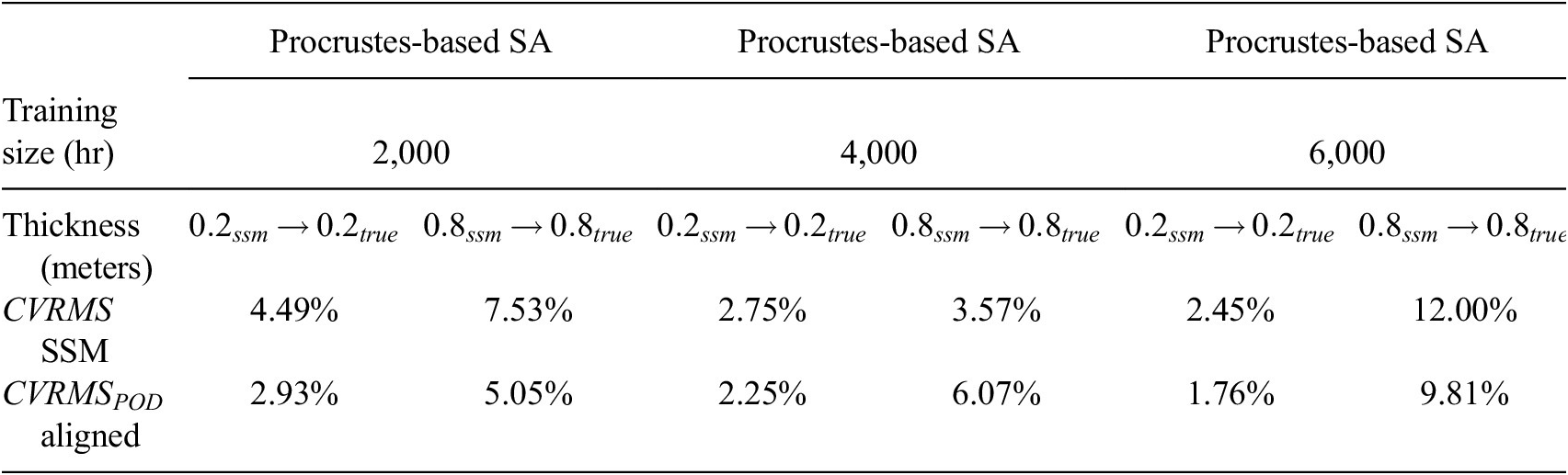
5.2. Transfer across different but related systems (reuse)
We hypothesize that building energy systems governed by similar phenomena have geometrically similar state-space structures implying that their governing subspaces live in a mutual latent space. This suggests that mechanistic descriptions of energy transfer through one wall could be used to describe and forecast the energy transfer through that of a wall with different geometric and material properties, undergoing similar energy transfer phenomena. In this context, we demonstrate how the SDA approach can be used to leverage the low-rank physics-derived SSM of one wall to predict and forecast the internal wall surface temperatures of observed walls with varying thickness and material properties, by learning a SA transformation between physics and given wall surface temperature measurement data.
Figure 7 illustrates the adaptation of a physics-derived SSM for a 0.6 m wall to forecast beyond data observed from a 0.2 m wall via the POD-derived target subspace. The respective source and target eigenvectors can be found in Table 6 in the Supplementary Material.We can immediately observe how the transformation learned between the physics-derived data and the target data has successfully been captured by its ability to reconstruct the training set (red line) when applied to the source data and subsequently to forecast a further 1,000 hr (dotted red line). We utilize the CV(RMSE) and NMBE values to compare the prediction improvement while ensure we are still in desirable bounds typically adopted for building energy model calibration (≤30 and ≤10%, respectively). The improvement can also be noted by observing the difference in pre- and post-alignment error timeseries in the bottom plots.
Cross-domain generalization scenario: 0.6 m wall SSM (source) to 0.2 m wall data (target). The target subspace was derived via POD (orthogonal eigenvectors).

On the other hand, Figure 8 illustrates the adaptation of a physics-derived SSM for a 0.2 m wall to forecast beyond data observed from a 0.6 m wall. While we note forecasting improvement indicating a closer match to the target measurement data, we observe that the transformation via Procrustes alignment does not dampen the noisier source signal. In Section 5.3, we take a closer look to interpret why this occurs.
Cross-domain generalization scenario: 0.2 m wall SSM (source) to 0.6 m wall data (target). The target subspace was derived via POD (orthogonal eigenvectors).

Lastly, Figure 9 illustrates the adaptation of the SSM for a red brick wall of 0.8 m thickness, 0.72 $ W/ mK $
conductivity, 1,920
$ W/ mK $
conductivity, 1,920 $ kg/{m}^3 $
material density, and 780
$ kg/{m}^3 $
material density, and 780 $ J/ kgK $
specific heat capacity, to forecast beyond temperature data measured from a concrete wall of 0.8 m thickness, 1.3
$ J/ kgK $
specific heat capacity, to forecast beyond temperature data measured from a concrete wall of 0.8 m thickness, 1.3 $ W/ mK $
conductivity, 2,240
$ W/ mK $
conductivity, 2,240 $ kg/{m}^3 $
material density, and 840
$ kg/{m}^3 $
material density, and 840 $ J/ kgK $
specific heat capacity. The respective source and target eigenvectors can be found in Table 7 in the Supplementary Material. We can immediately observe that the transformation learned between the SSM and target data is able to forecast the internal surface temperature of the concrete wall for unseen external temperature inputs. This can be noted by the improvements on CV(RMSE) and NMBE values.
$ J/ kgK $
specific heat capacity. The respective source and target eigenvectors can be found in Table 7 in the Supplementary Material. We can immediately observe that the transformation learned between the SSM and target data is able to forecast the internal surface temperature of the concrete wall for unseen external temperature inputs. This can be noted by the improvements on CV(RMSE) and NMBE values.
Cross-domain generalization scenario: 0.8 m red brick wall SSM (source) to 0.3 m concrete wall data (target). The target subspace was derived via POD (non-orthogonal eigenvectors).

5.3. Discussion
The standard SA method via Bergmann divergence minimization does not depend on data because it acts only on the subspaces while Procrustes-based SA acts directly on the local geometry of the projected source and target data. The former only accounts for rotational transformational between source and target subspaces while the latter yields a rotation matrix, skewing, translation, and reflection factors. In Section 5.1 we observed that rotation only is not sufficient to completely describe geometric mappings between subspace-embedded source and target data, particularly in cases where the source and target eigenvectors are in a mirrored orientation from each other. Thus, while we acknowledge that Procrustes-based SA is data-dependent, it is suitable for capturing geometric transformations between physics-derived and measurement timeseries signals, even when transferring across different but related wall-types (Table 4).
CV(RMS) accuracy for forecasting 1,000 hr using cross-domain Procrustes-based SA for varying wall thicknesses only.

We observed that when lifting the target-aligned data from the embedded space to the target space, the source–target alignment can be compromised in cases when the basis of the target-aligned subspace does not align well with the basis of the target subspace. For example, in the cross-domain alignment example ( $ {0.2}_{ssm}\to {0.9}_{true} $
) illustrated in Figure 10, top, we instantly note that Procrustes successfully aligns the source with target signal in the embedded space (left) but the alignment is subsequently compromised when lifting into the target subspace (right). This was evident when comparing the source–target alignment data in the embedded space. Figure 10, bottom, illustrates another instance when this occurs, this time a same-domain alignment scenario.
$ {0.2}_{ssm}\to {0.9}_{true} $
) illustrated in Figure 10, top, we instantly note that Procrustes successfully aligns the source with target signal in the embedded space (left) but the alignment is subsequently compromised when lifting into the target subspace (right). This was evident when comparing the source–target alignment data in the embedded space. Figure 10, bottom, illustrates another instance when this occurs, this time a same-domain alignment scenario.
Top: cross-domain alignment: 0.2 m wall SSM (source) to 0.9 m wall data (target). Middle: same-domain alignment: 0.8 m wall SSM (source) to 0.8 m wall data (target). Left plots illustrate alignment in the embedded space. Right plots illustrate the alignment after lifting from embedded space.

We also experimented with dynamic mode decomposition (DMD) as an alternative ROM method to infer the target subspace. DMD is known to be superior at capturing the governing temporal structure underlying data. DMD was not suitable for all domain transfer cases mainly since the eigenvectors inferred via DMD are non-orthogonal. It is noteworthy that in the successful cases, we observed significant alignment improvement resulting in longer-term forecasts when compared to POD-derived target subspace. This can be observed by comparing Figure 11 in the Supplementary Material with Figure 12 in the Supplementary Material.
While the demonstrative example in this paper assumes a simple building component, the physics-based SDA framework is scalable to model more intricate building systems and or thermal zones. There exists dedicated work to automate the generation of RC networks from 3D models of thermal zones (Reference Kim, Bae, Braun, Travis Horton, Travis and HortonKim et al., 2018). Furthermore, the energy balance equations assumed to inform the SSM are well known by the energy community and straightforward to implement.
While the examples illustrated above do not assume noisy conditions in the measurement data, in Figures 13 and 14 in the Supplementary Material, we illustrate a scenario where random noise was added to the measurement data. In noisy measurement conditions, the modeling goal is not to forecast a noisy signal but rather, to forecast a denoised signal. Thus, bypassing a noisy measurement signal wholly depends on the capability of the ROM method to decouple the noise from the true signal. In the example illustrated by Figures 13 and 14 in the Supplementary Material, we introduce noise sampled from a random distribution with a mean of 0.5 and a standard deviation of 0.9, to the measurement data from the scenario discussed in Section 5.2. We can observe how the SDA approach is able to learn a transformation between the source and a noise-filtered target signal that generalizes successfully beyond measured timesteps. This is largely due to the SVD decomposition of the noisy signal when applying POD to the target data where the SVD acts as a noise filter (Shin et al., Reference Shin, Hammond and White1999; Epps and Krivitzky, Reference Epps and Krivitzky2019). Figures 13 and 14 in the Supplementary Material demonstrate the SA results in the subspace-embedded and the lifted space, respectively. If POD does not suffice for denoising the timeseries data, there exist extensions of POD such as SPOD (Sieber et al., Reference Sieber, Paschereit and Oberleithner2016) that focus on spectral decomposition to deal with such decoupling/filtering more successfully. The main difference between POD and SPOD is that the modes vary in both space and time and are orthogonal under space–time inner product, rather than only spatially.
For stochastic LTI SSMs, the presented SDA approach could be extended by introducing a stochastic noise term to a continuous-time LTI SSM which can subsequently be translated in to discrete-time via integration (Madsen, Reference Madsen1995). Such an implementation would not alter the state transition matrix ( $ A $
matrix) from which we derive the source subspace eigenvectors.
$ A $
matrix) from which we derive the source subspace eigenvectors.
The “adaptability” of a physics-based model to forecast for a target measured system using our presented SDA approach is limited by two factors: (a) The state dimensions in the physics-based model need to be equivalent to the dimensions of the measurement data implying that the resolution of the SSM is limited by the number of available corresponding measurements. In future work, we intend to facilitate prediction of unobserved target measurements by leveraging their corresponding physics-derived state in the SSM. (b) We assume source and target data have pairwise correspondence, implying that the SSM control inputs are the same (measured) control signals known to be influencing the target measurement data, for example, the external ambient temperature from the case study in Section 5. Pairwise correspondence can easily be ensured for MPC applications because most typical building energy scenarios can be described by well-established governing laws, even if approximate.
6. Conclusion
In this paper, we introduced a novel TL approach to address better model-generalization for timeseries forecasting of building energy, by exploiting well-established ODEs governing thermal transfer in a data-driven framework. Our approach combines physics-derived LTI SSMs with SA where a geometric transformation is sought to align the subspace derived from governing physics closer toward the subspace decomposed from the measurement data. Subsequently, the transformation is used to forecast beyond the observed measurement data by transforming physics simulated data for unseen timesteps into approximated measurement data.
While our physics-based SDA framework addresses generalization for unseen timesteps (timeseries forecasting), it can easily be adopted for cross-system generalization where, for example, we can exploit LTI SSMs identified from data (instead of first principles) of a fully observed system to forecast for unseen timesteps given measurement data from a different but related system. Such an approach could benefit data-efficient control strategies across thermal zones or building components within the same building, by transforming LTI SSM models calibrated on specific thermal zones/components to forecast for other different but related thermal zones/components.
In subsequent work, we intend to test the physics-based SDA framework on real observed scenarios and applications pertaining to energy systems and components in buildings. This work stems from a broader research goal where we aim to overcome persisting caveats with traditional data-driven energy modeling and forecasting, namely, generalizability, data-dependency, and interpretability.
Acknowledgments
We are grateful for the technical assistance of Dr. Andrew Duncan.
Author contribution
Conceptualization: Z.X.C., R.C.; Data visualization: Z.X.C.; Formal analysis: Z.X.C., L.M.; Methodology: Z.X.C.; Software: Z.X.C.; Validation: all authors; Writing original draft: Z.X.C. All authors approved the final submitted draft.
Competing interest
The authors declare no competing interests exist.
Data availability statement
The data used throughout this paper were synthetically generated. The authors have ensured to provide sufficient information to replicate the analytical and numerical models used to generate the synthetic data.
Funding statement
This work was supported by The Alan Turing Institute’s Data-Centric Engineering Program under the Lloyd’s Register Foundation Grant G0095, and Wave 1 of The UKRI Strategic Priorities Fund under the EPSRC Grant EP/T001569/1 and EPSRC Grant EP/W006022/1, particularly the digital twins in engineering theme within those grants and The Alan Turing Institute.
Supplementary material
The supplementary material for this article can be found at http://doi.org/10.1017/dce.2023.8.


 Open access
Comments
No Comments have been published for this article.