


Impact Statement
In this article, we provide a hierarchical Bayesian methodology for calibrating mathematical models of complex materials. Importantly, this approach naturally includes experimental data from a set of (potentially different) tests. Using the hierarchical approach, we are able to quantify the population statistics for uncertainties arising from variations of the test, measurement uncertainty, and model misspecification. Our approach is tested on two different test cases, including a real world application for 3D-printed steel, proving both its efficiency and versatility.
1. Introduction
In engineering and across the physical sciences, both in academia and industry, the parameterization of constitutive models for materials from a set of experiments is a very common research question. Parameterization of constitutive models is often used to classify or compare the response of different materials, or as the starting point for establishing mathematical models of the system, in which that material is used such as finite element analysis. The standard approach is to carry out a series of experiments. For each, the parameters which minimize the squared difference between the experiment’s output and the model response are found. This procedure is often called the least squared method (LSM). The population statistics of the derived model parameters over all experimental tests are then computed, and often limited to a simple mean and standard derivation of the samples.
Although very common, the LSM approach requires a sufficient number of experimental tests to establish “good” estimates. This makes it hard to establish good estimates for the distribution of parameters, particularly, if experimental data are limited. Although various contributions have enhanced the LSM method (Charnes et al., Reference Charnes, Frome and Yu1976), statistical information about the measurement uncertainty in the experiment and the model misspecification (i.e., “all models are wrong”) are generally not captured. The simple averaging approach to establishing population statistics, and even more advanced assumptions like taking into account covariances between parameters, also lose much information about the population distribution of the parameters and their often complex interdependencies.
Bayesian model calibration is a popular framework for estimating the values of input parameters into computational simulations in the presence of multiple uncertainties (Kennedy and O’Hagan, Reference Kennedy and O’Hagan2001; Bayarri et al., Reference Bayarri, Berger, Paulo, Sacks, Cafeo, Lin and Tu2007), and provides a formalized way to include prior knowledge of parameters to support cases where there are limited measurement data. They have been applied broadly across many area of science in engineering, healthcare, and ecology (Solonen et al., Reference Solonen, Ollinaho, Laine, Heikki, Johanna and Heikki2012; Thomas et al., Reference Thomas, Redd, Khader, Leecaster, Greene and Samore2015; Valderrama-Bahamóndez and Fröhlich, Reference Valderrama-Bahamóndez and Fröhlich2019). Although less common in engineering, Bayesian approaches have also been used to calibrate material models from experimental data. The first such use, to the best of the authors’ knowledge, was by Isenberg (Isenberg, Reference Isenberg1979),who used it to identify elastic material parameters for a simple model and experimental test. It is only relatively recently that Bayesian-based approaches have been used to parameterize models: elastic constants of composite and laminate plates (Gogu et al., Reference Gogu, Yin, Raphael, Peter, Le Riche, Rodolphe and Vautrin2013), time-dependent material models in viscoelasticity (Rappel et al., Reference Rappel, Beex and Bordas2018), and large strain elastoplastic models for 3D-printed steel (Dodwell et al., Reference Dodwell, Fleming, Buchanan, Kyvelou, Detommaso, Gosling, Scheichl, Gardner, Girolami and Oates2021), to give just a few examples. Beyond the straight probabilistic calibration of material parameters based on a single experiment, Bayesian approaches have been used to access the relatively predictive quality over a family of possible models, so-called Bayesian Model Selection (Chipman et al., Reference Chipman, George, Robert, Clyde, Dean and Stine2001; Johnson and Rossell, Reference Johnson and Rossell2012). Such approaches have had particular impact in a number of computational material science applications, since there are often many choices of possible material model. A Bayesian model selection approach formalizes the material model selection, balancing both prior knowledge and evidence from experimental data. Notable examples include hyperelastic constitutive models for tissue (Madireddy et al., Reference Madireddy, Sista and Vemaganti2015), phenomenological models for tumour growth (Oden et al., Reference Oden, Prudencio and Hawkins-Daarud2013), models of damage progression in composites due to fatigue (Chiachío et al., Reference Chiachío, Chiachio, Saxena, Sankararaman, Rus and Goebel2015), and also for fatigue descriptions of metals (Babuška et al., Reference Babuška, Sawlan, Scavino, Szabó and Tempone2016).
The Bayesian approaches in the literature have focused on the calibration of a material model from a single experiment. In many engineering applications, it is the distribution of possible model parameters derived from a set of experiments, rather than individual experiments, that is of interest. The set of experiments may be generated from different samples of material and tested under different conditions, or multiple tests are repeated to explore the variability in the material and/or the measurement uncertainty in the test itself. If we consider a setting where we have performed  $ J $ experiments of the same material and
  $ {\psi}_j $ represents the model parameters which describe the jth experiment. It is expected that the parameters
  $ {\psi}_j $ and parameters for another experiment
  $ {\psi}_i $ will be positively correlated, since they offer model parameterizations for the same material, albeit in different instances of the same physical experiment. A natural way to build this dependency into a Bayesian setting is to define prior distributions for our material parameters, and see
  $ {\psi}_j $ is seen as themselves samples from a common population distribution over the set of all possibly observable experiments. This population distribution itself can be parameters
  $ \phi $ (referred to as hyper-parameters)—which might are typical population statistics (e.g., mean, variance, or higher moments). In a Bayesian setting, the hyper-parameters themselves are also equipped with a probabilistic specification, and with that they assign themselves prior distributions, hyper-priors. This gives a natural hierarchical representation of multiexperimental parameterization problem. This framework defines a Hierarchical Bayesian Model (HBM) (Gelman et al., Reference Gelman, Carlin, Stern, Dunson, Vehtari and Rubin2013; Figure 1). HBMs have been widely used in statistical applications (Kwon et al., Reference Kwon, Brown and Lall2008; Loredo, Reference Loredo2013; Wolfgang, Reference Wolfgang2016; Bozorgzadeh et al., Reference Bozorgzadeh, Harrison and Escobar2019). Probably, most notably, they have been used in statistics models for drug trials to determine population statistics in response to a new drug when the data received are unique to an individual patient (Babapulle et al., Reference Babapulle, Joseph, Bélisle, Brophy and Eisenberg2004; Huang et al., Reference Huang, Liu and Wu2006).
Model parameters  $ {\psi}_i $ can be calibrated to a specific experimental dataset
  $ {\mathbf{d}}_i $. If repeated over
  $ J $ experiments
  $ \left\{1,\dots, J\right\} $, natural variations in each
  $ {\psi}_i $ would be observed. In this contribution, a hierarchical Bayesian framework is developed which learns the population distribution of the
  $ {\psi}_i $‘s. If this population distribution is parameterized by some hyper-parameters (e.g., in this figure, we assume
 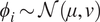 $ {\phi}_i\sim \mathcal{N}\left(\mu, v\right) $, which are themselves equipped with prior distribution, reflecting uncertainty in their values and representation.
As far as the authors are aware, this article sets out the first hierarchical Bayesian framework for the parameterization of material models from a set of experimental data. It starts by recapping the calibration of a material model from a single experimental test (Section 2.1), and then extends the approach to a full set of data (Section 2.2). An efficient computational strategy for ensuring the resulting Markov Chain Monte Carlo (MCMC) computations for the HBM remains feasible and is presented. This uses a simple trick to marginalize all realization of the model parameters for a particular experiment in an offline stage. Online, during MCMC sampling of the hyperparameters, an approximate likelihood can be efficiently estimated. The uncertainty in this approximation is captured using Bayesian Quadrature (O’Hagan, Reference O’Hagan1991; Osborne et al., Reference Osborne, Garnett, Ghahramani, Duvenaud, Roberts and Rasmussen2012) to approximate the marginalization integral. The set of approaches is demonstrated for two examples. The first is a simple analytical model for the calibration of a linear spring, and the second an application of the methodology to a more complex nonlinear hyper-elastic model solved with the help of Finite Element Method, in which real experimental data are used (Gardner et al., Reference Gardner, Kyvelou, Herbert and Buchanan2020).
The results demonstrate that a hierarchical Bayesian framework is a natural setting for the calibration of material constitutive in the model from a set of experiment tests. The approach addresses the limitations of standard, nonprobabilistic approaches (e.g., least square) and enables the capture of measurement, model uncertainties, and complex interdependencies between model parameters, including prior knowledge in cases where data are limited. It provides a framework, in which the population statistics of the material parameters can be estimated, rather than snapshots of individual experiments under the assumption, they are independent and correlation between parameters is not significant.
2. A HBM for Estimating Material Parameters from a set of Experiments
We start this section by first recapping the parameterization of a material model from a single experimental test. This single experiment approach is then extended into a hierarchical Bayesian framework (Gelman et al., Reference Gelman, Carlin, Stern, Dunson, Vehtari and Rubin2013), in which we infer the population statistics of the material parameters from a set of experimental tests. It then considers computationally efficient strategies for implementing the hierarchical approach.
2.1. Bayesian calibration of a material model given a single experiment
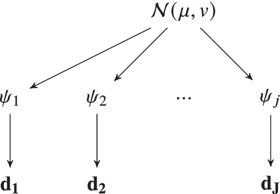
We first set up a Bayesian formulation, from which we can estimate the distribution of material parameters given that we observe the outputs of only a single experiment. Let  $ \boldsymbol{\psi} ={\left({\psi}_1,\dots, {\psi}_m\right)}^T\in \boldsymbol{\unicode{x03C8}} \subset {\mathrm{\mathbb{R}}}^m $ denote a vector of random parameters which define the parameter space
  $ \boldsymbol{\Psi} $ of a particular material model. It is assumed that the material parameters have a prior distribution defined by the density
  $ {\pi}_0\left(\boldsymbol{\psi} \right):\boldsymbol{\unicode{x03C8}} \to {\mathrm{\mathbb{R}}}^{+} $.
Let the recorded outputs of an experimental test be defined by the vector  $ \mathbf{d}={\left({d}_1,\dots, {d}_s\right)}^T\in {\mathrm{\mathbb{R}}}^s $. These, for example, could be the load measurements to achieve a given displacement by the test machine, or the strain measurement from strain sensors or digital image correlation software. Let
  $ \mathbf{f}\left(\boldsymbol{\psi} \right):\boldsymbol{\Psi} \to {\mathrm{\mathbb{R}}}^s $ be a parameter-to-observable map. The connection between model and data is then established by defining a statistical model:
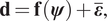 $$ \mathbf{d}=\mathbf{f}\left(\boldsymbol{\psi} \right)+\overline{\boldsymbol{\varepsilon}}, $$
where  $ \overline{\boldsymbol{\varepsilon}} $ represents the measurement or observational noise. We assume that this noise is distributed so that
 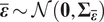 $ \overline{\boldsymbol{\varepsilon}}\sim \mathcal{N}\left(\mathbf{0},{\boldsymbol{\Sigma}}_{\overline{\boldsymbol{\varepsilon}}}\right) $, where
  $ {\boldsymbol{\Sigma}}_{\overline{\boldsymbol{\varepsilon}}}\in {\mathrm{\mathbb{R}}}^{s\times s} $ is a symmetric-positive definite covariance matrix.
The aim in material model calibration is to estimate the posterior distribution of the model parameters, that is the distribution of parameters  $ \boldsymbol{\psi} $ given the observed experimental data. Under the assumption that
  $ \boldsymbol{\psi} $ and
  $ \overline{\boldsymbol{\varepsilon}} $ are independent random variables, Baye’s theorem gives:
 $$ \pi \left(\boldsymbol{\psi} |\mathbf{d}\right):= \frac{1}{Z}\pi \left(\mathbf{d}|\boldsymbol{\psi} \right){\pi}_0\left(\boldsymbol{\psi} \right)\hskip1.1em \mathrm{such}\ \mathrm{that}\hskip1.1em Z:= {\int}_{\boldsymbol{\unicode{x03C8}}}\pi \left(\mathbf{d}|\boldsymbol{\psi} \right){\pi}_0\left(\boldsymbol{\psi} \right)d\boldsymbol{\psi} . $$
The conditional distribution  $ \pi \left(\mathbf{d}|\boldsymbol{\psi} \right) $ defines the likelihood, that is the probability of observing the data
  $ d $ given a set of material parameters
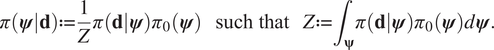
  $ \boldsymbol{\psi} $. Having define the statistical model (1), it follows that:
 $$ \log \pi \left(\mathbf{d}|\boldsymbol{\psi} \right)=\frac{1}{2}{\left(\mathbf{d}-\mathbf{f}\left(\boldsymbol{\psi} \right)\right)}^T{\boldsymbol{\Sigma}}_{{\overline{\boldsymbol{\varepsilon}}}^{-1}}\left(\mathbf{d}-\mathbf{f}\left(\boldsymbol{\psi} \right)\right). $$
 In this setting, we have a classic Bayesian inverse problem for which there are well-established methods in computational statistics for solving. Having said this, the estimation of the posterior distribution of model parameters, even for a single experiment, can be extremely challenging. This is particularly the case when: (a) the evaluation of the parameters-to-observable map  $ \mathbf{f}\left(\boldsymbol{\psi} \right) $ are computationally expensive, (e.g., a nonlinear finite element model); (b) the material parameter space is high-dimensional (i.e.,
  $ m $ is large); or (c) the posterior density has a complex geometry, for example, when multiple parameters have complex nonlinear dependencies. In this article, we use MCMC methods to perform the Bayesian computations and therefore briefly set out the detail here, but they are widely covered in the literature (Liu, Reference Liu2008; Gelman et al., Reference Gelman, Carlin, Stern, Dunson, Vehtari and Rubin2013).
In this contribution, we focus on Metropolis-Hasting-based MCMC algorithms (Roberts and Rosenthal, Reference Roberts and Rosenthal2009), where we generate a chain of  $ n $ samples
  $ \mathcal{T}:= \left\{{\boldsymbol{\psi}}^{(1)},{\boldsymbol{\psi}}^{(2)},\dots, {\boldsymbol{\psi}}^{(n)}\right\} $ of statistically dependent sets of parameters. The chain is produced from a current state
  $ {\boldsymbol{\psi}}^{(i)} $, by making a proposal
  $ {\boldsymbol{\psi}}^{\prime } $ generated from a known proposal distribution
  $ q\left({\boldsymbol{\psi}}^{\prime }|{\boldsymbol{\psi}}^{(i)}\right) $ (Roberts, Reference Roberts2011). This new proposal is accepted as the next state in the chain, that is
  $ {\boldsymbol{\psi}}^{\left(i+1\right)}={\boldsymbol{\psi}}^{\prime } $ with a probability:
 $$ \alpha \left({\boldsymbol{\psi}}^{\prime }|{\boldsymbol{\psi}}^{(i)}\right)=\min \left(1,\frac{\pi \left(\mathbf{d}|{\boldsymbol{\psi}}^{\prime}\right){\pi}_0\left({\boldsymbol{\psi}}^{\prime}\right)q\left({\boldsymbol{\psi}}^{\prime }|{\boldsymbol{\psi}}^{(i)}\right)}{\pi \left(\mathbf{d}|{\boldsymbol{\psi}}^{(i)}\right){\pi}_0\left({\boldsymbol{\psi}}^{(i)}\right)q\left({\boldsymbol{\psi}}^{(i)}|{\boldsymbol{\psi}}^{\prime}\right)}\right), $$
otherwise it is rejected, and  $ {\boldsymbol{\psi}}^{\left(i+1\right)}={\boldsymbol{\psi}}^{(i)} $. The distribution of the complete chain
  $ \mathcal{T} $ converges to the desired posterior
  $ \pi \left(\boldsymbol{\psi} |d\right) $. Although converge can be slow, computations are independent of estimating the normalizing constant
  $ Z $. In particular, the proposal distributions
  $ q\left(\cdot |\cdot \right) $ can be carefully designed to be scalable in high-dimensional parameters spaces, and asymptotically provide an exact (free from bias) approximation of the posterior.
Once a Markov chain  $ \mathcal{T} $ is generated, the expectations of a function
  $ h\left(\boldsymbol{\psi} \right) $ can be estimated by Monte Carlo integration:
 $$ {\unicode{x1D53C}}_{\pi \left(\boldsymbol{\psi} |\mathbf{d}\right)}(h)={\int}_{\boldsymbol{\unicode{x03C8}}}h\left(\boldsymbol{\psi} \right)\;\pi \left(\boldsymbol{\psi} |\mathbf{d}\right)\;d\boldsymbol{\psi} \approx \hat{h}:= \frac{1}{n}\sum \limits_{i=1}^nh\left({\boldsymbol{\psi}}^{(i)}\right). $$
 The computed value  $ \hat{h} $ is an unbiased estimate for the expectation of
  $ h\left(\boldsymbol{\psi} \right) $ under the posterior distribution, and has a mean square error of:
 $$ \unicode{x1D54D}\left(\hat{h}\right)=\frac{\unicode{x1D54D}(h)}{\hskip0.1em ESS\hskip0.1em (h)}=\frac{2\unicode{x1D54D}(h)\tau (h)}{n}, $$
where  $ \tau (h) $ is the integrated autocorrelation of
  $ h\left(\boldsymbol{\psi} \right) $. The function
  $ \hskip0.1em ESS\hskip0.1em (h) $ is the effective samples size of the chain, and gives the approximate number of independent samples from the set of correlated samples generated by a Markov chain, and
  $ \unicode{x1D54D}(.) $ represents the variance of distribution, following the notation in (Kong, Reference Kong1992) and (Kong et al., Reference Kong, Liu and Wong1994).
2.2. Hierarchical Bayesian calibration of a material model from a set of experiments
In practice, engineers are seldom interested in finding the material parameters which best fit a single experimental test, but rather in inferring the population distribution of the parameters given a complete experimental dataset. Let us assume  $ J $ independent experimental tests are performed, which gives the complete dataset:
 $$ \mathcal{D}:= \left\{{\mathbf{d}}^{(1)},{\mathbf{d}}^{(2)}\dots, {\mathbf{d}}^{(J)}\right\}. $$
 Here,  $ {\mathbf{d}}^{\left(, j\right)}\in {\mathrm{\mathbb{R}}}^{s_j} $ denotes the vector of data for the jth experiment. As for the single experimental formulation, we introduce the parameter-to-observable map for each experimental test
  $ {\mathrm{\mathcal{F}}}_j\left(\boldsymbol{\psi} \right):\boldsymbol{\Psi} \to {\mathrm{\mathbb{R}}}^{s_j} $. We note, in particular, that in the formulation which follows, there is no requirement that the experimental tests are the same, this is demonstrated in a computational example (Section 3.2).
We formulate our problem as a HBM (Gelman et al., Reference Gelman, Carlin, Stern, Dunson, Vehtari and Rubin2013; Wolfgang, Reference Wolfgang2016). For each of the  $ J $ experiments, each experiment has its own data
  $ {\mathbf{d}}^{\left(, j\right)} $, and if a single Bayesian calibration was performed (as described above), each could generate its own posterior distribution of material parameters, that is
  $ \pi \left({\boldsymbol{\psi}}^{\left(, j\right)}|{\mathbf{d}}^{\left(, j\right)}\right) $. Such an approach neglects the connection between each experiment that they are different experiments on the same material. It is therefore natural to view each
  $ {\boldsymbol{\psi}}^{\left(, j\right)} $ as a sample from some population distribution. We therefore define a statistical model for the population distribution, parameterized by additional parameters
  $ \boldsymbol{\phi} \in {\mathrm{\mathbb{R}}}^S $. In a hierarchical Bayesian setting, these are referred as hyper-parameters, and in a Bayesian setting, are themselves uncertain and equipped with their own prior densities
  $ \pi \left(\boldsymbol{\phi} \right) $, termed as hyper-priors.
The Bayesian task is, therefore, not to directly infer the distribution of model parameters for each experiment ( $ {\boldsymbol{\psi}}_j $), but rather the distribution of hyper-parameter
  $ \boldsymbol{\phi} $ given our complete set of data
  $ \mathcal{D} $, that is to compute samples from
  $ \pi \left(\boldsymbol{\phi} |\mathcal{D}\right) $. Assuming that each experiment is independent it follows that:
 $$ \pi \left(\boldsymbol{\phi} |\mathcal{D}\right)=\prod \limits_{j=1}^J\pi \left(\boldsymbol{\phi} |{\mathbf{d}}^{\left(, j\right)}\right)=\prod \limits_{j=1}^J{\int}_{\boldsymbol{\Psi}}\pi \left(\boldsymbol{\phi}, \boldsymbol{\psi} |{\mathbf{d}}^{\left(, j\right)}\right)d\boldsymbol{\psi} \propto \prod \limits_{j=1}^J{\int}_{\boldsymbol{\Psi}}\pi \left({\mathbf{d}}^{\left(, j\right)}|\boldsymbol{\phi}, \boldsymbol{\psi} \right)\pi \left(\boldsymbol{\phi}, \boldsymbol{\psi} \right)d\boldsymbol{\psi} . $$
For each experiment, we note that the likelihood  $ \pi \left({\mathbf{d}}^{\left(, j\right)}|\boldsymbol{\phi}, \boldsymbol{\psi} \right) $ is not directly dependent on
  $ \boldsymbol{\phi} $, and hence the dependency is dropped:
  $ \pi \left(\boldsymbol{\psi} |{\mathbf{d}}^{\left(, j\right)}\right) $. The connection between model parameters
  $ \boldsymbol{\psi} $ and hyper-parameters
  $ \boldsymbol{\phi} $ is therefore through their joint distribution
  $ \pi \left(\boldsymbol{\phi}, \boldsymbol{\psi} \right)=\pi \left(\boldsymbol{\psi} |\boldsymbol{\phi} \right)\pi \left(\boldsymbol{\phi} \right) $. It hence follows that:
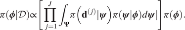 $$ \pi \left(\boldsymbol{\phi} |\mathcal{D}\right)\propto \left[\prod \limits_{j=1}^J{\int}_{\boldsymbol{\Psi}}\pi \left({\mathbf{d}}^{\left(, j\right)}|\boldsymbol{\psi} \right)\pi (\boldsymbol{\psi} |\boldsymbol{\phi} \Big)d\boldsymbol{\psi} \right]\pi \left(\boldsymbol{\phi} \right). $$
If the expression (9) is compared to Baye’s formulae, we therefore identify:
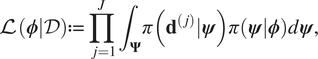 $$ \mathrm{\mathcal{L}}\left(\boldsymbol{\phi} |\mathcal{D}\right):= \prod \limits_{j=1}^J{\int}_{\boldsymbol{\Psi}}\pi \left({\mathbf{d}}^{\left(, j\right)}|\boldsymbol{\psi} \right)\pi \left(\boldsymbol{\psi} |\boldsymbol{\phi} \right)d\boldsymbol{\psi}, $$
as being proportional to the likelihood. This is then an integrated likelihood, which marginalizes out model parameters  $ \boldsymbol{\psi} $. We can therefore proceed with an MCMC calculation in the space of hyper-parameters
  $ \boldsymbol{\phi} $, replacing the likelihood directly with
  $ \mathrm{\mathcal{L}} $.
For all but the simplest of models, the likelihood within (9) cannot be analytically calculated, and hence must be approximated. On the face of it, this looks like an extremely expensive task since, in general, for each of the examples considered in this article, the evaluation of likelihood for an experiment  $ \pi \left({\mathbf{d}}^{\left(, j\right)}|\boldsymbol{\psi} \right) $ is computationally expensive (a nonlinear finite element model) and the number of experiments
  $ J $ maybe large. Yet, a key observation is that the expensive part of the calculation, the evaluation of
  $ \pi \left({\mathbf{d}}^{\left(, j\right)}|\boldsymbol{\psi} \right) $, is independent of
  $ \boldsymbol{\phi} $. The component dependent on
  $ \boldsymbol{\phi} $,
  $ \pi \left(\boldsymbol{\psi} |\boldsymbol{\phi} \right) $, is analytical evaluation of a density (in our examples, a multivariant Gaussian). Therefore, strategies to approximate
  $ \pi \left({\mathbf{d}}^{\left(, j\right)}|\boldsymbol{\psi} \right) $ can be done prior to any sample of the hyper-parameters in an “offline” step.
There are various approaches to approximate the integral  $ \mathrm{\mathcal{L}} $, and which is optimal will be problem dependent. In the examples considered in this article, we choose (before sampling) to build a Gaussian process (GP) emulator to replace the expensive mapping
  $ \boldsymbol{\psi} \to \pi \left({\boldsymbol{d}}^{\boldsymbol{j}}|\boldsymbol{\psi} \right) $. The approximation of likelihood using statistical emulators is described by (Rasmussen, Reference Rasmussen2003), see also (Fielding et al., Reference Fielding, Nott and Liong2011). As is done this contribution, the emulator of the likelihood is trained on a set of space-filling samples from the input space. Although not considered here, it is possible to consider an additional step, whereby a MCMC computation with a specific accept–reject step is carried out to improve the likelihood estimation, by ensuring samples come from the posterior distribution. Where a prior/initial parameter range is poorly specified, it is easy to see this could have a big effect of the quality of the emulator of likelihood, particularly in the case where very sparse evaluations of the model are possible due to computational constraints. This additional step in the article has not being consider, since via cross-validation, the quality of the approximations of the likelihood seem sufficient. However, this additional step could be readily added to the computational pipeline, with no methodological effect of the results presented in this contribution.
Since we have an emulator precomputed for  $ \pi \left({\boldsymbol{d}}^{\boldsymbol{j}}|\boldsymbol{\psi} \right) $, it is natural to use Bayesian quadrature for the marginalization integrals in (10). Bayesian quadrature (Paleyes et al., Reference Paleyes, Pullin, Mahsereci, Lawrence and González2019) gives a mean (
 $ {\mu}_{\mathrm{\mathcal{L}}} $) and standard deviation (
 $ {s}_{\mathrm{\mathcal{L}}} $) for integral
  $ \mathrm{\mathcal{L}}\left(\boldsymbol{\phi} \right) $. For the MCMC step (in the hyperparameter space), a sample
  $ \mathrm{\mathcal{L}}={\mu}_{\mathrm{\mathcal{L}}}+{s}_{\mathrm{\mathcal{L}}}\omega $ where
  $ \omega \sim \mathcal{N}\left(0,1\right) $, can be drawn. By doing so, the MCMC traces will also account for the uncertainty in the approximation of (10). Details of Bayesian Quadrature implemented in this article can be provided in classic contribution (O’Hagan, Reference O’Hagan1991). Since also a Monte Carlo approximation can be used, without any changes to the computational framework presented, the Bayesian Quadrature step is not central to the core idea of this contribution, and we do not provided further details.
3. Demonstrative Examples
In this section, we demonstrate the hierarchical Bayesian framework set out with two computational examples. The first is a simple model for the calibration of an elastic spring, the second is an elastoplastic model for 3D-printed steel using real experimental data.
3.1. Example 1: spring model
In this first example, we consider a simple toy model to demonstrate the methodology presented before considering a much more computational intensive example in Section 3.2 based on a nonlinear finite element model. In this case,we wish to calibrate a simple linear Hookes law model for the load response of the springs under deformation. Due to the manufacturing process, material variability, and measurement uncertainty, the springs display a distribution of responses. To understand the resulting distribution of model parameter, the behavior of  $ N $ independent springs are tested by compressing each spring by an increasing displacement
  $ {x}_i $ and the force
  $ {y}_i $ for
  $ i=1,\dots, M $ to achieve each displacement, which is recorded. From these experiments, we obtain the complete set of data:
 $$ \mathcal{D}:= \left\{{\mathbf{d}}^{(1)},\dots, {\mathbf{d}}^{(N)}\right\}\hskip1.1em \mathrm{where}\hskip1.1em {\mathbf{d}}^{\left(, j\right)}\in {\mathrm{\mathbb{R}}}^M. $$
In this example, the data are generated synthetically, by the (nonlinear) spring model given by:
 $$ {f}_i^{\left(, j\right)}={c}_1{x}_i+{c}_2{x}_i^{\alpha }+\overline{\varepsilon},\hskip1.1em \mathrm{so}\hskip0.3em \mathrm{that}\hskip1.1em {\mathbf{d}}^{\left(, j\right)}={\left[{f}_1^{\left(, j\right)},\dots, {f}_M^{\left(, j\right)}\right]}^T, $$
where 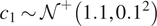 $ {c}_1\sim {\mathcal{N}}^{+}\left({\mathrm{1.1,0.1}}^2\right) $,
 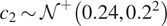 $ {c}_2\sim {\mathcal{N}}^{+}\left({\mathrm{0.24,0.2}}^2\right) $,
 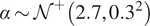 $ \alpha \sim {\mathcal{N}}^{+}\left({\mathrm{2.7,0.3}}^2\right) $,
  $ \overline{\varepsilon}\sim \mathcal{N}\left({\mathrm{0,0.02}}^2\right) $, where
  $ {\mathcal{N}}^{+}\left(.,.\right) $ denotes a truncated normal distribution. The control points
  $ {x}_i $ are taken to be
  $ M=5 $ equally spaced displacements between
  $ {x}_1=0 $ and
  $ {x}_5=0.5 $, and synthetic data were generated for
  $ J=10 $ experiments.
We assume the parameter-to-observable map is taken to be a linear mathematical relationship between force and displacement (Hooke’s Law), and is the same for each experiment  $ j=1,\dots, J $:
 $$ f\left(x,k\right)= kx,\hskip1.1em \mathrm{where}\hskip1.1em k\in {\mathrm{\mathbb{R}}}^{+}. $$
 For each experiment, the misfit between model and data points are assumed to be independent, isotropic, Gaussian with zero mean and unknown variance  $ {s}^2 $, that is as defined by (3) with
  $ {\Sigma}_{\varepsilon }={s}^2\unicode{x1D540}\in {\mathrm{\mathbb{R}}}^{4\times 4} $ with
  $ {\Sigma}_{\overline{\varepsilon}}={s}^2\unicode{x1D540}\in {\mathrm{\mathbb{R}}}^{5\times 5} $. This captures the measurement uncertainty (generated by
  $ \overline{\varepsilon} $ in (12)) and in this case, the model misspecification here is that the data are actually generated from a nonlinear model (12). The uncertain parameters for each experiment are therefore wrapped into a vector
  $ \boldsymbol{\psi} ={\left[k,s\right]}^T $.
The problem can now be formulated into the hierarchical Bayesian setting, and therefore, hyper-parameters which describe the population statistics of  $ k $ and
  $ s $ are introduced:
 $$ k\sim {\mathcal{N}}^{+}\left({\mu}_k,{v}_k\right)\hskip1.1em \mathrm{and}\hskip1.1em s\sim {\mathcal{N}}^{+}\left({\mu}_s,{v}_s\right). $$
 This gives four hyper-parameters, which are collected into a single vector  $ \boldsymbol{\phi} ={\left[{\mu}_k,{v}_k,{\mu}_s,{v}_s\right]}^T $. Finally, hyper-priors are defined for each component of
  $ \boldsymbol{\phi} $, such that:
 $$ {\displaystyle \begin{array}{l}\hskip2.28em {\mu}_k\sim {\mathcal{N}}^{+}\left(\mathrm{1.0,0.1}\right),\hskip1em {v}_k\sim {\mathcal{N}}^{+}\left(\mathrm{0.3,0.1}\right),\\ {}\hskip1em {\mu}_s\sim {\mathcal{N}}^{+}\left(\mathrm{0.3,0.1}\right)\hskip1.1em \mathrm{and}\hskip1.1em {v}_s\sim {\mathcal{N}}^{+}\left(\mathrm{0.03,0.01}\right).\end{array}} $$
 The next step is to build  $ J=10 $ independent GPs, for the mapping between
  $ \psi \to \pi \left(\psi |{\mathbf{d}}_j\right) $, for
  $ j=1,\dots, J $. GPs were trained using the open source package GPy (GPy, 2012). After some initial testing, an ARD
  $ 5/2 $ Matérn kernel with a zero mean function was chosen to define each GP emulator. The kernel is defined by the two-point correlations function:
 $$ c\left(\boldsymbol{\psi}, {\boldsymbol{\psi}}^{\prime}\right)=\frac{\sigma_r^2d{\left(\boldsymbol{\psi}, {\boldsymbol{\psi}}^{\prime}\right)}^{5/2}}{\Gamma \left({\nu}_k\right){2}^{5/2}}{K}_{5/2}\left(d\left(\boldsymbol{\psi}, {\boldsymbol{\psi}}^{\prime}\right)\right)\hskip1.1em \mathrm{where}\hskip1.1em d\left(\boldsymbol{\psi}, {\boldsymbol{\psi}}^{\prime}\right):= \sqrt{5\sum \limits_i^2{\left(\frac{{\boldsymbol{\psi}}_i-{\boldsymbol{\psi}}_i^{\prime }}{{\mathrm{\ell}}_i}\right)}^2}, $$
where  $ {K}_{5/2}\left(\cdot \right) $ is a modified Bessel function and
  $ \Gamma \left(\cdot \right) $ is the gamma function. The additional hyper-parameters for the Matérn covariance
  $ {\sigma}_r^2 $, the variance and
  $ \mathrm{\ell}=\left[{\mathrm{\ell}}_1,{\mathrm{\ell}}_2\right] $, the characteristic length scale, are free-parameters that are optimized during the training process. To train each model, we consider
  $ 100 $ samples drawn using a Latin Hypercube (SMT2019, 2019), a quasi-random (space-filling) sampler. Given initial starting points for the hyper-parameters of the Matérn kernel (15), the parameters are optimized to maximize the log-likelihood over the complete dataset using GPy’s default optimizer L-BFGS-B (GPy, 2012; Paleyes et al., Reference Paleyes, Pullin, Mahsereci, Lawrence and González2019).
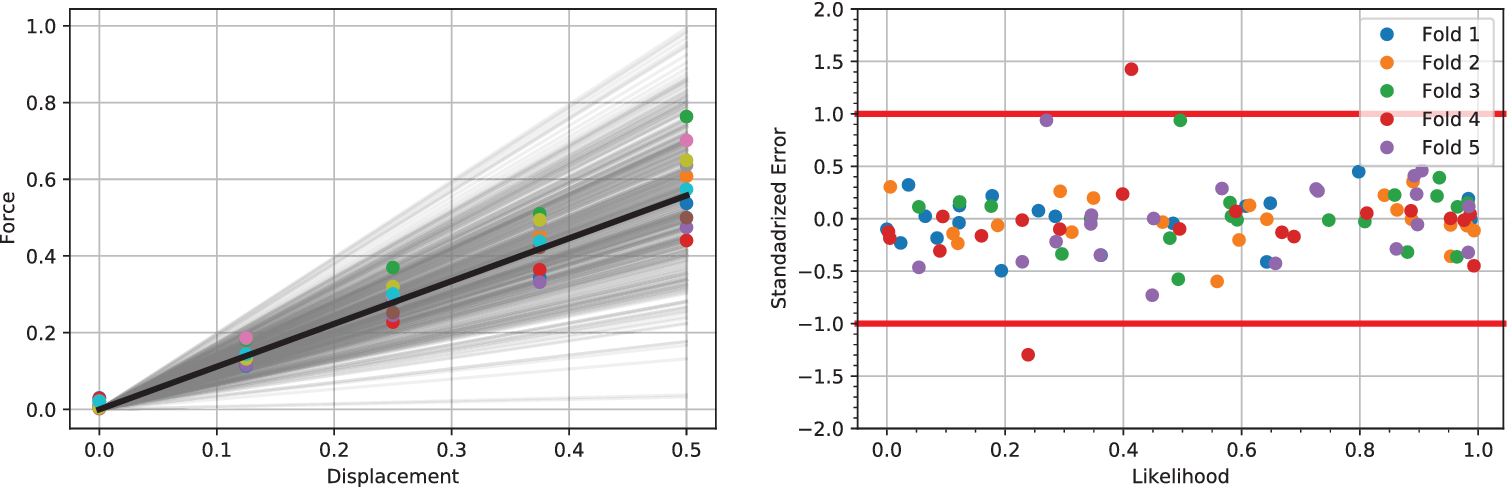
To test the resulting emulators, we perform a fivefold cross-validation test. The 100 training points are divided into five groups. The GP is trained with four groups and last group is used for the test, the process is repeated five times assigning a different “test group” each time. In each case, we consider the individual standardized errors for  $ j=1,\dots, 20 $ left out samples defined by:
 $$ {e}_j=\frac{f\left({x}_j\right)-{m}^{\ast}\left({x}_j\right)}{\sqrt{v^{\ast}\left({x}_j,{x}_j\right)}}, $$
where  $ f\left({x}_j\right) $ is the value of the actual model,
  $ {m}^{\ast}\left({x}_j\right) $,
  $ {v}^{\ast}\left({x}_j,{x}_j\right) $ is the value of the mean and covariance function of our GP at
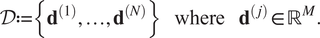
  $ {x}_j $. Figure 2 (right) shows the standardized error for 20 points along with lines of one standard deviation. As it is assumed that the noise error follows a normal distribution
  $ \mathcal{N}\left(0,1\right) $ along with the natural uncertainty, we expect the standardized error to follow the same normal distribution and that no more than two points of each fold falls outside of the standard deviation line. This derives from the fact that we target in a 90% confidence interval (CI) which is a well-trained emulator. In every subfigure, each different fold is marked with a different color (and shape), so overall, we conclude that the emulators are well-trained as no more than two points of the same color (shape) are outside of the bounds in any figure.
(Left) Five hundred samples from the full posterior of  $ f= kx $ alongside experimental data points for
  $ J=10 $. The mean of all posterior samples is plotted in as a solid black line. (Right) Shows the validation of a single experiment and associated Gaussian process using a fivefold analysis. Results demonstrate a well-trained model, since in the five folds only a single point has a standard error of magnitude greater 1. Similar good validation results are observed for all
  $ 10 $ experiments.
Following the HBM setup in Section 2.2, a Metropolis-Hastings algorithm driven by precondition Crank–Nicolson (pCN) proposal distribution including a simple adaptive scaling was used (Cotter et al., Reference Cotter, Roberts, Andrew and White2013). A single MCMC of 25,000 samples was computed with a target acceptance rate of  $ 25\% $. The first 5,000 samples were discarded for burn-in. The effective sample size for each of the hyper-parameters was computed such that
 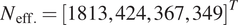 $ {N}_{\mathrm{eff}.}={\left[\mathrm{1813,424,367,349}\right]}^T $ giving sampling error
  $ {S}_{err}=\left[\mathrm{0.090,0.021,0.018,0.017}\right] $, for
  $ {\mu}_{\psi } $,
  $ {v}_{\psi } $,
  $ {\mu}_s $,
  $ {v}_s $, respectively. The sampling errors are sufficiently small relative to the quantities estimated, and hence the number of effective samples in each case are deemed sufficient. Figure 3 shows the traces and the posterior distribution of all hyper-parameters considering 10 independent data. The effective sample sizes for each parameter could be improved using more sophisticated sampling methods, for example Hamiltonian Monte Carlo (Duane et al., Reference Duane, Kennedy, Pendleton and Roweth1987) or more refined adaptive Metropolis sampler (Haario et al., Reference Haario, Saksman and Tamminen2001).
(Top Row) Traces for the four hyper-parameters  $ {\mu}_k $,
  $ {v}_k $,
  $ {\mu}_s $, and
  $ {v}_s $. (Bottom Row) Posterior distributions of the hyper-parameters (left)
  $ {\mu}_k $ and
  $ {v}_k $ and (right)
  $ {\mu}_s $ and
  $ {v}_s $ of the hyper-parameters.
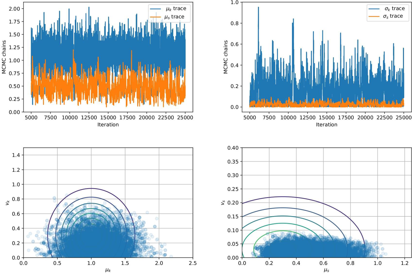
We observe from Figure 3 that the posterior samples are strongly influenced by the data, demonstrated by the qualitative difference between prior and posterior distributions. This is expected since the synthetic data are generated from a nonlinear spring model, and the statistical model accounts for model misspecification and measurement uncertainty within a single parameter  $ s $. In particular, we observe an expected value
  $ {\mu}_k=1.17 $, higher than the prior value specified (
 $ {\mu}_k=1 $), but closer to the value used to generate the data
  $ {\mu}_k=1.1 $ mean value of
  $ {c}_1 $ (
 $ {\mu}_{c_1}=1.1 $). For real-world problems, additional work could be done to better specify a statistical model for the model missspecification, accounting for the fact there is greater model mismatch at larger strain values, and/or impose a more informed prior. However, this is outside the scope of this article for a simple demonstrative example.
In testing, MCMC simulations were repeated with increasing amounts of experimental data, so that in total, we have results for 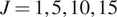 $ J=\mathrm{1,5,10,15} $, and
  $ 20 $. In each case, posterior chains were thinned using estimated auto-correlation lengths to achieve approximately independent samples for statistical analysis. For each group of experiments, descriptive statistics for each chain were computed and are summarized in Table 1. We analyze the convergence of posterior distribution under increasing number of experiments by estimating the Kullback–Leibler (KL) divergence (Kullback and Leibler, Reference Kullback and Leibler1951), comparing the posterior distributions as new data. In the table, the KL divergence as the number of experiments are incremented are denoted
  $ {\Delta}_{KL} $. The results in the Table 1, in particular, the decreasing KL divergence between sequential distributions, and Figure 4 (left) shows the convergence of the distribution with increasing number of experiments as expected. With the exception of the case
  $ J=1 $, we observe a reduction in uncertainty (decrease in estimated variance) as we increase the amount of data. This corresponds to the reduction in the sampling error of the experimental data, allowing us to better represent the population statistics. A plot of a random 500 realization from the posterior for
  $ J=10 $, alongside the original experimental data is shown in Fig.4 (right). All samples bound the experimental results, while the mean of the posterior samples provides a qualitatively sensible estimate for all the experiments.
Descriptive statistics of posterior samples for an increasing number of experimental tests  $ J $
$ J $

Kullback–Leibler (KL) divergence  $ {\Delta}_{KL} $ is approximated between distribution as each set of data is added.
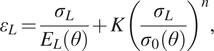
(Left) Shows the distribution of  $ k\sim {N}^{+}\left(\unicode{x1D53C}\left[{\mu}_k\right],\unicode{x1D53C}{\left[{v}_k\right]}^2\right) $ for increasing amounts of data
  $ J=1,\dots 20 $. (Right) This figure shows the difference between the two distributions, the first which is denoted with “point marker” comes for
 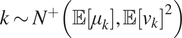 $ k\sim {N}^{+}\left(\unicode{x1D53C}\left[{\mu}_k\right],\unicode{x1D53C}{\left[{v}_k\right]}^2\right) $ while the other (denoted with “dash-dot line”) is a maximum entropy approximated (with four moments matched) constructed from all posterior samples.
Before considering an example with real experimental data, we apply the maximum entropy approximation of all posterior samples. A maximum entropy approximation for  $ k $ was obtained with a four-moment representation of the distribution to all posterior samples. The results are shown in four (right), in which the maximum entropy approximation of the full posterior (dash-dot line) is plotted alongside the mean estimate
  $ k\sim N\left(\unicode{x1D53C}\left[{\mu}_k\right],\unicode{x1D53C}{\left[{v}_k\right]}^2\right) $ (dot line). As expected, we see that full posterior distribution has greater uncertainty. This captures the effects of approximating population distributions with only a finite number of experiments, but also the uncertainty imposed by the assumption that the population distribution is Gaussian. The maximum entropy calculations allow the posterior distribution to be efficiently represented (here with just four numbers) rather than many thousands of samples, thereby simplifying the stochastic computational pipeline in a sequence of engineering calculations.
3.2. Example 2: stochastic elastoplastic model for 3D-printed steel
In this section, our approach is applied to a real experimental dataset provided by coupon tests of 3D-printed steel (Gardner et al., Reference Gardner, Kyvelou, Herbert and Buchanan2020). The study extends a previous Bayesian study for estimating uncertain material parameters using these data, as described in Dodwell et al. (Reference Dodwell, Fleming, Buchanan, Kyvelou, Detommaso, Gosling, Scheichl, Gardner, Girolami and Oates2021). In the previous study, a standard Bayesian approach was presented, whereby all experiments were fitted with single values of parameters rather than population distribution as developed in the HBM. This section provides a brief overview of the engineering context, the mathematical and stastistical model setup and focuses on the results using our presented approach.
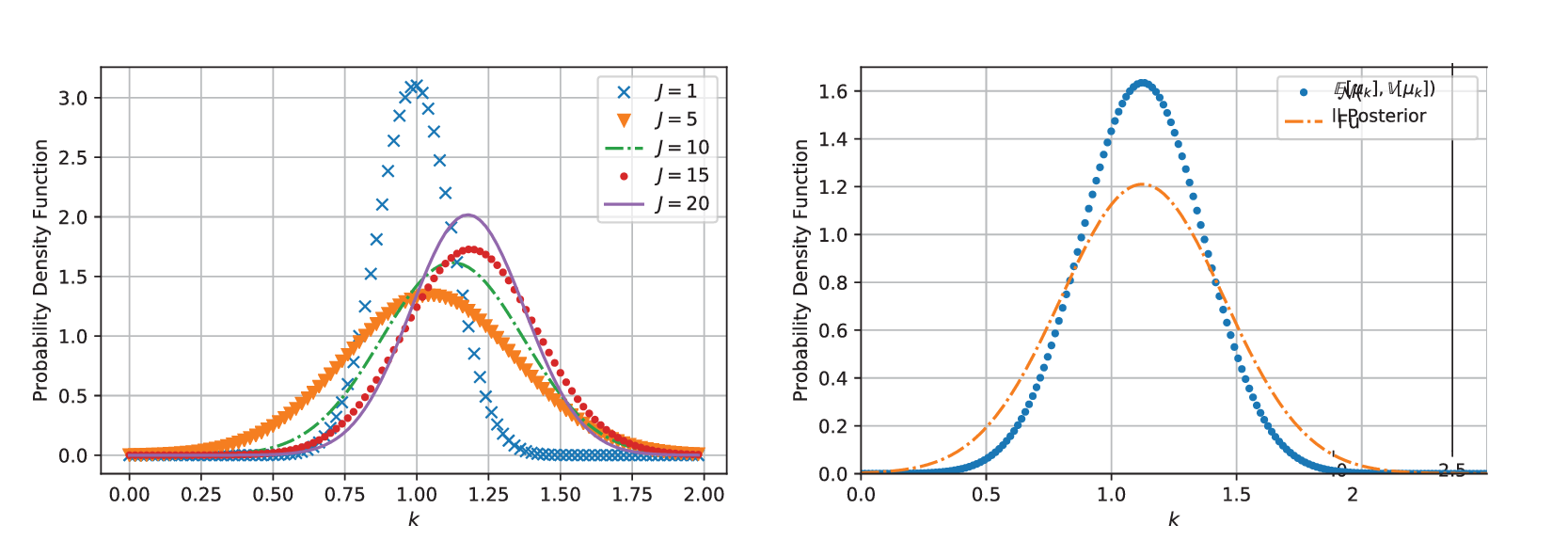
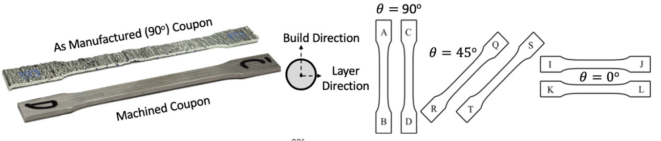
Additive manufacturing (AM) technologies are developing at a rapid pace, enabling the manufacture of advanced components with near arbitrary complexity. Various techniques have been developed for metallic AM including powder bed fusion and direct energy deposition. An interesting class of direct energy deposition are wire arc additive manufacturing (or WAAM), a process using a robotic arm and an arc welding tool (Figure 5, left). This novel technology can build large scale structures in situ, at relatively high deposition rates ( $ \sim 4 $ kg/h). A well-documented example is the pedestrian bridge developed by Dutch startup MX3D (Figure 5, right). The complexity of possible parts along the uncertain thermal deformations of the material during welding, means that the as-manufactured material properties of WAAM are uncertain. In this section, we apply our hierarchical Bayesian approach to calibrate a stochastic elastoplastic model for WAAM.
(Left) The 3D-printing protocol developed by MX3D uses a weld head attached to a robotic arm (image by Joris Laarman, www.jorislaarman.com). (Middle) Pedestrian bridge manufactured using 3D-printed steel (7). (Right) Test set of up of individual coupons.
The dataset reported by Gardner et al. (Reference Gardner, Kyvelou, Herbert and Buchanan2020) are a set of six smoothed/machined tensile coupons, manufactured and tested according to the EN ISO 6892-1 standard (ISO, 2019), see Figure 6. The coupons were cut at angles  $ \psi ={0}^{\circ } $, 45
 $ {}^{\circ } $ and 90
 $ {}^{\circ } $ from a single larger WAAM steel plate. Here,
  $ \theta $ is the angle of the layering relative to the build direction as shown in Figure 6. In total, two experiments are performed for each build direction, hence
  $ J=6 $. For each test, the cross-sectional areas
  $ {A}_c $ of each coupon are measured, while the testing machine measures the applied tensile load and a four-camera LaVision digital image correlation system provides averaged surface strain measurements from both sides. Using these measurements, for each of the six experiments, the longitudinal stress
  $ {\sigma}_L $ at eight equally spaced longitudinal strain values
  $ {\varepsilon}_L $ between
  $ 0\% $ and
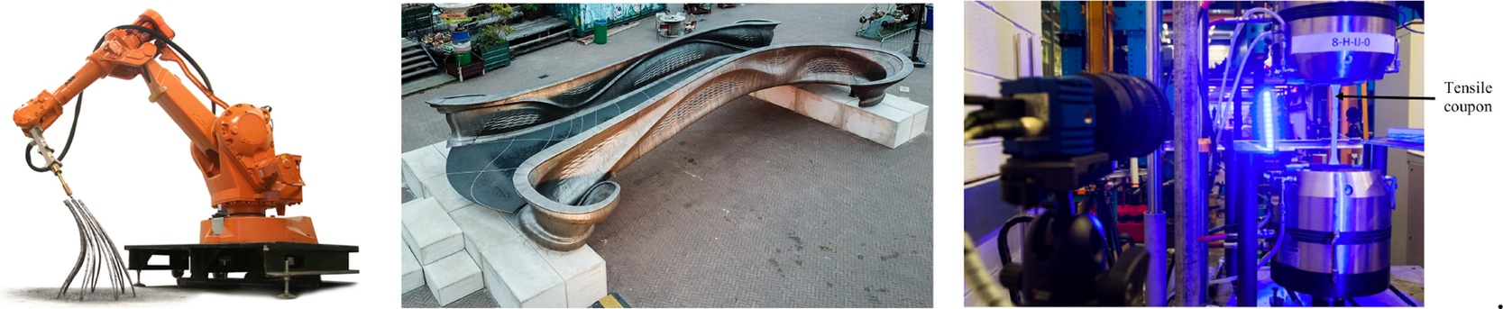
  $ 0.8\% $ is calculated. Each experimental test is modeled using a Ramberg–Osgood model (Ramberg and Osgood, Reference Ramberg and Osgood1943),
 $$ {\varepsilon}_L=\frac{\sigma_L}{E_L\left(\theta \right)}+K{\left(\frac{\sigma_L}{\sigma_0\left(\theta \right)}\right)}^n, $$
Test coupons were machined to remove influence of geometric surface features and cut at angles  $ \theta ={0}^{\circ } $,
  $ {45}^{\circ } $, and
  $ {90}^{\circ } $ perpendicular to the printing direction (Buchanan et al., Reference Buchanan, Esther and Leroy2018).
where  $ {E}_L\left(\theta \right) $ and
  $ {\sigma}_0\left(\theta \right) $ are the unknown longitudinal elastic modulus and yield strengths, respectively, for a coupon with layers oriented at an angle
  $ \theta $,
  $ n $ is an unknown scalar hardening exponent and
  $ K $ is a constant. In this work,
  $ K $ is equal to 0.002 and, as a consequence, the yield strength
  $ {\sigma}_0 $ corresponds to the
  $ 0.2\% $ proof stress, which is widely used to define the yield of metals in the literature (Gardner et al., Reference Gardner, Kyvelou, Herbert and Buchanan2020).
Collectively, by testing coupons over a range of angles, the Ramberg–Osgood model can be used to define a general anisotropic homogeneous, elastoplastic constitutive law under plane stress conditions over all angles  $ \theta $. In this contribution, the elastic part of the deformation is consider to be transversely isotropic, parameterized by
  $ {E}_1,{E}_2,{G}_{12} $, and
  $ {\nu}_{12} $, respectively the elastic moduli perpendicular and parallel to the build direction, a shear modulus and a Poisson ratio. For the plastic response, Hill’s quadratic yield surface (Hill, Reference Hill1948) is considered which, under plane stress assumptions, is uniquely parameterized by three parameters (
 $ F,G,N $). Post-yield, a simple isotropic hardening rule is defined by the single exponent,
  $ n $. The mathematical connection between the Ramberg–Osgood model and the two-dimensional elastoplastic material parameters is provided in the Appendix. As a result, all experiments are described by a single vector of parameters, such that:
 $$ \boldsymbol{\psi} =\left[{E}_1,{E}_2,{G}_{12},{\nu}_{12},{\sigma}_y\left({0}^{\circ}\right),{\sigma}_y\left({90}^{\circ}\right),{\sigma}_y\left({45}^{\circ}\right),n,{s}_e\right]. $$
 The data for each experiment is represented in a vector  $ {\mathbf{d}}^{\left(, j\right)}\in {\mathrm{\mathbb{R}}}^8 $, which contains the eight evenly spaced strain values. The mapping between parameter values and data are defined by the forward map:
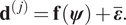 $$ {\mathbf{d}}^{\left(, j\right)}=\mathbf{f}\left(\boldsymbol{\psi} \right)+\overline{\boldsymbol{\varepsilon}}. $$
 Once again,  $ \overline{\boldsymbol{\varepsilon}} $ is a random vector that represents measurement error, whose components are independent and Gaussian with
 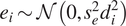 $ {e}_i\sim \mathcal{N}\left(0,{s}_e^2{d}_i^2\right) $, whereby the noise-to-signal parameter
  $ {s}_e $ is to be learned, providing a quantitative measurement of uncertainty in both the data and the model (i.e., as for the first example allowing for model misspecification). For all parameters except
  $ {s}_e $, it is assumed that it comes from a normal distribution, that is
 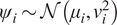 $ {\psi}_i\sim \mathcal{N}\left({\mu}_i,{v}_i^2\right) $, while
  $ {s}_e $ is single value across all experiments. Gathering the mean and variance for each parameter and a single value for
  $ {s}_e $, gives a vector of hyper-parameters of
  $ 17 $ parameters. Each of these is equipment with weakly informed prior distributions, defined by normal distributions over plausible ranges for the parameters given the least mean square fitting reported in (Gardner et al., Reference Gardner, Kyvelou, Herbert and Buchanan2020). All prior values are summarized and given in the Table 2.
Summary statistics of prior and posterior distributions, N—normal and HN—half normal.
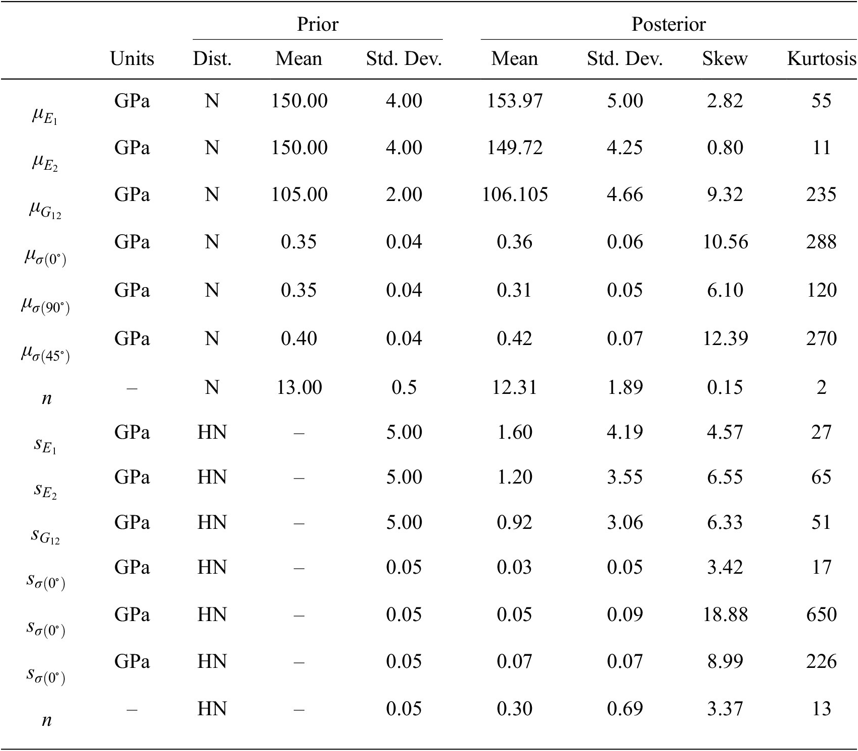
MCMC simulations were carried out as described in Section 2. In this example, since the parameter space is larger than the previous example, a more sophisticated sampling approach is required. Hence all calculations are implemented in PyMC3 (Salvatier et al., Reference Salvatier, Wiecki and Fonnesbeck2016), for which sampling was achieved using the inbuilt sampler DEMetropolizZ, a differential evolution Markov chain methods with embedding snooker updating (Braak and Vrugt, Reference Braak and Vrugt2008). Once again, Gaussian emulators are built for each of the six experiments using GPy, for which a nine-dimensional ARD Matérn covariance (15) is used and trained with  $ 300 $ samples per experiment and using a sixfold cross-validation analysis, very much as described in Example 1. In total, 5,000 samples were computed using MCMC, divided equally between four independent chains. The first 250 samples in each chain were neglected for burn in.
Summary statistics of prior and posterior samples are given in Table 2. For the first example, the distribution of possible observed individual samples can be constructed by sampling the hyper-distributions for hyper-parameters given by the posterior samples. Figure 7 (left) displays such posterior samples showing the possible distribution of stress–strain curves in relation to the experimental data (solid dots), with colors differentiating the build angles  $ \theta ={0}^{\circ } $,
  $ {45}^{\circ } $, and
  $ {90}^{\circ } $. the two polar plots in Figure 7 (middle and right) shows posterior samples (green and red), the maximum a posteriori estimate of longitudinal elastic modulus and proof stress over the sweep of possible build angles
  $ \theta $. Here, isotropic behavior would be observed as a quarter circle (constant radius) for both properties. For both elastic and yield properties, the posterior samples clearly show an uncertain anisotropic material response, as discussed in more detail in Dodwell et al. (Reference Dodwell, Fleming, Buchanan, Kyvelou, Detommaso, Gosling, Scheichl, Gardner, Girolami and Oates2021).
(Left) Samples strain–stress curves via realization of the Ramberg–Osgood model (16). Data points are for two experiments, two for each build angle. (Right) Posterior samples for longitudinal stiffness and proof stress as a function of build angle. Bold lines show maximum a posteriori estimates.
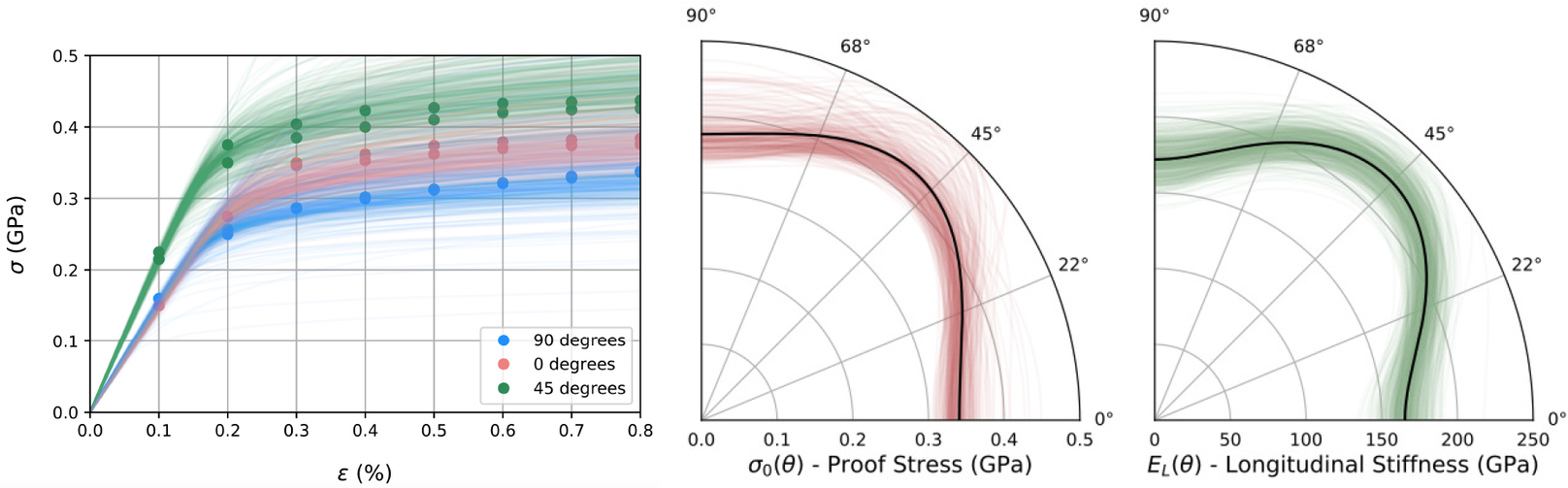
In our hierarchical Bayesian results, even with broad priors for the standard deviations of the population distributions for each parameter, for example  $ {s}_{E_1},{s}_{E_2} $, we observe the posterior variances for the hyper-distributions are relatively small, while the variance of the means are large. This suggests the limited data show good agreement with the low predicted population variances. Qualitatively visualizing the evaluation of posterior samples of our model compares well with the data. However, some parameters in this approach are relatively insensitive to moderate variations in their values. For example, parameter
  $ {E}_1 $ effects only
  $ {0}^{\circ } $ coupons and the initial linear part of the curve (approximately
  $ 1/4 $ of the curve), and is therefore informed by only
  $ 1/12 $ of the data. Therefore, variations in fitting this value has a much smaller effect on the overall likelihood than one might expect.
4. Conclusion
In this article, we develop a formal hierarchical Bayesian methodology for the calibration of parameters of a material model from a set of experiments. The article extends existing probabilistic mechanics literature which previously only considered the calibration specific to a single experiment. When only a single experimental result is used, this may lead to significant bias in the acquired posterior distributions. Clearly, this is because it is a single experimental test is drawn from a population distribution of possible tests, and a result inference from a single experiment will be over-optimistic. Using a formal HBM, we naturally account for the population variation in the experiments with resulting posterior distribution appropriately showing higher variance. This is supported in the test cases, both synthetic and real-world.
The computational challenges which arise for the hierarchical model are significant. Rather than inferring over a single experiment, inference is required over all experiments simultaneously. However, assuming that each experiment is independent, it is possible to marginalize all parameters for a given experiment and formulate the resulting Bayesian calculations in terms of the hyper (population) parameters alone. While this marginalization integral appears computationally expensive, we show that it can be readily approximated using Bayesian quadrature using a precomputed Gaussian emulator as a surrogate to good effect. There might be limitations where the number of material parameters for a model becomes particularly high, but this is not typical in a material model. In such cases, a more crude Monte Carlo approximation would work.
We compute full posterior distributions of hyper parameters using Metropolis Hasting MCMC. Clearly, when there is a large number of experiments and the model and computations are very expensive, then approximate approaches could be taken. For example, likelihoods could be approximated with only random batches of experiments, or clearly approximate Bayesian methods, for example, a Laplace approximation or variational methods could be readily deployed in the same framework.
Funding Statement
This work was funded through TD’s Turing AI Fellowship (2TAFFP/100007).
Data Availability Statement
Data can be obtained by sending a personal e-mail to the contributors, N. Papadimas (np380@exeter.ac.uk) or professor T. Dodwell (T.Dodwell@exeter.ac.uk).
Author Contributions
Conceptualization: N.P. and T.D.; Data curation: N.P. and T.D.; Formal analysis: T.D.; Methodology: N.P. and T.D.; Software: N.P. and T.D.; Supervision: T.D.; Validation: N.P. and T.D.; Writing-original draft: N.P. and T.D.; Writing-review & editing: N.P. and T.D.; Both the authors approved the final submitted draft.
Competing Interests
The authors declare no competing interests exist.
Appendix
Plane-stress elastoplastic model
Consider a coupon which occupies the domain  $ \Omega \in {\mathrm{\mathbb{R}}}^3 $, with global coordinate system
  $ \left(x,y,z\right)\in {\mathrm{\mathbb{R}}}^3 $, alongside a local coordinate system
  $ \left({x}_1,{x}_2,{x}_3\right)\in {\mathrm{\mathbb{R}}}^3 $. Here, the local coordinate
  $ {x}_1 $ is parallel to the layering at an angle
  $ \theta $ to the global
  $ x $ axis,
  $ {x}_2 $ is the build direction and
  $ {x}_3\equiv z $ is normal to the plane of the coupon.
For each experiment with a layer orientation  $ \theta $ to the horizontal axis
  $ x $, the experiments provide longitudinal stress values
  $ {\sigma}_L\equiv {\sigma}_y $ at given values of longitudinal strains
  $ {\varepsilon}_L\equiv {\varepsilon}_y $. The connection from this experimental data to global material parameters/properties is a two-stage process. Each experiment is modeled using a 1D Ramberg–Osgood model
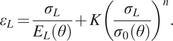 $$ {\varepsilon}_L=\frac{\sigma_L}{E_L\left(\theta \right)}+K{\left(\frac{\sigma_L}{\sigma_0\left(\theta \right)}\right)}^n. $$
 This model is defined by three parameters  $ {E}_L\left(\theta \right) $,
  $ {\sigma}_0\left(\theta \right) $, and
  $ n $, where
  $ K $ is taken to be the fixed constant
  $ 0.02 $. In modeling the overall material, since the
  $ z $ dimension is relatively thin, plane-stress assumptions are imposed. In this section, the connection is set out between the independent Ramberg–Osgood parameters to eight global material parameters, which are made up of four elastic material parameters
  $ {E}_1 $,
  $ {E}_2 $,
  $ {G}_{12} $, and
  $ {\nu}_{12} $, three independent stress factors
  $ F $,
  $ G $, and
  $ N $ which define the onset of yield and a single (
 $ \theta $ independent) hardening parameter,
  $ n $.
The transversely anisotropic elastic properties of the material are defined uniquely by four parameters  $ {E}_1 $,
  $ {E}_2 $,
  $ {G}_{12} $, and
  $ {\nu}_{12} $. The connection between local stresses and strains are defined by the compliance or stiffness matrices, given by
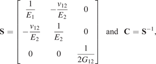 $$ \mathbf{S}\hskip1.5pt =\left[\begin{array}{ccc}\frac{1}{E_1}& -\frac{\nu_{12}}{E_2}& 0\\ {}-\frac{\nu_{12}}{E_2}& \frac{1}{E_2}& 0\\ {}0& 0& \frac{1}{2{G}_{12}}\end{array}\right]\hskip1.1em \mathrm{a}\mathrm{n}\mathrm{d}\hskip1.1em \mathbf{C}\hskip1.5pt =\hskip1.5pt {\mathbf{S}}^{-1}, $$
respectively. Our controlled data from the experiments are measure values of stress in the longitudinal direction  $ {\sigma}_y\equiv {\sigma}_L $ at known longitudinal strain values
  $ {\varepsilon}_y\equiv {\varepsilon}_L $. For the experimental setup, the applied values of
  $ {\sigma}_x $ and
  $ {\tau}_{xy} $ are both zero. The resulting global strains, in global coordinates, can be calculated by rotating local coordinate properties by the layer orientation
  $ \theta $, so that
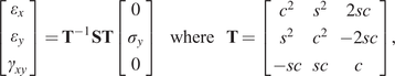 $$ \left[\begin{array}{c}{\varepsilon}_x\\ {}{\varepsilon}_y\\ {}{\gamma}_{xy}\end{array}\right]={\mathbf{T}}^{-1}\mathbf{ST}\left[\begin{array}{c}0\\ {}{\sigma}_y\\ {}0\end{array}\right]\hskip1.1em \mathrm{where}\hskip1.1em \mathbf{T}=\left[\begin{array}{ccc}{c}^2& {s}^2& 2 sc\\ {}{s}^2& {c}^2& -2 sc\\ {}- sc& sc& c\end{array}\right], $$
where  $ c=\cos \left(\theta \right) $ and
  $ s=\sin \left(\theta \right) $. From this relationship, it follows that the elastic stiffness matrix in global coordinates is
  $ \hat{\mathbf{C}}={\hat{\mathbf{S}}}^{-1} $, whereby the longitudinal stiffness (the stiffness connecting longitudinal strains and stresses) is given by the entry
  $ {\hat{\mathbf{C}}}_{22}={E}_L $. This relationship provides a direct-mapping between material parameters
  $ {E}_1 $,
  $ {E}_2 $,
  $ {G}_{12} $, and
  $ {\nu}_{12} $ and the observed/controlled parameters
  $ \theta $ and
  $ {E}_L $. In general, the inverse of this map is ill-posed. However, in our setting data from experiments at multiple angles are available, enabling all parameters to in principle be identified.


 Open access
Comments
No Comments have been published for this article.