Introduction

We consider a polythermal ice mass to consist of several disjointed regions, each exhibiting physically distinct behaviour and peculiar flow properties. Some parts are cold, others are temperate. We define a material particle to be in the cold zone if its temperature is below the local melting point. The definition of temperate ice is less straightforward. In fact, impurities contained in the polycrystalline ice complicate the definition of the pressure-melting point. Here, we ignore these for simplicity and regard the pressure-melting point to be given by the Clausius-Clapeyron equation of pure water. (Reference PatersonPatterson 1981; see also references therein) reviewed the physical properties of temperate ice in more detail and also discussed the origin of moisture in temperate ice. Water flow through glaciers occurs on various scales, from macroscopic channels to intergranular flow through veins with diameters of fractions of millimeters. The permeability of temperate ice itself must therefore be very small, but it is certainly also influenced by the presence of air bubbles and included salts. It will be assumed here that the moisture content is primarily produced by strain heating and thus is relatively small, in contrast to temperate alpine glaciers under warm summer melt conditions, for which a different theoretical model including Darcy’s law is needed.

Reference FowlerFowler (1984) rightly stressed the fact that only internal heat generation may lead to an internal "mushy" zone where two phases of ice and water co-exist. A heat source at a boundary leads merely to the classical Stefan problem of a melting surface. The geothermal heat flux, together with the frictional heat generated at the base and the radiative and turbulent energy fluxes at the free surface, are the relevant surface heat sources and do not per se lead to a temperate ice zone. On the other hand, the strain heating that is primarily effective in the basal ice, the percolation of meltwater in surface firn layers and, to a minor degree also, the radiation penetration in a rather thin surface layer, represent internal volumetric heat sources that are operative in producing temperate ice.

Cold and temperate ice are separated by a surface across which the water content may jump from zero on the cold side to a positive value on the temperate side. In Figure 1, we depict five polythermal structures, the observational evidence of which was summarized by Reference Hutter, Blatter and FunkHutter and others (1988) and references therein. Presumably, the most important type of cold-temperate transition surface (CTS) occurs at or near the base of otherwise cold Arctic and alpine ice masses (Fig. 1d and e). The importance of this feature for the dynamics is obvious: temperate basal ice not only leads to increased shear rate there but also to sliding over the bed, and may thus "destabilize" the ice mass.

Fig. 1. Various types of polythermal structures in glaciers. The shaded areas denote the temperate parts of the ice and the dashed lines along the cold-temperate transitions indicate parts with melting conditions. The arrows indicate the approximate position of the average. equilibrium line.

Polythermal regimes with a temperate basal layer in an otherwise cold glacier are suspected to exist in White Glacier, Axel Heiberg Island (Reference BlatterBlatter, 1987) and Laika Glacier (unofficial name; 75°53’N, 79°10’W; see Fig. 2), Coburg Island (Reference Blatter and KappenbergerBlatter and Kappenberger, 1988), Canadian Arctic Archipelago. Surface-velocity measurements indicate an increase in speed during the melt season which is typical for sliding at a temperate base. Although in both cases the temperature measurements were not sufficiently accurate to determine the position of the CTS, there were a few near-basal thermistors in both cases which did not change their electrical resistance after being inserted into the water-filled hole; even re-reading after 1 year did not reveal any changes. This may be considered the strongest support for the existence of a temperate layer of 10-20 m thickness above the bed. For Laika Glacier, abundant knowledge of geometry, mass balance, flow velocity and englacial temperatures is available, and, therefore, it will be chosen here as a test of a two-dimensional version of our model for calculating this type of polythermal structure.

Fig. 2. Isothermal plot of the measured englacial temperatures of Laika Glacier (according to Reference Blatter and KappenbergerBlatter and Kappenberger (1988), with changes). The vertical lines show the positions of measured profiles. The. dashed line indicates the position of the anticipated CTS and temperate basal layer (T).

The basic mathematical model that will be adopted follows (Reference HutterHutter 1982, Reference Hutter1983); more details have been given in Reference Hutter, Blatter and FunkHutter and others (1988):

• (a) Cold ice is postulated to be an incompressible heat-conducting viscous fluid.

• (b) Temperate ice is postulated as a binary mixture of pure ice and water. The mixture concept is such that two mass balances for the two constituents are formulated, but only one energy balance for the mixture as a whole. This two-phase body is treated as an isothermal viscous fluid in which the generated heat is immediately used up by melting. The production of moisture is related to the amount of strain heating through the latent heat of fusion. Moisture diffusion through temperate ice is omitted (see discussion below).

• (c) The boundary conditions at the free and basal surfaces, and at the CTS, will be deduced from jump conditions according to the model equations developed for the cold and temperate fields, respectively.

This paper is precursory to a more elaborate analysis of polythermal glaciers which is presently under way.

Steady-State Thermodynamic Model

Only the thermodynamic model is described here; the geometry and the flow field must be prescribed by using the output of a separate dynamic model. The models are so structured that the thermal and mechanical fields are decoupled and recursively determined in an iterative scheme, in which the known flow field is used in the determination of the temperature and moisture fields and vice versa. In this paper, we demonstrate the workability of the procedure as far as the determinations of the temperature and moisture fields are concerned. The equations are summarized for convenience. The temperature T in the cold part and the moisture content w in the temperate part are described by

(1)

, (2)

where longitudinal diffusion is neglected in both equations, a result of a careful scale analysis according to the shallow-ice approximation. The variables x and z denote the horizontal and vertical coordinates, respectively, u and v are the corresponding ice-velocity components, q is the heat dissipated by strain, k is the thermal diffusivity, ρ is the density, c is the heat capacity and L is the latent heat of fusion of ice.

A more elaborate theory of moisture flux in ice was presented by Reference FowlerFowler (1984). He stated that the instantaneous permeability of a block of temperate ice may be much smaller than the effective permeability in a glacier where recrystallization and flow of ice may strongly enhance the flow of water on a time-scale of days and longer. On the other hand, temperate ice below the bulk of cold ice may behave quite differently from ice in wholly temperate alpine-type glaciers. The moisture content under such conditions is largely determined by strain heating and is believed to be small when compared to that of wholly temperate glaciers where part of the moisture stems from the surface of the ice.

Equation (2) is of second order and requires corresponding boundary conditions. Such information on moisture content and moisture flux at the base is required for construction of solutions, but presently is not available. We therefore decided to neglect any diffusion of moisture through ice. This omission has no sound physical basis other than simplicity and workability; however, following Reference Fowler and LarsonFowler and Larson (1978) rather than attempting an ad hoc description of diffusive water transport, we simply choose to omit this term. The consequences of this omission for the transition conditions at the CTS are discussed in detail later. With this assumption, we arrive at a numerical model whose result may not be very accurate, but the reduced model may pave the route to questions that could be addressed in future experimental work and modelling. Equation (2) with v = 0 is equivalent to

, (3)

where W ₀ is the moisture content at the starting point A of the trajectory and integration is along particle paths. Moisture content W in a spatial point B then corresponds to moisture generated and accumulated within an ice particle along its trajectory through the temperate-ice zone.

At the free surface the temperature is prescribed. The basal conditions depend on the local situation. For the case of an entirely cold cross-section of the glacier with a cold sole, the basal temperature gradient is prescribed according to the geothermal heat flux. The basal temperature will then be a result of the calculation. If the basal temperature reaches the melting temperature T _m, this temperature will be prescribed instead, and the temperature gradient at this basal CTS will emerge as a result. If these conditions lead to near glacier-bed temperatures above the melting point, then an internal CTS with the corresponding transition condition will act as the lower boundary of the calculated temperature field. This step will also involve the determination of the location of the CTS.

The transition conditions at the CTS are

, (4)

, (5)

, (6)

with constant T _m. The superscripts + and - denote the cold and temperate side of the CTS, respectively, and the kinematic condition is

(7)

where a _m is the volume flux through the CTS at the position z _m. Depending on the polythermal situation to be modelled, these conditions need further separate handling as discussed in the following section.

Conditions at the CTS

In this section a polythermal situation as depicted in Figure 1d is analysed. In the lower ablation zone the CTS lies inside the ice separating a temperate basal layer from the cold ice above. This CTS can be divided into a melting part where the cold ice flows into the temperate zone, and a freezing part with the opposite movement. In the mathematical model, melting and freezing must be treated separately since the thermal conditions are quite different.

Freezing Conditions

Along the freezing part of the CTS, heat is released and removed from the CTS. This is easily possible along the generally negative temperature gradient of the cold (upper) part of the ice. It allows the temperate ice at the CTS to have a positive non-zero moisture content. This water then freezes and the released heat is conducted away from the CTS into the cold side.

The only source of moisture in the temperate layer is strain heating. Moisture is then transported by ad-vection and possibly diffusion. The exact mathematical limit of zero diffusion of our theoretical model that includes diffusion is, however, non-trivial as the theory may become improperly posed unless this limit is adequately taken.

The numerical study presented in Reference Hutter, Blatter and FunkHutter and others (1988) shows a boundary layer below the freezing CTS. Its thickness decreases as v decreases and within this boundary layer the moisture content suddenly drops to roughly half its value while approaching the CTS from the temperate side. This supposition can be corroborated even more convincingly by the following approximate analysis. Basic assumptions are that the velocity is constant within the thin boundary layer and strain heating is ignored. Equation (2) for moisture content then becomes

, (8)

with Z = z _m-z, and with the boundary conditions

, (9)

v denotes the constant transverse velocity in the boundary layer relative to the CTS. The solution of the initial value problem, Equations (8) and (9), is

. (10)

This solution is depicted in Figure 3. For finite v as Z → ∞, or for fixed Z as ν→ ∞ the exponential term in Equation (10) becomes vanishingly small, so that

. On the other hand,

becomes infinite, but the jump of the moisture flux across the CTS, namely

(11)

remains finite in the limit as ν→ ∞. As a result, the jump of the energy flux and consequently of the temperature gradient across the CTS also remain finite. This result is most important for the two-dimensional modelling where the moisture content is calculated by assuming that the moisture diffusivity is zero. This limit theory should not be considered as a model without diffusivity but as a limit theory in which the diffusivity v approaches zero. In such a theory, the moisture content is balanced by advective transport and strain heating but no diffusion. However, the jump condition of moisture flux, Equation (11), survives and thus docs not invalidate the Stefan-type condition of heat flux at the CTS.

Fig. 3. Boundary-layer profile of the moisture content near the CTS when transverse velocity is assumed constant andstrain heating in the boundary layer is ignored. The moisture content w is plotted over-sus the dimensionless distance δ = (u/v)Z (see text), and w ^– is the moisture content at the CTS. The thickness of the boundary layer decreases with decreasingmoisture diffusivity.

Numerical Integration

The equations for temperature and moisture content consider production, convective and advective transport, and, for temperature, also vertical diffusion. "Vertical" means here and throughout "perpendicular to the surface of the glacier". Neglect of longitudinal thermal diffusion is important since the distribution of temperature and moisture content is then only dependent on the upstream conditions, but not on those downstream. This is crucial for the adopted numerical integration strategy and makes it possible to use the experience and conclusions of the parallel-sided slab of shallow-ice approximations (Reference Hutter, Yakowitz and SzidarovszkyHutter and others, 1986, Reference Hutter, Blatter and Funk1988) for both melting and freezing conditions at the CTS and to adopt the downward-marching integration scheme to this more complicated situation. These properties follow from a careful scaling and the shallow-ice approximation, and are explained in an earlier analysis in Reference Hutter, Blatter and FunkHutter and others (1988). The mathematical form of the equations allows a solution strategy by starting the integration on a prescribed vertical profile at the top of the glacier and marching forward to the next vertical profile at a downstream position.

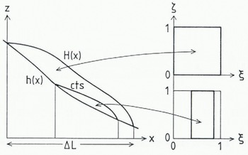
The numerical integration is performed by adopting a finite-difference scheme with centered differences in the vertical direction and upstream differences in the longitudinal direction. The method builds essentially upon the neglect of longitudinal thermal diffusion and has already been proposed by Reference Hutter, Yakowitz and SzidarovszkyHutter and others (1986). However, unlike them, we have mapped the domain (between the glacier surface and the base or the CTS, respectively) on to the unit square by the transformation (Reference PhillipsPhillips, 1957; Reference Hindmarsh and HutterHindmarsh and Hutter, 1988)

(12)

where h(x) denotes the lower and H(x) the upper boundary of the domain (Fig. 4), and ∆L is the length of the glacier. In a cross-section with only cold ice, H is to be identified with the free surface and h with the base. In a cold-temperate cross-section, two variants are possible: when H corresponds to the free surface and h to the base and to the CTS (if and where it occurs), then the cold part is looked at; alternatively, when H is identified with the CTS and h with the base, then the cold part is looked at; alternatively, when H is identified with the CTS and h with the base, then the temperate-ice region is considered. Equations (1) and (2) and the equations for the boundary conditions must be transformed accordingly; more details have been given in Reference Hindmarsh and HutterHindmarsh and Hutter (1988).

Fig. 4. Illustrating the transformation (Equation (12)) with appropriate interpretation 0/ h(x) and H(x); the cold part oF the glacier is mapped on to the unit square and the temperate part on to the rectangle.

The numerical forward integration is performed in the curvilinear coordinates, Equation (12), using the above-mentioned implicit finite-difference scheme. The conditions at the grid points at the upper or lower boundary are either a given value for temperature or moisture content, or a prescribed gradient. The conditions for moisture at the melting CTS are zero moisture content; at the freezing CTS the latter is not specified (see discussion of Equation (3)) as it is a result of the forward integration along particle paths. The boundary conditions for moisture content along the glacier bed are calculated by integrating the moisture production along the basal trajectory (Equation (3)).

This finite-difference scheme defines a system of linear equations for either the temperature or moisture content at the grid point of the new profile. The coefficient matrix is tridiagonal and therefore makes the Gauss algorithm directly applicable. This numerical procedure proved to run stably and fast, and is also applicable in a time-dependent model (Reference RitzRitz, 1989), where the same integration strategy can be used for each time step.

The model is tailored to calculate the temperature and moisture-content distribution in a glacier with a polythermal structure as depicted in Figure 1d. The glacier is cold in most parts except for a temperate basal layer in the lower part of the ablation zone. Starting with a prescribed vertical profile at the top of the glacier and proceeding down-glacier with the numerical integration of Equations (1) and (2), a typical run of the model displays the following sequence of computational steps (Fig. 5):

• (1) The first section of the glacier is wholly cold with a cold sole. The vertical temperature profiles are calculated with a given surface temperature and a prescribed vertical temperature gradient (geother-mal heat flux) at the base.

• (2) As soon as the resulting basal temperature begins to increase above the melting temperature, the basal condition is switched to a given temperature, Tm, and the basal temperature gradient is a result of the integration.

• (3) As soon as the basal temperature gradient becomes positive, an internal CTS with melting conditions is assumed. The temperature gradient at the CTS is then set to zero and the position of the CTS is calculated iteratively by shooting for the melting temperature at the CTS. Once the position of the CTS is determined on the vertical profile in question, the moisture content in the temperate part of the profile with zero moisture at the CTS is calculated. The evolving CTS is tested for the melting condition by comparing the slope of the velocity vector with the slope of the CTS.

• (4) As soon as freezing conditions are encountered, the distribution of moisture in the same profile is calculated again, this time by calculating the moisture content at the CTS via the forward integration of the advection-production Equation (3) along the flowline from point A in the melting part to point B in the freezing part of the CTS. The temperature profile is then recalculated, now by taking into consideration conditions (5), (6) and (11) for a freezing CTS. The position of the CTS in the subsequent profiles is determined by taking the moisture content at the CTS from the preceding profile and iterated by using the transition conditions (5), (6) and (11) again.

• (5) Once the CTS reaches the base, the temperature profiles are calculated again with either melting temperature or geothermal gradient at the base.

Fig. 5. The five different regimes for integrating the thermal and moisture-transport equations. The dashed line indicates the 0°C (melting-temperature) isotherm.

Treatment of the conditions at a freezing CTS turned out to be difficult and the iteration for determining the position of the CTS had to be tuned carefully to the local conditions. This problem is not yet solved to our satisfaction for all situations and warrants improvement. However, we regard a successful integration for our restricted polythermal ice sheet as a success, for it is unique and demonstrates that the model equations, that were proposed earlier by Reference HutterHutter (1982) and Reference Hutter, Blatter and FunkHutter and others (1988), are suitable in qualitatively and quantitatively describing the anticipated physical processes. A further refinement may lie in a time-dependent model which is able to handle a moving freezing CTS, but keep all other conditions stationary. Such a procedure will be a first step towards a fully time-dependent thermomechanical model.

In this work a good deal of approximation was used. Test runs showed that the position of the freezing CTS is very close to a "hybrid" CTS along which zero temperature and zero temperature gradient (as for a melting CTS) are applied. The application of such conditions is also justified for other reasons: the calculated moisture content within and along the freezing CTS strongly depends on the prescribed sliding velocity which is poorly known. For this reason, no sliding velocity is introduced in the examples which do not result in an intraglacial CTS. On the other hand, the model calculation of moisture content runs into a singularity with zero sliding velocity and, therefore, some sliding must be prescribed when an internal CTS occurs. If only the occurrence and the location of a temperate base with a temperate layer above it is of interest, then the above assumption yields accurate predictions of the location of the CTS which cannot be improved with the presently available data base. In such a calculation, the position of the CTS only depends on the conditions in the cold part of the glacier, specifically on the surface temperature, the velocity field and the ice thickness. The calculation of the moisture content remains a problem, as it depends not only on strain heating but also on basal sliding conditions, which are poorly known. The present empirical information on basal moisture content and sliding is inadequate and is not likely to be improved very much in the near future. For these reasons, no numerical results of moisture content are presented in this work.

Sensitivity Studies with Laika Glacier

Modelling Present-Day Laika Glacier

In a first run of the model, the geometry, surface temperature, horizontal surface velocity and mass-balance distribution were taken from measurements on the glacier. These boundary conditions are depicted in Figure 6. The longitudinal component of the velocity field was calculated by using the surface values, vanishing basal sliding, and an interpolation with a fourth-order parabola according to a Glen-type flow law with exponent n = 3 and a constant flow-law parameter. The vertical velocity was taken to be proportional to the distance to the glacier bed, reaching the value of the mass balance in meters ice equivalent at the surface. The physical properties of ice used in the model are given in Tabel 1. The geothermal temperature gradient was estimated to be G = 0.019Km⁻¹. Strain heating was calculated by assuming an average inclination γ = 8° of the glacier bed, as indicated in the previous section. These conditions, however, yielded a wholly cold glacier with a cold base contradicting measurements. Figure 7 displays the calculated isotherms through the glacier for this situation and indicates that the glacier is warmest at the base of the ablation zone but does not reach the melting point anywhere. The isotherms reflect a strong influence of longitudinal advection of heat. In the accumulation zone, this advection is reponsible for the conspicuous inversion in the temperature profiles; in the ablation zone, isotherms are grossly parallel to the surface and thus temperature profiles show a monotonic increase in temperature with depth.

Fig. 6. Laika Glacier: prescribed surface temperature, T_s, longitudinal surface velocity, us, and vertical surface velocity, v_s, as inferred and interpolated from surface temperature and surface mass-balance measurements. The scale on the abscissa indiates the distance to the upper end of the glacier.

Fig. 7. Laika Glacier; computed isotherms for the data shown in Figure 6 and described in the text. Notice that melting conditions are nowhere reached. The basal boundary condit-ion was no-slip throughout.

Table 1. Physical properties of pure ice as used in the numerical calculations

This increase is a result of the peculiar distribution of the near-surface temperatures. The rather high 10 m temperatures near the equilibrium-line altitude generate relatively high intraglacial temperatures which are ad-vected down-glacier. This advection, of course, is increased when an additional sliding component is introduced in this area. As a result, the calculated basal temperatures in the ablation zone correspondingly increase, but they still do not reach the melting point at the bed.

An interesting feed-back mechanism can be noticed in this result: sliding in the lower part of the glacier increases the basal temperatures due to the increased advection of the relatively warm ice in the central part of the glacier. The consequence of this fact is intriguing: once a temperate sole is formed in the ablation zone, this state is supported and stabilized by the onset of sliding. Substantiation of this effect would require solution of the coupled thermomechanical problem. We think that, with our rough estimate of the velocity field, the major inferences are unaltered. If correct, the results suggest that the observed polythermal state of Laika Glacier may be a remnant of earlier conditions, and that this state can remain stable even under climatic conditions that are not quite sufficient to produce it. This hysteresis effect should be able to be tested in a time-dependent model.

Past Laika Glacier

The above-described calculations do not reproduce the measured thermal conditions of Laika Glacier. However, Laika Glacier is rapidly retreating and the surface of its piedmont tongue is lowering at a rate of roughly 1 m year⁻¹. Thus, the glacier is certainly not in equilibrium with the present climate and the polythermal structure is suspected to be a remnant of earlier conditions, e.g. during the Little Ice Age. It is the main purpose of the following model calculations to find possible previous conditions which could explain the present polythermal structure of Laika Glacier.

Various sensitivity tests were performed by varying the geometry, mass balance, surface temperature and strain heating within a range believed to be realistic, found by measurements in various years, or reconstructed according to moraines or trim lines (Reference Blatter and KappenbergerBlatter and Kappenberger, 1988). However, the information available is sparse and the possible range of input data must be guessed by using results of other investigations concerning near-surface temperatures and mass-balance zones (Reference Hooke, Gould and BrzozowskiHooke and others, 1985; and references therein). Furthermore, the steady-state calculations cannot "prove" the hypothesis that transient effects are responsible for the present temperature distribution in Laika Glacier, but may encompass the range of conditions leading to polythermal structures.

The example which is described below assumes a variable geometry with up to 50% thicker ice than at present in the ablation zone, which is considered possible for Little Ice Age conditions according to an observed trim line at one side of the glacier. This increase in thickness of the glacier requires corresponding adjustment of other input quantities which are discussed below.

Strain Heating and Advection

The longitudinal component of the velocity was increased corresponding to the increased thickness of the ice (Fig. 8). The flow-law parameter was again assumed constant as in the first model calculations.

Fig. 8. The same as Figure 6, except for the reconstructed Little Ice Age Laika Glacier. The line labelled ub, gives the prescribed basal sliding velocity.

Ablation

A higher surface in the ablation area is likely to be more exposed to frequent strong winds on the island (Reference Blatter and KappenbergerBlatter and Kappenberger, 1988). This may have led to increased erosion of the snow cover; the winter accumulation may have been smaller and, additionally, have led to an earlier onset of ice ablation in the summer. On the other hand, the air temperatures were lower (Reference Jones, Wigley and KellyJones and others, 1982) at least during winter. This makes an estimation of the past ablation difficult. Therefore, we have used the same mass-balance distribution as for the present conditions (Fig. 8).

Near-Surface Temperatures and Advection of Heat

The surface temperature that is typical for the location of the glacier depends less on the altitude above sea level than on the Zonation of the mass balance. In the present situation, no firn accumulation occurs and consequently no percolation zone exists that could lead to higher near-surface temperatures due to latent-heat flux. Conditions may have been different during the Little Ice Age, when the annual mean temperature was substantially lower. A shift from the present superimposed ice accumulation to a percolation zone in the past may have been accompanied by a corresponding shift to higher near-surface temperatures in the highest parts of the glacier. Taking all these considerations into account and staying on the conservative side, the surface temperature was chosen as for the present except for a 1 K increase in the uppermost part of the glacier (Fig. 8).

Sliding

In this steady-state model, sliding does not affect the temperature distribution further up-glacier and therefore is not significant for the upper edge of the temperate sole along the glacier bed. Realistically, sliding with significant velocities only occurs at places with a temperate sole and must only be introduced in these places. The prescribed basal sliding is depicted in Figure 8. The values were chosen as small as possible, but large enough to prevent too high a moisture content in the basal layer.

The result of the calculation with the above-described boundary conditions and geometry is depicted in Figure 9. Except for the glacier thickness and the corresponding longitudinal ice velocity, the boundary conditions were kept close to the present-day conditions. It shows that such conservative conditions, which are considered to be realistic for the past centuries, may lead to an intraglacial CTS.

Fig. 9. The same as Figure 7, except for the reconstructed Little Ice Age Laika Glacier. The black area labelled CTS indicates the occurrence of a temperate basal layer with an intraglacial CTS.

Conclusions and Remarks on Further Work

Strain heating is the necessary mechanism to produce a near-basal intraglacial CTS. Its amount depends on the thickness of the ice and accordingly influences the basal temperatures; as can be expected, this influence is very strong. The warming tendency is responded to by the higher ice velocity in a thicker slab advecting more cold ice to lower parts of the glacier. Since the advection of the cold ice into the lower part of the glacier strongly influences the thermal conditions at the base in the ablation zone, a reconstruction of the past pattern of accumulation is essential. A relatively high firn temperature in the accumulation zone, which may have occurred in the past when the top of the glacier was in the percolation zone, leads to advection of warmer ice into the basal ice in the upper ablation zone, which thus increases the basal temperatures there.

The thermal model described above can be applied to glaciers with a polythermal structure as depicted in Figure 1d, and even more simply, to wholly cold glaciers with possibly temperate parts of the sole. Here, the model was only applied to an alpine-type valley glacier with small water content in a basal temperate layer. Our intention was to demonstrate the workability of the model equations under "realistic" conditions. It will be important to extend the range of applicability to large ice sheets where polythermal situations occur near the margin.

A closer examination of the transition conditions for zero moisture diffusivity at a melting or freezing CTS led to a simple integration procedure that enabled us to handle the two differential equations and the many boundary and transition conditions with essentially the same down-glacier marching procedure. The handling of the conditions at a freezing CTS is not yet satisfactory for all situations and warrants further refinement. A model with steady-state geometry, surface and basal boundary conditions, that allows for a time-dependent solution of the field equations and position of the CTS may solve this problem. The model could be used to calculate the steady state as an asymptotic solution emerging from an assumed initial state, e.g. the above-described steady-state solution with an approximate location of the CTS.

In this sense, our model is an important step towards the development of a fully time-dependent thermomech-anical model of polythermal ice masses. It allows for an analysis of the boundary conditions leading to a polythermal structure and permits a sensitivity study of the position of a possible CTS to these boundary conditions. However, the thermal conditions at various depths respond with different time-scales to variations at the surface and of ice thickness. Therefore, a basal temperate layer may well be a remnant of earlier conditions in a glacier whose present conditions favour an entirely cold glacier. This calls for an unsteady, transient model that is able to handle not only time-dependent surface boundary conditions but also variable ice thickness.

Future steps towards developing a fully thermo-mechanical time-dependent model for a two-dimensional (plane-flow) longitudinal section of a shallow glacier can be anticipated. The final model may be composed of three parts: (a) a time-dependent model for calculating the thermal conditions with given geometry and flow field, (b) a stationary model (time is a passive parameter) for calculating the flow field, including sliding, for a given geometry and thermal condition, and (c) a kinematic model that determines the evolution of the boundaries (ice surface and CTS) by applying the results of the other two models and the prescribed mass balance.

A time-dependent model will require setting the lower boundary deeper into the bedrock, deep enough to ensure that there are no time-dependent subglacial variations in the temperature for the period under consideration (Reference RitzRitz, 1987). Such a model will certainly extend the range of applicability; however, the requirement for data concerning the present state of the glacier and its history since the Little Ice Age will also substantially increase.