


1. INTRODUCTION
Debris-covered glaciers are common in high mountain ranges, from the Hindukush–Karakoram–Himalaya (HKH) (Scherler and others, Reference Scherler, Bookhagen and Strecker2011) to the European Alps (Brock and others, Reference Brock2010), the Caucasus (Lambrecht and others, Reference Lambrecht2011) and the Andes of Chile (Janke and others, Reference Janke, Bellisario and Ferrando2015) and can represent a considerable portion of the entire glacierized area (Scherler and others, Reference Scherler, Wulf and Gorelick2018). They have traditionally been studied less in comparison to debris-free glaciers, but are receiving increasing attention since their role in mountain areas such as the HKH region seems of importance to understand both glacier mass changes and water resources (Benn and others, Reference Benn2012; Nuimura and others, Reference Nuimura, Fujita, Yamaguchi and Sharma2012; Kraaijenbrink and others, Reference Kraaijenbrink, Bierkens, Lutz and Immerzeel2017). Studies in the Caucasus (Popovnin and Rozova, Reference Popovnin and Rozova2002; Stokes and others, Reference Stokes, Popovnin, Aleynikov, Gurney and Shahgedanova2007) and the European Alps (Deline, Reference Deline2005; Gardent and others, Reference Gardent, Rabatel, Dedieu and Deline2014) have suggested that debris extent is increasing with a warming climate and more negative glacier mass balances, while Herreid and others (Reference Herreid2015) observed a stable debris cover with a more stable mass balance in the Karakoram. Debris controls the surface ablation of the debris-covered tongues and a thin layer of debris enhances the melt rate by lowering the albedo, whereas a layer thicker than a few centimetres insulates the ice and reduces melt (Østrem, Reference Østrem1959; Mattson and others, Reference Mattson, Gardner and Young1993; Mihalcea and others, Reference Mihalcea2006; Nicholson and Benn, Reference Nicholson and Benn2006; Evatt and others, Reference Evatt2015). Recent studies have since attempted to increase our understanding of debris-covered glaciers, from the meteorology (Collier and others, Reference Collier2014; Shaw and others, Reference Shaw2015; Steiner and Pellicciotti, Reference Steiner and Pellicciotti2016; Steiner and others, Reference Steiner2018) to the actual mechanisms of mass loss and gain (Pellicciotti and others, Reference Pellicciotti2015; Ragettli and others, Reference Ragettli, Bolch and Pellicciotti2016) to the evolution and changes in the thickness and properties of debris (Shukla and others, Reference Shukla, Gupta and Arora2009; Shukla and Qadir, Reference Shukla and Qadir2016; Gibson and others, Reference Gibson2017a,Reference Gibsonb; Anderson and Anderson, Reference Anderson and Anderson2018; Woerkom and others, Reference Woerkom, Steiner, Kraaijenbrink, Miles and Immerzeel2019).
A striking feature on many debris-covered glacier tongues is supraglacial ice cliffs and ponds, features that have been observed on glacier surfaces for many decades (Müller, Reference Müller1968; Inoue and Yoshida, Reference Inoue and Yoshida1980) but have only gained scientific attention in the last two. We refer to ice cliffs as any exposed ice surface visible on an otherwise debris-covered surface. Generally these surfaces are steeper than ~30°, a critical slope below which ice accumulates debris cover (Herreid and Pellicciotti, Reference Herreid and Pellicciotti2018; Buri and Pellicciotti, Reference Buri and Pellicciotti2018). Cliffs can vary in size, exposition and geometry, ranging from relatively smooth features of only a few metres in width and height to ice walls more than 100 m in width and 30 m in height that exhibit overhanging parts as well as vertically and horizontally varying slope and exposition. A number of studies have since investigated ice cliff melt (Sakai and others, Reference Sakai, Nakawo and Fujita1998, Reference Sakai, Nakawo and Fujita2002; Han and others, Reference Han, Wang, Wei and Liu2010; Reid and Brock, Reference Reid and Brock2014; Steiner and others, Reference Steiner2015; Buri and others, Reference Buri2016a,Reference Buri, Pellicciotti, Steiner, Miles and Immerzeelb) and melt from supraglacial ponds (Sakai and others, Reference Sakai, Takeuchi, Fujita and Nakawo2000; Miles and others, Reference Miles2016) at the scale of single features and found strong indications for enhanced local ablation, however with spatial and seasonal variability. Only few recent studies have looked at the glacier scale and processes controlling where, when and how these features appear, persist and disappear, specifically in the Langtang (Kraaijenbrink and others, Reference Kraaijenbrink, Shea, Pellicciotti, De Jong and Immerzeel2016; Miles and others, Reference Miles, Willis, Arnold, Steiner and Pellicciotti2017b; Buri and Pellicciotti, Reference Buri and Pellicciotti2018) and Everest region (Thompson and others, Reference Thompson, Benn, Mertes and Luckman2016; Watson and others, Reference Watson, Quincey, Carrivick and Smith2016, Reference Watson, Quincey, Carrivick and Smith2017; Brun and others, Reference Brun2018) of the Nepalese Himalaya. Watson and others (Reference Watson, Quincey, Carrivick and Smith2017) note that ponds bordering a cliff were much larger than other ponds, that half of the observed ice cliffs bordered a pond, and ice cliffs bordering ponds were longer than others. This indicates that the two features appear in combination and their formation process is possibly linked.
Thompson and others (Reference Thompson, Benn, Mertes and Luckman2016) attributed 40% of ice mass loss to ice cliffs on Ngozumpa Glacier in recent years, while both Ragettli and others (Reference Ragettli, Bolch and Pellicciotti2016) and Watson and others (Reference Watson, Quincey, Carrivick and Smith2017) linked surface lowering rates to a higher density of cliffs and ponds in the Langtang and Khumbu region respectively. Both Miles and others (Reference Miles, Willis, Arnold, Steiner and Pellicciotti2017b) and Watson and others (Reference Watson, Quincey, Carrivick and Smith2016) found a high temporal variability of ponds, with an increase of total ponded area in the summer months and higher densities at shallower slopes and around tributaries. Kraaijenbrink and others (Reference Kraaijenbrink, Shea, Pellicciotti, De Jong and Immerzeel2016) determined 1.80 and 1.66% of Langtang Glacier to be covered by cliffs and ponds, respectively. Using high-resolution imagery from unmanned aerial vehicle (UAV) flights they however also showed that a considerable number of ponds is missed with satellite imagery of even 5 m resolution. Studies also show that most of the ice cliffs are north-facing supporting the hypotheses that ice cliffs generally survive because of shading from direct solar radiation (Sakai and others, Reference Sakai, Nakawo and Fujita1998; Kraaijenbrink and others, Reference Kraaijenbrink, Shea, Pellicciotti, De Jong and Immerzeel2016; Watson and others, Reference Watson, Quincey, Carrivick and Smith2017; Buri and Pellicciotti, Reference Buri and Pellicciotti2018). However, beyond Watson and others (Reference Watson, Quincey, Carrivick and Smith2016) and Watson and others (Reference Watson, Quincey, Carrivick and Smith2017) no studies have investigated ice cliff and pond occurrence and development on more than a single glacier and these studies lack corresponding DEMs to investigate actual area and exposition.
1.1. Aims of this study
Applying a manual delineation process, we have created a quality-controlled inventory of ice cliffs and ponds for the glaciers of the Langtang Valley, encompassing seven observation periods spanning the period 1974–2015. The availability of repeat DEMs and high-resolution orthoimages allows this study to advance previous efforts, and to document area, exposition and development of these features and to identify different types of cliffs and ponds on all glaciers in the catchment. Based on this inventory we aim to provide a better understanding of how these features vary in time and space.
Our specific objectives, beyond establishing such a dataset, are to (a) provide a first assessment of how common such features are, what percentage of the total glacier area they cover and whether this distribution changes between years and seasons; (b) determine where on the glacier ice cliffs and supraglacial ponds are most prevalent; (c) characterize the distribution of ice cliff sizes, shapes and orientations and (d) investigate how select cliff–pond systems develop from their emergence to their disappearance.
2. STUDY SITE
The upper Langtang catchment in the Nepalese Himalaya (28° 15′E, 85° 30′N, Fig. 1) extends over an area of 350 km2, ~30% of which is glacierized (Ragettli and others, Reference Ragettli2015). The five valley glaciers all have debris-covered tongues. This debris-covered area accounts for 25% of the total glacierized area and exhibits a variety of shapes, sizes, flow directions, topographic settings and surface velocities (Table 1).
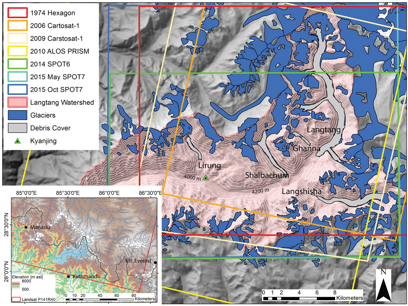
Fig. 1. Overview of Langtang catchment with the investigated glaciers, with contours derived from the SRTM DEM (Jarvis and others, Reference Jarvis, Reuter, Nelson and Guevara2008). Glacier outlines are from the RGI (Pfeffer and others, Reference Pfeffer2014), debris outlines were manually delineated and are shown for the year 2015 (Ragettli and others, Reference Ragettli, Bolch and Pellicciotti2016).
Table 1. Debris-covered glaciers investigated in this study. The values correspond to the state of the glaciers in October 2015

The maximum debris elevation refers to the highest elevation where continuous debris is encountered on the tongue.
Langtang Glacier is the longest and largest glacier in the catchment, with the debris-covered tongue longer than 15 km (Fig. 1). It has three smaller tributary glaciers. Large portions of the ablation area are directly connected to steep headwalls that regularly supply ice and debris through gravitational mass movements. Langshisha Glacier is the only glacier in the valley flowing westward (Fig. 1). Small tributary glaciers contribute mass from the lateral flanks and the glacier is flowing in a meandering way to its terminus, which is disintegrating rapidly. The accumulation area of Shalbachum Glacier detached from the ablation area at a steep section where the glacier turns towards south-east (Fig. 1). It is unique for the fact that its tongue fills nearly the entire valley in width and the moraines lead directly into steep headwalls to either side. The ablation area of Lirung Glacier is currently detached from the accumulation zone and parts of the glacier tongue are stagnant (Fig. 1). Ghanna Glacier is the smallest glacier in the catchment and shows little evidence of surface ponds in Landsat imagery (Miles and others, Reference Miles, Willis, Arnold, Steiner and Pellicciotti2017b). As with Lirung Glacier, it has very low flow velocities through the debris-covered tongue but maintains a dynamic connection through an icefall to a snow and ice source.
The catchment's weather is defined by the monsoon (mid-June to mid-September), and most of the precipitation falls during this period (Immerzeel and others, Reference Immerzeel, Petersen, Ragettli and Pellicciotti2014), while pre-monsoon (March to mid-June) and post-monsoon (mid-September to November) are dry. At higher elevations solid precipitation falls during winter from December onwards (Stigter and others, Reference Stigter2017). Because of less cloud cover the pre-monsoon season receives a higher radiation input than monsoon with relatively warm temperatures, while in post-monsoon temperatures drop quickly (Immerzeel and others, Reference Immerzeel, Petersen, Ragettli and Pellicciotti2014; Ragettli and others, Reference Ragettli2015).
3. DATA AND METHODS
3.1. Compilation of the inventory
We used high-resolution stereo satellite imagery (1.5–9 m) processed into corresponding orthoimages and DEMs from seven different seasons to identify ice cliffs and supraglacial ponds manually (Table 2; see Ragettli and others (Reference Ragettli, Bolch and Pellicciotti2016) for all details regarding the production of DEMs). We also used surface velocity data derived from 2009 and 2010 images (Ragettli and others, Reference Ragettli, Bolch and Pellicciotti2016), to assist with the interpretation of distribution patterns of cliffs and ponds. The specific dates were chosen based on image quality and availability. No images are available from the monsoon due to near-continuous cloud cover. Two of the images are from the pre-monsoon season (April 2014, May 2015), three from the post-monsoon season (October 2006, November 2009, October 2015) and two from the winter season (November 1974, December 2010). Delineations were impacted in 2010 by patchy snow cover, which possibly resulted in fewer cliffs and ponds being captured. In April 2014 a part of Langtang Glacier was not captured (Fig. 1). The images in 2015 are affected by the earthquake that took place in April 2015, as a large amount of ice, snow and debris was deposited on Langtang, Langshisha and Lirung Glacier (Ragettli and others, Reference Ragettli, Bolch and Pellicciotti2016). Due to the coarse resolution of the DEM in 1974 (30 m) no analysis of topographic parameters of individual cliffs and ponds was attempted with this dataset.
Table 2. Satellite imagery used for this study. Resolution is given for Orthophoto and DEM, respectively

See Ragettli and others (Reference Ragettli, Bolch and Pellicciotti2016) for more details on the satellite products.
3.2. Uncertainty analysis
A number of uncertainties are introduced by the variable data quality of DEMs and orthoimages. While the error introduced by missing imagery and snow or landslide cover is random and impossible to quantify, we can estimate the error introduced by manual delineation, image resolution and DEM quality. Manual feature delineation is susceptible to user errors due to poor image quality, unfavourable light situations or a wetted or snow-covered debris surface (Paul and others, Reference Paul2013; Herreid and Pellicciotti, Reference Herreid and Pellicciotti2018). To ensure an inventory as unbiased as possible, we implemented a four-step process including three different researchers viewing the data independently (Fig. 2). One person manually delineated all ice cliffs and ponds based on the orthoimages only, then a second person checked the complete inventory visually and eventual omissions and errors were corrected. A third person then used the inventory and compared it to slope maps of concurrent DEMs, as steeply sloped surfaces are a strong indicator for cliffs (Herreid and Pellicciotti, Reference Herreid and Pellicciotti2018). To maintain the independence of this interpretation, this was carried out without seeing the orthoimages. Using these data the third person identified false-positive and possible false-negative cliff outlines, again prompting an update of the complete inventory. The first person then used an algorithm described in Miles and others (Reference Miles, Willis, Arnold, Steiner and Pellicciotti2017b) using the multispectral information from near-contemporaneous Landsat imagery to identify ponded areas, a process not implemented for 1974 due to the lack of suitable scenes. This was compared to the pond inventory to add water bodies that were visually difficult to determine because of similar shade as the surrounding terrain.
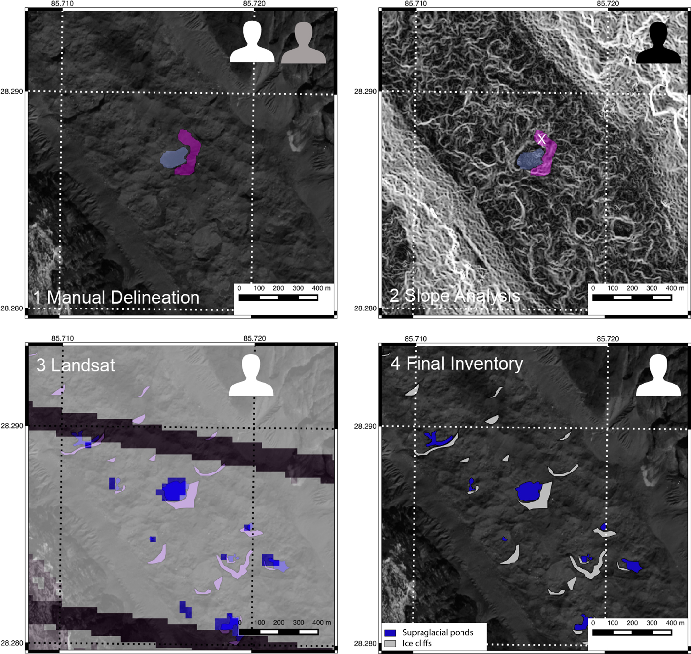
Fig. 2. Workflow to delineate ice cliffs and supraglacial ponds, involving three individual investigators. Step 1 includes manual delineation by investigator 1 and checking by investigator 2. In step 2, investigator 3 identifies potential cliffs based on the slope map without previous knowledge of the orthoimage. In step 3, Landsat images are used to classify water bodies. In step 4 the complete inventory is created based on outcomes from the initial steps.
We tested operator bias in delineation (step 1 above) by randomly selecting 36 cliffs and ponds each that were delineated by three persons independently and compared to the outlines used in this manuscript. We quantify the quality of our outlines by calculating the mean of the overlapping area between the three additional outlines and the final outline of the inventory, respectively, divided by the area of the final outline [%], as well as the coefficient of variation (standard deviation normalized by the mean [%]) of inclined area, slope and aspect for all features. We additionally tested the general quality and variability of the DEMs and the effect on the derived cliff areas by delineating 20 features that look somewhat similar to cliff faces on stable off-glacier terrain and extracting the resulting slopes and areas for all DEMs between 2006 and October 2015. This allows us to determine the general variability of the DEMs and provides us an additional measure of uncertainty for cliffs. Our total uncertainty for cliff area is calculated by summing the coefficients of variation for operator bias and DEM quality, assuming the mean for these samples to be equal.
 $${\rm CV}_{\rm tot} = \sqrt{{\rm CV}_{\rm ob}^2 + {\rm CV}_{\rm DEM}^2}$$
where CVtot is the total coefficient of variation (%) and CVob and CVDEM the coefficient of variation obtained from operator bias and DEM quality, respectively. For ponds CVtot is equal to CVob as pond areas are independent of DEM quality. We use this measure to describe the uncertainty of our estimates of cliff and pond area.
3.3. Ice cliff and pond characteristics
We characterized each cliff and pond by a number of descriptors, including the shape, size and association to cliff (for ponds) or pond (for cliffs). Field observations of cliffs at the study site have suggested several basic shapes: lateral cliffs are positioned perpendicular to the flow line, longitudinal cliffs are positioned along the flow line and circular cliffs have a partially or completely circular shape. Additionally cliffs at the glacier terminus were identified separately as these are generally larger and facing always perpendicular to the flow line. To not bias results for supraglacial cliffs in general these types were excluded from all statistics. All cliffs associated with ponds are marked separately, as are ponds with and without cliffs.
In addition to planimetric area we calculated actual surface area as well as slope and aspect of all cliffs from the DEMs. We used all pixels within each polygon and derive the slope to calculate the inclined area of the whole cliff. Weighted with the respective inclined area of each cell we then calculated a mean slope and vectorial mean of aspect value.
3.4. Spatial and seasonal distributions
We partitioned all glaciers into elevation bands of 50 m and binned ice cliffs and ponds to the respective band where more than 50% of their area was located. We additionally calculated the mean longitudinal gradient following Miles and others (Reference Miles, Willis, Arnold, Steiner and Pellicciotti2017b) for each bin. We performed this analysis only for the three largest glaciers in the catchment (Langtang, Langshisha, Shalbachum) as on Lirung and Ghanna the total numbers of features are very small in each individual year and at each elevation band. To not bias the analysis towards elevation bands that include tributary glaciers (on Langtang Glacier), we only investigated the statistics of the main glacier trunk for this purpose.
To investigate the persistence of cliffs and ponds we tracked all features on the largest glacier, Langtang, across images from October 2006 to October 2015. For this we checked how many of the features present in 2006 were still visible in 2009, how many of those subsequently in 2010 and so on. We judged this based on the shape and orientation of the feature respective to the glacier flow direction. We then repeated this for all features present in other years and their eventual development in future time steps. Since only part of the glacier in 2014 was covered by our imagery, we did not compare earlier data to this time step, but only how many of the features present in 2014 were still present in 2015. Since the time period between 1974 and 2006 was too large to determine whether a feature in both images was actually the same, we did not investigate the earliest image available.
4. RESULTS
4.1. Uncertainty
The data used in this study are of variable quality, which impacted our ability to detect features (for optical data) as well as quantify their area (for DEMs). In 2010 parts of the glacier surfaces were covered in snow, while in 2014 a part of Langtang Glacier was not captured in our imagery and the lower part of Langtang Glacier was furthermore covered by deposits of a co-seismic landslide in May 2015. These artefacts lead to a reduced ability to detect features in these years and our total numbers of detected features is hence a lower bound estimate. Below we outline additional quantifiable uncertainties that can be attributed to our choice of data and methods, namely the uncertainty of our estimates introduced by our manual delineation, the differing resolution of stereo imagery and the quality of the DEMs.
4.1.1. Delineation quality
Comparison of delineations of randomly chosen cliffs and ponds shows that for individual cliffs disagreement on what constitutes the cliff area is most common at the outer fringes where it is difficult to ascertain whether a grey cover constitutes a darkened cliff face or actual debris cover (Herreid and Pellicciotti, Reference Herreid and Pellicciotti2018). However, the overall overlap between the outlines had a mean of 76% for cliffs and 80% for ponds. The coefficient of variation for area is 25% for cliffs and 21% for ponds. While even higher resolution data (i.e. from UAVs; Kraaijenbrink and others, Reference Kraaijenbrink, Shea, Pellicciotti, De Jong and Immerzeel2016) will potentially increase the accuracy in delineation of single features and provide a better representation of local topography, necessary for targeted modelling studies (Buri and others, Reference Buri, Pellicciotti, Steiner, Miles and Immerzeel2016b), a comparison between the image used in Kraaijenbrink and others (Reference Kraaijenbrink, Shea, Pellicciotti, De Jong and Immerzeel2016) and the overlapping area of the SPOT image from April 2014 shows no significant area difference in the delineation of visible cliffs and ponds. These results show that while manual delineation of optical satellite imagery is suitable to derive an estimate of cliff and pond areas on the glacier scale, errors may nonetheless be considerable for individual features. We have hence made sure to exclude features or parts of features that can not be absolutely asserted to be a cliff or pond in the four-step process outlined above, which was especially the case for images with snow cover (2010) and poor illumination (2014). As a consequence the results we present are a minimal estimate in respect to the total area of cliffs and ponds. The mean coefficient of variation of slope and aspect are just 6% (1.9°) and 7% (13.3°), respectively, suggesting that an error in delineation does not have strong impact on the interpretation of these topographic variables.
4.1.2. Stereo image quality
We compared all pixels identified as an ice cliff and found that the median slope in the DEMs with 3 m resolution (2014–2015) is with 28.3° slightly higher than for the coarser DEMs with 5 m resolution (2006–2010, 28.2°) and while 9% of the pixels are steeper than 50° for the higher resolution data, only 7% for the coarser data are. As a result, the cliff area in the earlier years may be underestimated if we assume that cliffs did not actually steepen over time. To test this possible bias, we selected 20 features on stable off-glacier terrain that resembled cliffs visually. The mean area of these features was 5470 m2 in the 5 m data and 5680 m2 in the 3 m data, corresponding to an increase of 4%, with a coefficient of variation of 8% between all years. Due to the high resolution of our satellite data, our lower threshold of optical detection is 3–5 m2 and we argue that exposed ice or water below that area is likely so ephemeral, that they are of little interest to potential mass loss of ice. DEM resolution is coarser (9–25 m2), but only 1 cliff and 2 ponds in our whole inventory are smaller than 25 m2 and only 35 features are smaller than 50 m2. Comparing our inventory in the lowest part of the Langtang tongue in April 2014 to the mapped features a month later using UAV imagery in Kraaijenbrink and others (Reference Kraaijenbrink, Shea, Pellicciotti, De Jong and Immerzeel2016) shows that we were able to capture all cliffs, while missing a number of small ponds, some of which may have formed in the onset of the melt period between April (SPOT overpass) and May (UAV flight). Possibly this bias increases in wet seasons, when many small water bodies appear on the surface of the debris, but more overlapping data are necessary to investigate this in more detail. Considering these uncertainties we derive a total area uncertainty of 26% for cliffs (as a result from operator bias and stereo image quality) and 21% for ponds (from operator bias alone), noting that many small water bodies are likely to be missed due to insufficient resolution of the orthoimages.
4.2. The inventory
Over all seven orthoimage/DEM sets we identified 2267 cliffs and 1039 ponds (Fig. 3 and Table 3). On the largest Langtang Glacier there are more than 150 cliffs and ~100 ponds on average. This results in ~4–24 cliffs and 3–5 ponds per km2 of debris cover on Langtang Glacier alone.
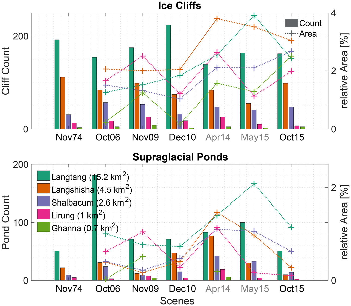
Fig. 3. Distribution of ice cliffs (top) and supraglacial ponds (bottom) over all years. Bars show numbers and crosses actual relative area covered by cliffs and ponds on the debris-covered tongue. Area values for the glaciers in the legend correspond to the debris-covered area. Months marked in grey are part of the wet, those in black are part of the dry season.
Table 3. Total cliff and pond areas over all glaciers from 2006 to 2015

All values in m2. Values in brackets are relative area of the debris-covered tongue [%]. All values are subject to a 26 and 21% uncertainty for cliffs and ponds respectively.
The total area covered by cliffs on Langtang ranged between ~ 190 000 m2 (± 49 000 m2) and 600 000 m2 (± 154 000 m2), always accounting for more than 50% of the cliff area in the catchment (Table 3). On all glaciers the total cliff area was greater in the wet seasons and in some cases more than doubled in area compared to the dry season (Table 3). Areas of ponds are overall smaller (between ~ 110 000 m2 (± 23 000 m2) and 320 000 m2 (± 67 000 m2) on Langtang Glacier) but here the inter-seasonal changes are even more extreme. Total pond area is between 1/3 and 1/2 of the total cliff area (Table 3).
While a potential systematic bias due to the use of different sensors exists, using the DEMs enabled us to account for the actual area of the cliff face which, due to the steep slope of the cliffs, is 20–25% larger than the planform area as seen on an orthoimage. This actual area is effective for melt and needed for physically based melt models. Our data cannot account for overhangs, a common feature on many cliffs (Steiner and others, Reference Steiner2015; Kraaijenbrink and others, Reference Kraaijenbrink, Shea, Pellicciotti, De Jong and Immerzeel2016).
The actual ice cliff area on individual glaciers corresponds to between 0.2% (±0.1%) and 3.0% (±0.8%) of the total debris cover in the dry seasons, with lowest values in winter, and 1.1% (±0.3%) and 3.8% (±1.0%) in the wet season. Considering the fact that we have followed a conservative approach in delineation, the real values are likely slightly larger. This seasonal difference is however not reflected in the number of cliffs, which changes but without a pattern linked to seasons (Table 3). This suggests that it is the average size of cliffs that increases in the melt season. Ponded area accounts for less than 1.1% (±0.2%) of the debris-covered area in all dry seasons and increases up to 2.1% (±0.4%) during the wetter seasons when ponds fill (Miles and others, Reference Miles2016, Reference Miles, Willis, Arnold, Steiner and Pellicciotti2017b). Contrary to ice cliffs it is the number of ponds that increases in the wetter seasons suggesting new formations with increased melting activity (Table 3).
4.3. Characteristics of ice cliffs and ponds
The median cliff area of all features is 845 m2. The largest cliffs are found on Langtang (982 m2) and the smallest on Shalbachum (566 m2, Fig. 4). Median pond area is 475 m2, with 633 m2 for Langtang and 166 m2 for Ghanna the maximum and minimum values. The smallest detected cliffs and ponds were 15 and 19 m2 respectively, the largest 25150 and 32760 m2. Separate data for all years suggest that individual cliff and pond areas increase over time on the largest glaciers and remain highly variable between years everywhere else (Fig. 4).
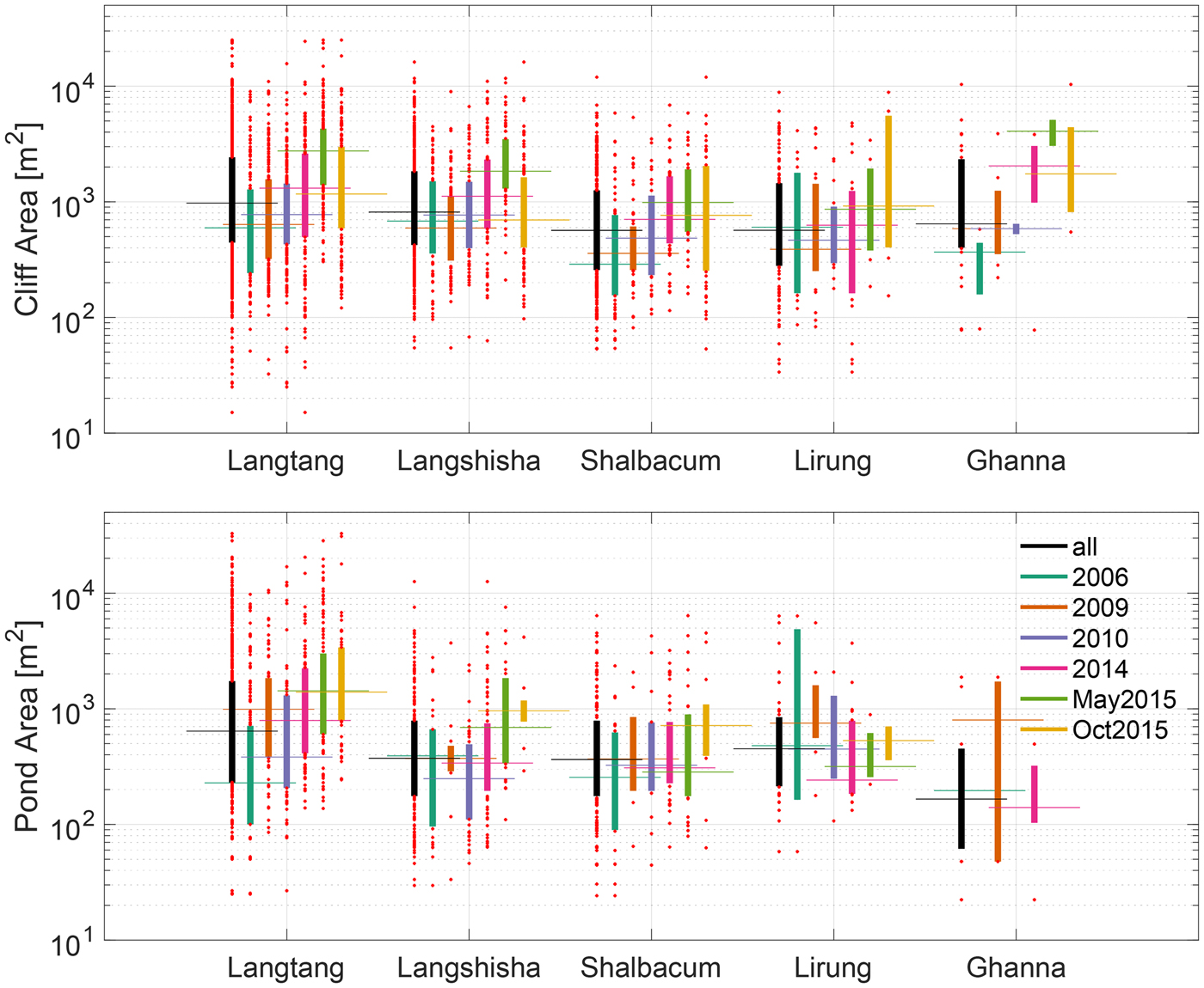
Fig. 4. Median cliff (top) and pond (bottom) areas with glaciers sorted by decreasing size from left to right, with individual scenes in different colors. The black box plot includes all years. Boxes show the 25–75th percentile, red dots are outliers.
Individual cliff areas are greatest on the largest glacier, Langtang, which also has the shallowest tongue, and are smaller on Langshisha and Shalbachum, in line with area decrease and slope increase (Fig. 4). The same holds for ponds.
No clear trends are apparent in the areas of individual cliffs and ponds for Lirung and Ghanna Glacier. Surface velocities on these two glaciers are considerably lower than on the other glaciers (0.2 and 2.7 m a−1 on average for all elevation bands in the years 2009 and 2010 compared to 6.3, 4.6 and 4.3 m a−1 for Langtang, Langshisha and Shalbachum in the same period) and relatively small numbers of cliffs and ponds point to these glaciers being dynamically much less active than their larger counterparts. A number of cliffs on these two glaciers are of the type that remain at nearly the same location with similar surface area and shape over years. Contrary to these permanent cliffs, most features identified in the inventory are of transient nature when considering a time span of multiple years (Table 5).
Although cliff orientation varies slightly between glaciers, the dominant aspect in the catchment is towards the northwest, facing away from the main direction of incoming solar radiation (Fig. 5). Fifty-three per cent of all cliffs on Langtang faced northwest (270–360°) and only 9% southeast (90–180°), on Langshisha 60% northwest, 6% southeast and on Shalbachum 39% northwest, 10% southeast (Fig. 5).
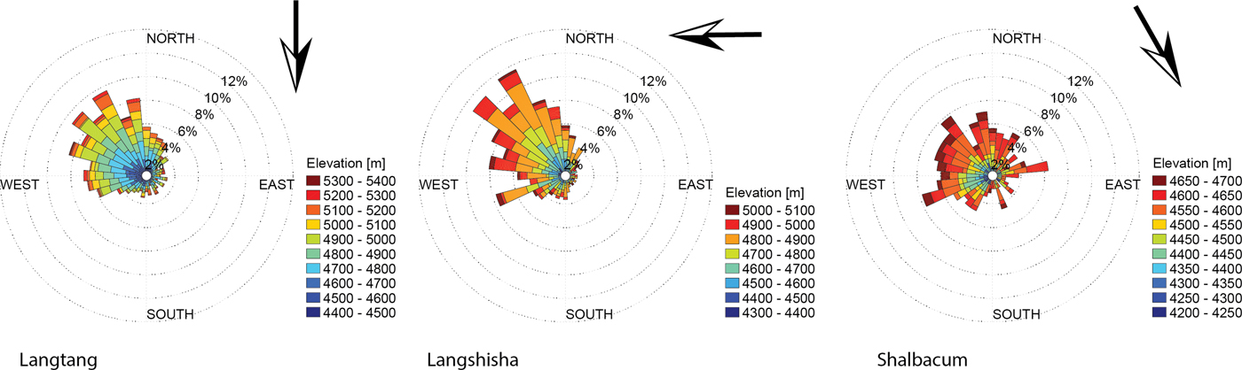
Fig. 5. Cliff aspect distribution on the three largest glaciers in the catchment. The percentages show occurrence relative to the total number of cliffs. The arrows show the principal flow direction of the glacier.
Median slope values on all glaciers are fairly consistent with 26.0° (σ = 9.1°, Shalbachum), 28.4° (σ = 9.2°, Langtang) and 29.5° (σ = 9.9°, Langshisha).
4.4. Cliff and pond types and their association
Between 73 and 80% of the ice cliffs are lateral cliffs, only 10–14% are circular and the rest are longitudinal. Some cliffs never have melt water next to them (~40%), others are bordering a water body all the time but are variable in shape (~10–20%, Table 4).
Table 4. Cliffs with ponds and ponds with cliffs

Values in brackets are [%]. Ghanna is not shown as too few features exist for reasonable statistics. Seasons marked in grey are wet, seasons in black are dry.
Ponds on the other hand can occur on the surface of debris without any exposed ice close by (29% of all ponds in the catchment in all years), in the centre of a circular cliff (24%) or at the bottom of a straight lateral (41%) or longitudinal cliff (6%). Generally more than 50% of the ponds are associated with a cliff. However fewest ponds are next to a cliff consistently over all glaciers in April 2014, when melt is strongest and new ponds appear on the debris surface. In the dry seasons this value is generally above 70%. Ponds without a cliff often show low turbidity and are generally circular. Conversely, only in the wet seasons more than 50% of cliffs are associated to a pond, while in the dry seasons less than 30% are (Table 4).
Data from individual glaciers suggest that a cliff is much more likely to be associated to a pond in a dry season on the larger and more active Langtang Glacier (27%), than on the less active smaller glaciers (17%, Table 4). This difference is not apparent in the wet seasons (55% on Langtang and 55% on all other glaciers). Whether ponds are associated to a cliff or not is however unrelated to the size of the glacier.
On the three largest glaciers, cliffs associated with ponds are 12–33% larger than those without, while on Lirung this is reversed and cliffs without ponds are 25% larger. This is likely due to large stationary cliffs on this glacier where all the water has disappeared in the dry season. Cliffs that have ponds at their base are expected to be steeper due to oversteepening at the base caused by the increased melt due to the interaction with water (Miles and others, Reference Miles2016). This is not shown by our data, as we observed no clear difference in slope between cliffs with or without ponds.
4.5. Cliffs and ponds in space and time
Ice cliffs and ponds appear across the whole elevation range of debris cover in the catchment but it is obvious in all years that some areas show higher densities than others (Fig. 7).
There is a general similarity in cliff and pond distribution along the glacier tongue. While the lower part, with thickest debris, has few features, numbers and relative coverage increase up-glacier and decrease again towards the debris-emergence area where debris cover is thinnest. On Langtang this peak is at ~5.5 km from the terminus, while Langshisha Glacier has a bimodal peak and on Shalbachum the feature density only peaks just before the head of the debris cover when the glacier turns into an ice fall (Fig. 7). Areas of higher feature density also coincide with the location of the largest features on the glacier (shown for Langtang Glacier in Fig. 9). Our data also show that both cliff and pond area increase across nearly all elevation bands between the dry and the wet season (Fig. 7).
In Table 5 we present the number of cliffs and ponds that have remained through multiple images in our inventory. Of the cliffs present in 2006, only 17% were still present in October 2015, resulting in an annual disappearance of 9–13% of cliffs. The rate of disappearance appears to decrease over the years as in the early years smaller cliffs vanish more rapidly. Values are similar for cliffs present in 2009 and 2010, while the rate of disappearance is much larger from the image in 2014 and May 2015 onwards, as many of the ephemeral cliffs that appear due to local melt disappear after only one season. For ponds the initial decrease is more rapid, as many ponds completely vanish after only one season having drained, while more cliffs change their size but do not disappear completely. The eventual annual loss is similar however at ~10% a−1.
Table 5. Delineated cliffs (top) and ponds (bottom) on Langtang Glacier that persisted through the years, i.e. where present in all images between the year given in the row and the year from the column

Values are actual number of features, with percentage of initial starting value in brackets.
4.6. Cliff–pond systems
Our dataset suggests that cliffs and ponds are features appearing in combination or forming in response to the same controls, and are likely developing under similar geomorphological and ice-dynamical circumstances. We show that the number of cliffs associated with ponds varies strongly between seasons, reaching a maximum of 58–69% in April 2014 and with values below 10% in the dry seasons (Table 4). The statistics from Table 4 and Figure 9 provide some insight into the development of cliff–pond systems in time and space. Cliffs associated to ponds are often clustered together pointing to areas with high hydraulic activity and they appear most numerous in the wet seasons. These are also the seasons when more ponds without cliffs associated appear as more melt water accumulates on the surface.
The question remains how these cliff–pond systems develop over time, from their inception to their disappearance. As discussed above a number of cliff and pond types exist and these systems can both appear for only one season or remain over multiple years. We chose three common examples to visualize the evolution of such morphologies (Fig. 8).
Figure 8a shows the development of a lateral cliff-pond system (shown in Fig. 6c), which is the most common form found in this study. A pond associated to a cliff existed as far back as 2006 and has since backwasted ~100 m until October 2015. Deducting mean annual surface velocity in this location (~ 3 m a−1) this results in horizontal backwasting of ~4–5 cm d−1, assuming that melt only takes place from April to October, which seems justified based on observations from the field (Steiner and others, Reference Steiner2015). These numbers correspond closely to backwasting rates found in the catchment (Steiner and others, Reference Steiner2015; Brun and others, Reference Brun2016) and on other glaciers (Watson and others, Reference Watson, Quincey, Carrivick and Smith2017). Most of the water disappeared by December 2010 and in May 2015 the area was still covered in snow from the co-seismic avalanches and it was not possible to determine whether the pond had drained (Ragettli and others, Reference Ragettli, Bolch and Pellicciotti2016). The shape of the cliff had changed from slightly concave to straight with two convex sections. Many processes are potentially at play that may have contributed to this reorientation including calving, heterogeneous subaqueous melt and changing direction of longwave radiation from the surrounding debris as well as subsequent reburying of parts of the cliff by trundling debris. While this cliff system existed probably much earlier than 2006 and still exists in 2018 based on recent field visits, other cliffs and ponds around have appeared and disappeared within the study period. Possibly the cliff is incised deep enough to remain connected to up-glacier drainage pathways supplying more melt water, while other systems may be more superficial. The figure also shows an example of how smaller systems (e.g. the small cliff to the west in 2009 and 2010) eventually merge into another cliff significantly expanding its total area.
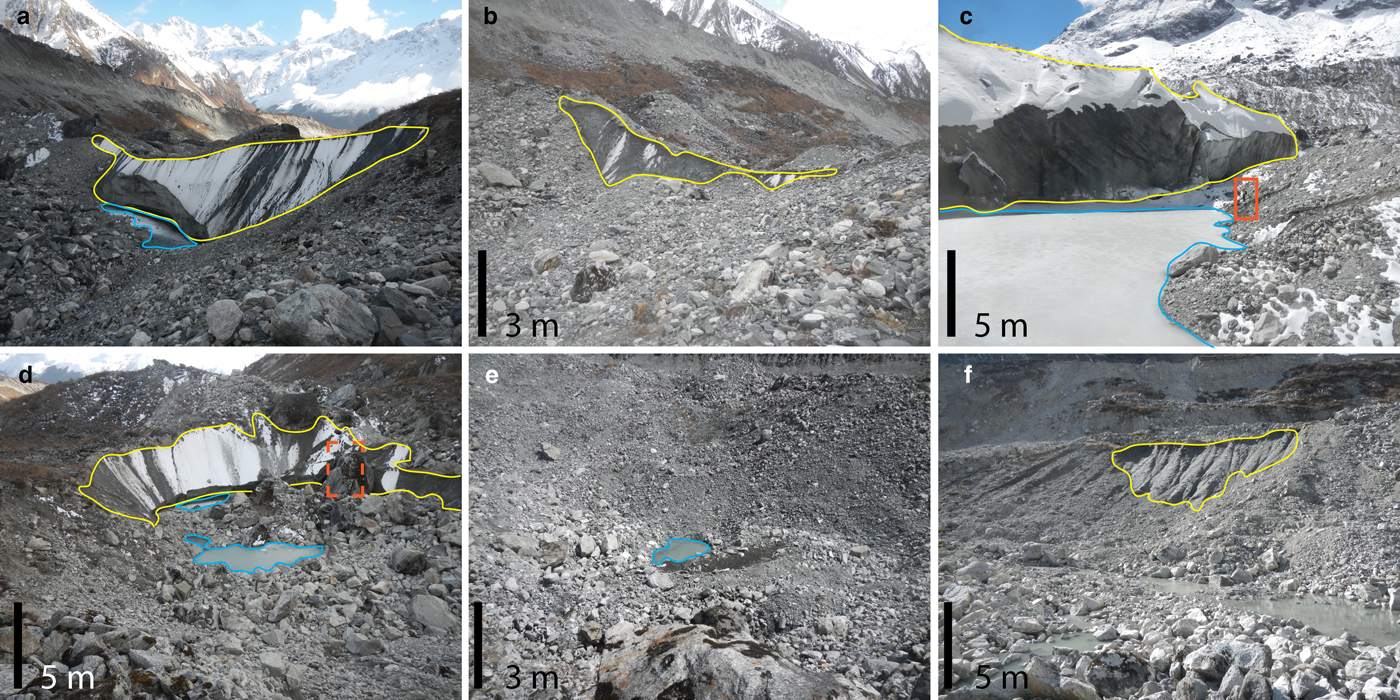
Fig. 6. Some of the main types of cliffs (yellow outline) and ponds (blue outline) found on debris-covered glaciers. (a) A medium (~120 m width) lateral cliff with a small pond. (b) A small (~10 m width) cliff about to disappear, not connected to a pond. (c) Part of a large lateral cliff (~280 m width) partially associated to a pond. A person is marked for size reference. (d) A circular (~50 m width) cliff with a pond at the centre 2 years after its initial formation. The dashed line marks an entrance to a main englacial conduit of the glacier. (e) Surface pond (~2 m width), generally not visible on satellite imagery. (f) South-facing terminal cliffs, with melt water channels engraved in the ice. All features shown were located on Lirung Glacier.
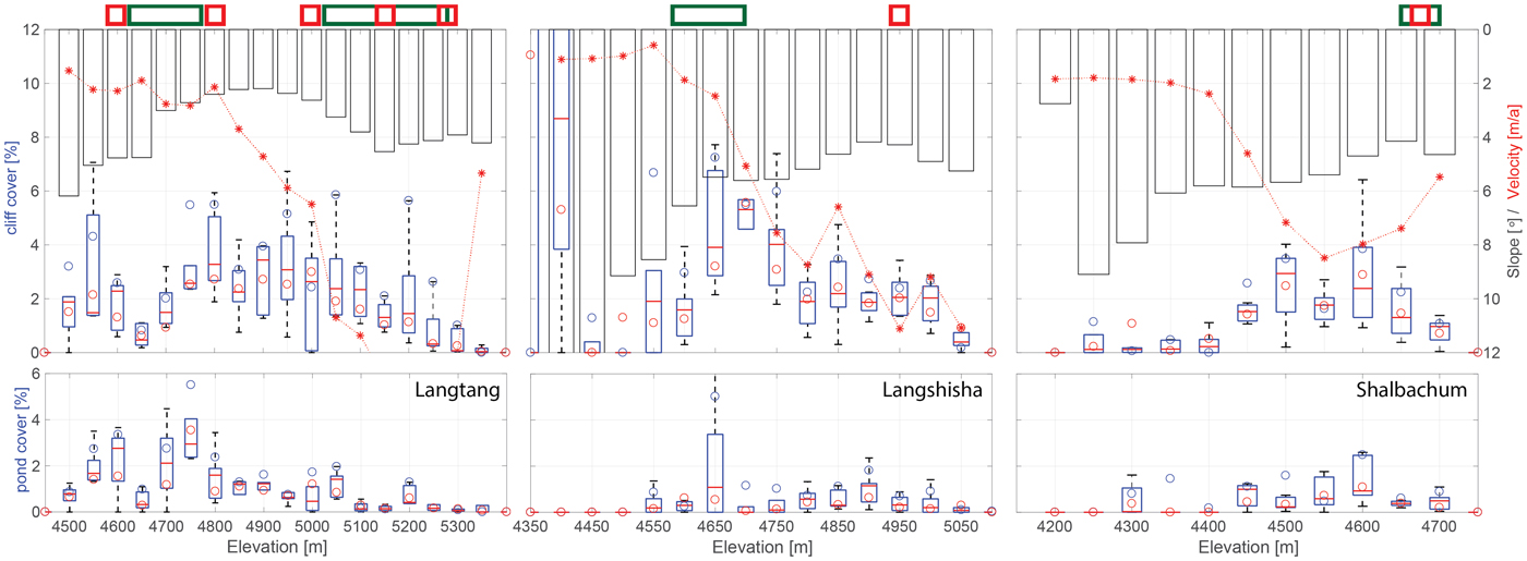
Fig. 7. Individual cliff (top) and pond (bottom) area relative to the area of the elevation band over all seasons. The blue and red circles are mean values for the wet and dry seasons respectively. Black bars and red stars in the top panel show slope and mean velocity respectively. Green squares at the top of the Figure denote areas with strong bends in the tongue, red boxes denote tributary glaciers reaching the main tongue.
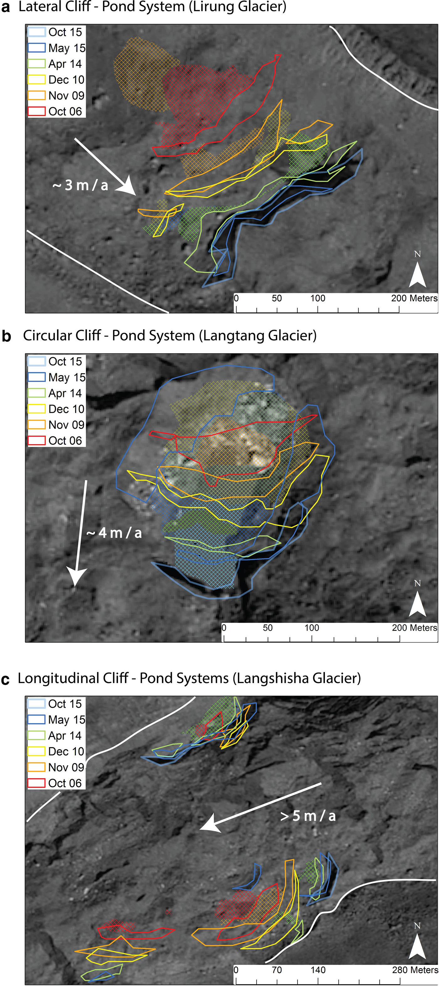
Fig. 8. Outlines of selected cliff (solid lines) and pond (cross-hatched areas) systems from October 2006 to October 2015. (a) A typical lateral cliff-pond system spanning nearly the whole tongue on Lirung Glacier. (b) A typical circular cliff-pond system between the first and second tributary on Langtang Glacier. (c) Cliffs on the side of Langshisha Glacier, bordering the moraines. Solid lines are cliffs, cross-hatched areas are ponds. White lines show the border of the glacier surface, surface velocities shown are mean velocities derived from surface displacement. The orthoimage shown is from October 2015.
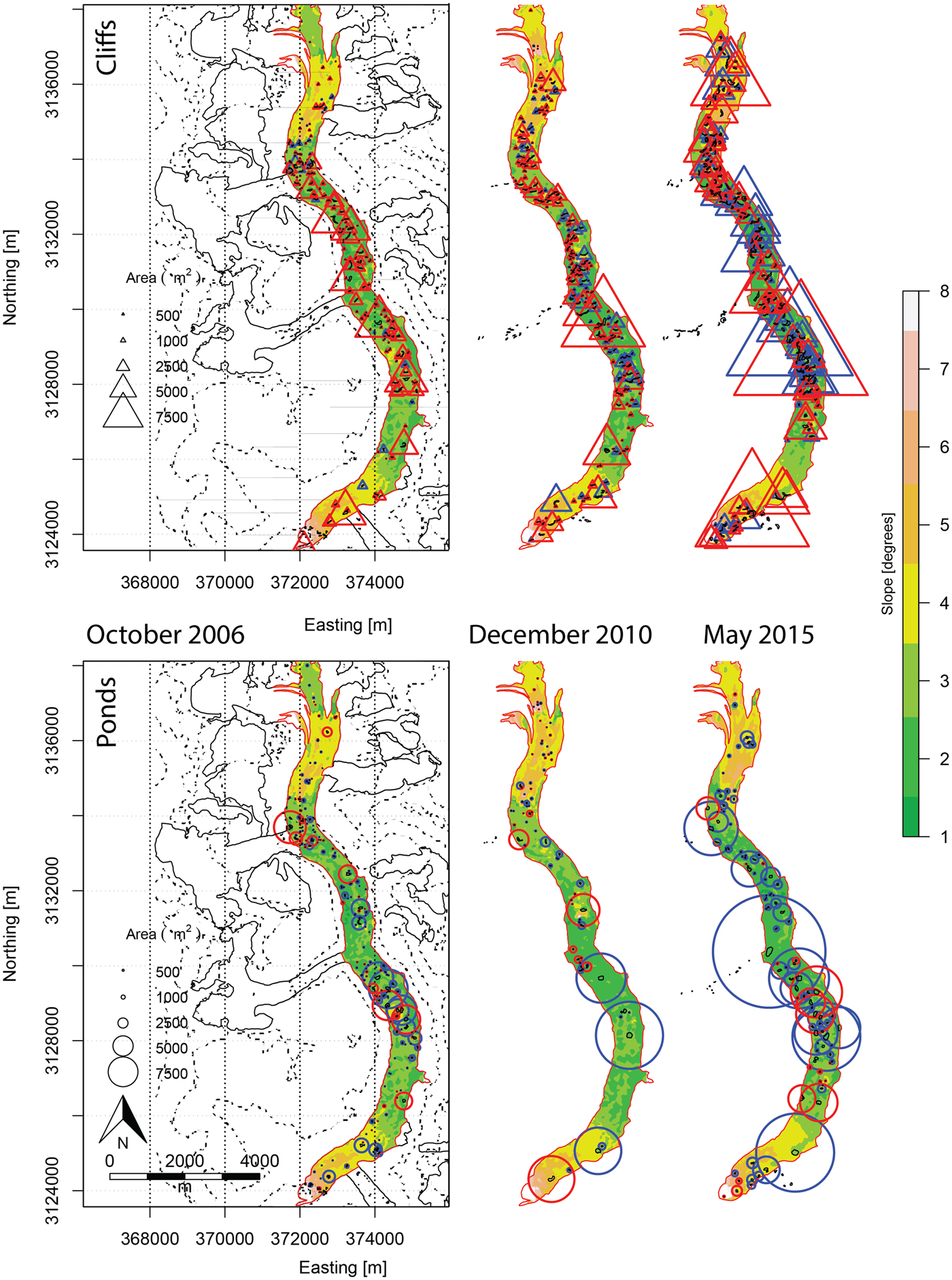
Fig. 9. Supraglacial Cliffs (top) and Ponds (bottom) on Langtang Glacier in October 2016 (dry post-monsoon season), December 2010 (winter) and May 2015 (wet pre-monsoon season). Blue markers are cliffs associated with ponds or vice versa, red are cliffs with no ponds or vice versa. The black outline is the glacier area, the red outline shows the debris cover disregarding lateral glaciers joining the main branch.
Figure 8b shows the second most common system, largely circular. A similar example is shown in Figure 6d. Initially a straight ice cliff formed which over a period of 10 years developed nearly into a full circle with a pond inside. We expect that backwasting rates are higher due to the near-continuous contact with a pond. The backwasting has been continuously accelerating since a small pond is present in 2009, which increased in size to 2010 and has since expanded southward. While the lateral cliff has moved down glacier, the northernmost part of the circular system is actually further up-glacier in 2015 than where the initial cliff formed in 2006. This system is located in the shallowest part of Langtang Glacier, which also experiences the highest rates of thinning (Ragettli and others, Reference Ragettli, Bolch and Pellicciotti2016). Here ponds are highly persistent (Miles and others, Reference Miles, Willis, Arnold, Steiner and Pellicciotti2017b) and it is possible that such a system can also sustain itself after it has intersected the hydrological base level of the glacier (Benn and others, Reference Benn2012), indicating the future development of a permanent supraglacial lake. An alternative way such circular systems can develop is the occurrence of a meltwater pond on the debris surface (Fig. 6e), that continuously downwastes and finally exposes ice walls.
Figure 8c shows the least common type, longitudinal cliffs. They are more common on Langshisha Glacier which flows from east to west, and as a result cliffs that are parallel the flow direction are most efficiently shaded. They also appear more frequently on the upper reaches of the tongue and are in general less connected to ponds and are subject to frequent change. This could be explained by the backwasting process happening perpendicular to the flow line. If the cliff was initially formed by conduit collapse but eventually receded from the location of the actual conduit by backwasting, it will eventually disappear. Additionally these cliffs could be indications of supraglacial streams which are evident on the upper reaches of Langtang and Langshisha Glacier where debris cover is thin.
All three systems shown in Figure 8 belong to the 17% of cliffs and 7% of ponds that remain on the surface over nearly a decade (Table 5). While it is obviously often such large systems that prevail, it is difficult to link persistence to characteristics like exposition, area or association to cliff or pond respectively. This is because such cliff-pond systems change their appearance over time. Ponds can be particularly variable, fluctuating between several 1000 and 100 m2 in adjacent images. While there is further potential to explore the development of individual systems in the dataset and their link to topographic characteristics, this goes beyond the scope of this study.
5. DISCUSSION
5.1. Cliffs and ponds on the catchment scale
Ice cliffs in the Langtang catchment cover an area of up to 823 000 m2 (± 214 000 m2) in the wet season, covering ~3.4% (±0.9%) of the total debris-covered area and less than half of that in the dry season (1.4% (±0.4%), Table 3). This is similar to a study focusing on Langtang Glacier alone (1.8%; Kraaijenbrink and others, Reference Kraaijenbrink, Shea, Pellicciotti, De Jong and Immerzeel2016), but considerably less than on Changri Nup Glacier in the Khumbu catchment (7–8%; Brun and others, Reference Brun2018). Using observed melt rates from the pre-monsoon season (Steiner and others, Reference Steiner2015, ~ 5 cm d−1), this results in 0.4–0.6 m3 s−1 (± 0.1 m3 s−1) runoff equivalent, which corresponds to 8–13% of the total runoff in the upper catchment in May (Ragettli and others, Reference Ragettli2015, ~ 5 m3 s−1).
For this calculation, it is essential to consider the inclination of the cliffs to assess the effective area for melt, as using the mapview area would cause an underestimation of up to 25%. Since mean slopes are similar on all glaciers, with values that we believe to be typical for an ice cliff (26–29.5°), catchment-wide estimates of real cliff area in the absence of adequate DEMs could be obtained with a factor accounting for this mean slope. More studies comparing high-resolution DEMs with less accurate satellite-derived products would however be helpful to ascertain the applicability of such a relation in other study areas.
Ponds cover less than half of the area of cliffs, as low as 0.6% (±0.1%) in the dry and 1.6% (±0.3%) in the wet seasons. Significant ponded area is missed even by high-resolution sensors as used in this study (Kraaijenbrink and others, Reference Kraaijenbrink, Shea, Pellicciotti, De Jong and Immerzeel2016) and this fraction is hence likely higher. Additionally melt from ponds is possibly higher as the water–debris/ice interface is an efficient route for the transfer of energy to the interior of the glacier (Miles and others, Reference Miles2016).
5.2. Characteristics of individual cliffs and ponds
No comparable area measurements exist for ice cliffs. Median area values for ponds (475 m2) found in this study lie between the mean values found by Kraaijenbrink and others (Reference Kraaijenbrink, Shea, Pellicciotti, De Jong and Immerzeel2016) for a small portion of the study area with higher resolution data (UAV; 252 m2) and coarser data (RapidEye; 1137 m2). They correspond well with the median for ponds in the Everest region (498 m2; Watson and others, Reference Watson, Quincey, Carrivick and Smith2016) but are well below the pond areas for a part of Ngozumpa Glacier found to be between 1500 and 2000 m2 by Thompson and others (Reference Thompson, Benn, Mertes and Luckman2016). This is likely because Thompson and others (Reference Thompson, Benn, Mertes and Luckman2016) focused on the lower, near-stagnant sections of the tongue, where larger ponds and cliffs also form on Langtang Glacier: below 4850 m the median pond size is 1180 m2. Our results suggest that ponds tend to be larger on larger glaciers, which could be due to the greater space or increase in hydrological complexity. Total pond and cliff areas tend to increase in the wet seasons (Fig. 3 and Table 3). This intuitively makes sense as lakes fill with melt water and ice cliffs grow with increasing incoming solar radiation. This is an important observation as obviously the timing of the chosen satellite imagery can have significant consequences for the final area estimates. While there is a large seasonal change for cliffs and ponds, our dataset does not indicate any significant trend in terms of total number of cliffs and ponds or its area relative to the total debris-covered glacier surface, a finding congruent with an earlier study on ponds (Miles and others, Reference Miles, Willis, Arnold, Steiner and Pellicciotti2017b). While the number of features has remained relatively stable over the years, the increase in median area points towards a coalescing of features to form larger cliffs and ponds or single cliffs and ponds ever increasing in size, which for Langtang Glacier appears to be occurring especially in a zone of low surface gradient in the centre of the tongue (Fig. 4).
The increase in individual cliff and pond areas over time suggests reduced drainage efficiency leading to a local increase of ponds and subsequently cliffs. For the upper part this could also be due to a recurring cycle of cut-and-closure of existing channels (Benn and others, Reference Benn2017). This happens as a result of increased downwasting of the ice, resulting in an increasingly hummocky surface and redistribution of debris locally. While ice cliffs and ponds are a driver of increased downwasting (Ragettli and others, Reference Ragettli, Bolch and Pellicciotti2016), this in turn may cause the formation of more and larger cliffs and ponds, resulting in an amplifying effect accelerating the demise of these glacier tongues. Locally the disintegration of englacial channels results in an increasingly heterogeneous surface with consequences for the local atmospheric convection (Miles and others, Reference Miles, Steiner and Brun2017a) and possibly an explanation for very heterogeneous debris thickness patterns observed on these glaciers.
Ice cliffs in the catchment are predominately north-facing (Fig. 5), supporting hypotheses from earlier studies (Sakai and others, Reference Sakai, Nakawo and Fujita1998; Steiner and others, Reference Steiner2015) and new recent findings (Buri and Pellicciotti, Reference Buri and Pellicciotti2018). Langshisha Glacier, flowing east to west is a case in point. Here many cliffs are of the longitudinal type, aligning with the flow rather than perpendicular to the flow, as a result of more efficient shading. The two glaciers with higher numbers of south-facing cliffs are flowing towards the south. While here melt rates are expected to be considerably higher than on other cliffs (Buri and Pellicciotti, Reference Buri and Pellicciotti2018), these cliffs will likely disappear at a slower rate because it is continuously supplied with ice flowing south. This predominately north-facing exposition – between 39 and 60% of the cliffs on individual glaciers faced north-west, while only 6–20% faced south-east – corresponds to observations by Kraaijenbrink and others (Reference Kraaijenbrink, Shea, Pellicciotti, De Jong and Immerzeel2016) for Langtang Glacier. In the Khumbu catchment Thompson and others (Reference Thompson, Benn, Mertes and Luckman2016) found that 45% of the cliffs were north-facing, 11% south-facing and 21 and 24% east- and west-facing and Watson and others (Reference Watson, Quincey, Carrivick and Smith2017) for the same region but a larger dataset found predominately north-facing cliffs.
Values obtained for slope are much smaller than what Kraaijenbrink and others (Reference Kraaijenbrink, Shea, Pellicciotti, De Jong and Immerzeel2016) obtained (30–40°) with higher resolution data. Although DEMs of the resolution used in this study (3–5 m) capture cliff features in general, they fail to accurately map the steep parts of cliffs that are much narrower than the resolution in a planform view and hence result in shallower slopes. The central portions of cliffs are generally steeper (Steiner and others, Reference Steiner2015, 35–90°). Within a 3 and 5 m pixel the elevation difference of a 50° cliff is 4 and 6.5 m respectively, causing the measured slope to be just 34 and 33°. Herreid and Pellicciotti (Reference Herreid and Pellicciotti2018) found a slope threshold value to identify cliffs on Ngozumpa as ~ 30°, which corresponds more closely to values found in this study.
For the Ngozumpa Glacier Thompson and others (Reference Thompson, Benn, Mertes and Luckman2016) found that 75.3% of the ice cliffs bordered a supraglacial pond, in an image acquired in wet monsoon (June 2010). Our data suggests a maximum value of 58–69% in the wet season and values even below 10% in the dry seasons, suggesting that a momentary observation can not be taken as the average value, and most of the year the association may be low as surface water fluctuates (Miles and others, Reference Miles2016). Similarly Watson and others (Reference Watson, Quincey, Carrivick and Smith2017) show that 30–76% of ice cliffs have an adjacent pond, with an average of 49% in the Khumbu area. They find that cliffs with a wider crest are associated to ponds, which corresponds to our finding that cliffs associated to ponds are 12–33% larger in area, similar to observations by Kraaijenbrink and others (Reference Kraaijenbrink, Shea, Pellicciotti, De Jong and Immerzeel2016).
More than 60% of ponds on the other hand are associated with a cliff at all times of the year. Watson and others (Reference Watson, Quincey, Carrivick and Smith2017) observed similarly high numbers for ponds associated with cliffs. However, since small ponds that frequently appear on the debris surface during the melting period without an ice interface (Fig. 6e) are likely to be missed even by high-resolution satellite imagery (Kraaijenbrink and others, Reference Kraaijenbrink, Shea, Pellicciotti, De Jong and Immerzeel2016; Watson and others, Reference Watson, Quincey, Carrivick and Smith2016), the number of ponds without a cliff associated is likely larger.
5.3. Processes of cliff and pond evolution
In addition to the temporal changes, changes in the spatial distribution of both cliffs and ponds are important. They are advected by glacier flow but are at the same time mobile because of the high backwasting rates. In Figure 9 we show cliffs and ponds on Langtang Glacier in three different seasons. While there are many cliffs distributed over the glacier in the post-monsoon season of 2006, many of them are not associated to a pond, and those that are, are relatively small. More cliffs are visible in winter 2010, however nearly no ponds are present as all have drained in this season or are covered in snow. In May 2015 more ponds are evident than in 2006 or 2010, a large portion of which are linked to cliffs which in turn have grown more numerous and larger (Fig. 9c). While there is considerable seasonal variability for cliffs and ponds (Tables 4 and 3, Fig. 9), the spatial distribution at each point in time is similar for both, supporting the idea that they are surface features that appear in combination.
Especially large cliffs can be found around tributaries reaching the main glacier tongue, and ponds tend to be larger just after confluences (Fig. 7 and 9). The largest pond as well as cliff (~30000 and 25000 m2, respectively) are found just below the second tributary on Langtang Glacier. Junctions with tributary glaciers also seem to result in more cliffs and ponds in the same elevation range or just below. This points to an influence on strain rates from the faster flowing glaciers from the side as well as additional melt water input resulting in a higher hydrological base level. Ice at the confluence experiences increased strain rates longitudinally as well as across glacier (Gudmundsson, Reference Gudmundsson1997), resulting in the formation of cracks in surface ice and collapses of conduits (Gulley and Benn, Reference Gulley and Benn2007; Benn and others, Reference Benn, Gulley, Luckman, Adamek and Glowacki2009, Reference Benn2012; Kraaijenbrink and others, Reference Kraaijenbrink, Shea, Pellicciotti, De Jong and Immerzeel2016; Watson and others, Reference Watson, Quincey, Carrivick and Smith2017). Another factor leading to increased strain rates could be bending of the glacier tongue, which is especially apparent on Langshisha Glacier (Fig. 7). Cliffs are smaller on average than on Langtang but cliff density is larger. The same is true for Shalbachum where cliff numbers increase in the upper reaches again in line with increasing pond occurrence. Fracturing of ice may be the reason why hydrological variability expressed by the inter-annual change of ponded area is much larger on these smaller glaciers than on Langtang.
It is difficult to pinpoint which topographic control is the most important for cliff and pond occurrence on a debris-covered tongue from analysis of satellite images only (Pellicciotti and others, Reference Pellicciotti2015), and field studies are limited to very small portions of single glaciers. Most likely it is an interplay of numerous factors. Some of them, like bed topography, are impossible to determine from spaceborne measurements, and others, such as the shape of the glacier tongue or its exposure to avalanching, are difficult to quantify. While flow velocities and associated strain rates likely play an important role in where and when cliffs and ponds occur, surface velocity alone does not suffice as an explanatory variable (Fig. 7). A shallower longitudinal gradient does not only lead to higher pond densities but also to larger individual cliffs and ponds. Where slope is high on Langtang (around 4650 and 5150 m a.s.l.) and Lansghisha and Shalbachum (around the terminus) there are generally the fewest cliffs and ponds (Fig. 7). Where slope values are especially low (in the central part of Langtang and at 4650 and 4900 m a.s.l. on Langshisha and above 4550 m a.s.l. on Shalbachum) cliffs and ponds become more numerous and larger (Fig. 7 and 9). This could be an indication of where a large supraglacial lake could form in future, from the coalescence of more and more ponds, eventually becoming a permanent rather than a seasonal feature.
6. CONCLUSION
We have compiled a comprehensive inventory of supraglacial ice cliffs and ponds on five debris-covered tongues in a Himalayan catchment, documented their distribution in time and space using orthoimages and investigated their characteristics.
We checked features visually, aided by slope maps generated from the DEMs as well as water features identified by Landsat imagery, with independent checks on the delineation from four different researchers. Using this manually compiled inventory of all cliffs and ponds for seven images between 1974 and 2015 we showed that ice cliffs cover between 1.4 and 3.4% of the debris-covered tongues in our catchment, with lower values in dry seasons and higher values in the wet pre-monsoon. Ponds cover generally only 0.6–1.6% of the tongues. Over the study period major spatial changes in the distribution of features are evident. There are large seasonal differences in the numbers of cliffs and ponds, as well as their total and average area between the years. This can be attributed to large climatic differences between the wet and dry season. This observation calls for a cautious interpretation of development of supraglacial cliffs and ponds when only few snapshots in time are available and especially so if they are from different seasons. We do not find a definite trend in growth of total area or number of cliffs or ponds but rather increased coalescence in areas of shallow surface gradient and close to tributaries reaching the main arm or where the glacier bends. Here they are likely an essential driver for the evolution of debris-covered tongues. As downwasting rates are higher here than at the terminus, the surface gradient of the tongue becomes shallower causing the tongues to eventually stagnate (Benn and others, Reference Benn2012). Shallower portions of the tongue (≤ 6°) show an increased density of cliffs and ponds.
Ice cliffs were observed to be up to 25000 m2 in surface area, but had a median area of ~ 845 m2, with larger cliffs observed on low-slope sections of the glaciers. Similarly ponds tend to be larger on shallower tongues, with an overall median of ~ 475 m2 but in extreme cases more than 30000 m2. While there is no clear trend for the total area of cliffs and ponds, individual features increase in size, forming larger local systems and increasing the hummocky terrain of ever shallower tongues. We are able to provide evidence for the hypothesis that north facing ice cliffs persist while south-facing cliffs disappear quickly, as the overwhelming majority of cliffs in the catchment faces towards the north irrespective of flow direction of the glacier, showing that exposition of many cliffs is defined by atmospheric controls. Their location on the tongue however seems to be defined by the glacier surface topography.
From our multitemporal inventory, ice cliffs are associated with a pond more often in the wet season. Once these cliffs melt deeper into the ice and cut through an englacial conduit a pond is formed at the centre which will eventually transform a lateral cliff into a circular cliff–pond system. With subaerial and subaqueous melt over a substantial area these systems melt rapidly, and, extending up- and down-glacier, create larger cliff–pond systems over the years if the gradient is shallow enough. Such areas could eventually be future locations of supraglacial lakes.
While the manual approach employed here is time consuming, the development of automated approaches is still at an early stage (Kraaijenbrink and others, Reference Kraaijenbrink, Shea, Pellicciotti, De Jong and Immerzeel2016; Herreid and Pellicciotti, Reference Herreid and Pellicciotti2018). However to upscale such analysis to a wider scale in space and time, these avenues should be further explored. Future work should also investigate whether ice thickness and bed rock topography can explain variable density of ice cliffs and supraglacial ponds, possibly using successful attempts in modelling it for the Himalaya (Frey and others, Reference Frey2014; Linsbauer and others, Reference Linsbauer2015).
ACKNOWLEDGMENTS
JFS acknowledges funding from the European Research Council (ERC) under the European Union's Horizon 2020 research and innovation programme (grant agreement no. 676819). This study has been supported by the SNF (Swiss National Science Foundation) project UNCOMUN (Understanding Contrasts in High Mountain Hydrology in Asia, grant no. 146761) and the ERC Consolidator Grant RAVEN (Rapid mass loss of debris covered glaciers in High Mountain Asia, grant agreement no. 772751). The inventory is openly accessible via Pangaea [https://doi.org/10.1594/PANGAEA.899171]. Any additional data related to the analysis may be obtained through the corresponding author. We are grateful to two anonymous reviewers who helped to considerably improve the manuscript.


 Open access