


Introduction
The thermal regime of glaciers is one the most important factors determining glacier flow, ice deformation and drainage system characteristics. Polythermal glaciers have a particularly complex and variable thermal structure, which can be reflected in their hydrological system. Polythermal glaciers tend to have a dominant supraglacial drainage system due to the presence of a thick surface cold ice layer (Irvine-Fynn and others, Reference Irvine-Fynn, Hodson, Moorman, Vatne and Hubbard2011). Since the early studies on temperate valley glaciers, it has been known that surface meltwater can reach the glacier bed, while cold ice was presumed to be practically impermeable for water (Gulley and others, Reference Gulley, Benn, Screaton and Martin2009a). Despite this assumption, complex englacial and subglacial drainage networks evidently develop in cold and polythermal glaciers of the Arctic (Gulley and others, Reference Gulley, Benn, Müller and Luckman2009b; Baelum and Benn, Reference Bælum and Benn2011; Irvine-Fynn and others, Reference Irvine-Fynn, Hodson, Moorman, Vatne and Hubbard2011; Naegeli and others, Reference Naegeli, Lovell, Zemp and Benn2014; Teminghoff and others, Reference Temminghoff, Benn, Gulley and Sevestre2018), and their evolution requires further investigation.
It has been proposed that two main mechanisms are responsible for the development of englacial conduits through cold ice: cut and closure (Gulley and others, Reference Gulley, Benn, Müller and Luckman2009b) and hydrofracturing (Naegeli and others, Reference Naegeli, Lovell, Zemp and Benn2014; Teminghoff and others, Reference Temminghoff, Benn, Gulley and Sevestre2018). Development, preservation, geometry and distribution of these conduits in polythermal glaciers remain poorly characterised; for example, communication between these two types of conduits, and their drainage through parts of the glacier that contain temperate ice, have not been described. Additional field data are needed from polythermal glaciers to fully understand the development of their drainage systems. Knowledge of polythermal glacier hydrology has become extremely relevant because the configuration of the englacial drainage system can have a profound influence on glacier dynamics when temperate ice remains at the bed (Naegeli and others, Reference Naegeli, Lovell, Zemp and Benn2014). This information is, therefore, important when response of glaciers to climate change is considered. After the glacier's drainage system has been characterised, it becomes possible to further understand the connection between it, glacier dynamics and ice, snow and atmosphere temperature and precipitation patterns.
A variety of thermal regimes ranging from entirely cold-based to predominantly warm-based and often polythermal have been reported in Svalbard (e.g. Björnsson and others, Reference Björnsson1996; Sevestre and others, Reference Sevestre, Benn, Hulton and Bælum2015). Despite scientific interest for a long time period, making Svalbard among the best-studied sectors of the Arctic, data about the ice thickness, volume and thermal structure obtained with in situ methods are available for only a limited number of glaciers (Martín-Español and others, Reference Martín-Español2013; Procházková and others, Reference Procházková, Zbyněk and Tomiček2019), and there have been relatively few ground-penetrating radar (GPR) investigations of drainage systems (Stuart and others, Reference Stuart, Murray, Gamble, Hayes and Hodson2003; Bælum and Benn, Reference Bælum and Benn2011; Teminghoff and others, Reference Temminghoff, Benn, Gulley and Sevestre2018; Hansen and others, Reference Hansen, Piotrowski, Benn and Sevestre2020). One of the best specimens, for example, was described by Bælum and Benn (Reference Bælum and Benn2011) who mapped the englacial and subglacial drainage channels using GPR at Tellbreen and showed that even a cold High Arctic glacier may have a diverse drainage system capable of storing, transporting and releasing water year-round. Nowadays, a growing number of investigations on glacier thermal structure have been conducted outside Svalbard, further demonstrating the widespread existence and complexity of polythermal glacier thermal structures (e.g. Pettersson and others, Reference Pettersson, Jansson and Holmlund2003; Brown and others, Reference Brown, Harper and Bradford2009; Blindow and others, Reference Blindow2010; Gusmeroli and others, Reference Gusmeroli2010; Reinardy and others, Reference Reinardy2019). The relationships between different glacier components including their thermal regimes, hydrological systems, mass balance and detailed geometry needs to be studied in an integrated manner and in detail.
GPR is currently the most reliable direct method to study the glacier thermal regime, and Svalbard glaciers have been widely surveyed using this technique since the 1980s (e.g. Dowdeswell and others, Reference Dowdeswell, Drewry, Liestøl and Orheim1984; Bamber, Reference Bamber1987; Björnsson and others, Reference Björnsson1996; Murray and others, Reference Murray, Gooch and Stuart1997; Baelum and Benn, Reference Bælum and Benn2011; Martín-Español and others, Reference Martín-Español2013). However, GPR investigations of whole glacier drainage systems are not common (e.g. Baelum and Benn, Reference Bælum and Benn2011). The alternative glacio-speleological approach is limited to only individual, sufficiently large and relatively easily accessible conduit observations and has rarely been combined with GPR measurements (Stuart and others, Reference Stuart, Murray, Gamble, Hayes and Hodson2003; Temminghoff and others, Reference Temminghoff, Benn, Gulley and Sevestre2018; Hansen and others, Reference Hansen, Piotrowski, Benn and Sevestre2020). Thus, scientific knowledge of the drainage system sources, distribution, development and preservation in both polythermal and cold glaciers remains limited.
In this study, by using GPR, we aim to obtain novel data from a small High Arctic glacier, which are used to characterise: (1) the englacial drainage system, (2) ice thickness and subglacial topography and (3) thermal structure. We discuss different possible mechanisms of englacial conduit formation and provide explanation in favour of hydrofracturing. These findings could further facilitate our understanding of the complex controls on the spatial distribution of temperate and cold ice describing in detail the thermal structure and source of temperate ice in small High Arctic polythermal glaciers. Our data also add to the recognition of the wide diversity of non-temperate thermal regimes, as suggested by Irvine-Fynn and others (Reference Irvine-Fynn, Hodson, Moorman, Vatne and Hubbard2011).
Study area
The Svalbard archipelago has a glacierised area of ~34 000 km2 and over 2100 glaciers covering ~57% of the archipelago and ranging from small cirque glaciers to large ice caps (Hagen and others, Reference Hagen, Liestøl, Roland and Jørgensen1993; Nuth and others, Reference Nuth2013). Waldemarbreen is a small valley glacier, which is located in northwestern Spitsbergen, on the Kaffiøyra coastal plain at Forlandsundet (Sobota and others, Reference Sobota, Weckwerth and Nowak2016b). The coastal plain of Kaffiøyra extends over nearly 103 km2 and comprises seven High Arctic valley glaciers terminating on land (Fig. 1). The plain was formed during the post-glacial rebound of Spitsbergen at the turn of the Late Glacial and Holocene (Zwoliński and others, Reference Zwoliński2013).

Fig. 1. Location of the Kaffiøyra region and Waldemarbreen glacier.
The meteorological records of the Kaffiøyra region from different periods are analysed and summarised by Przybylak and others (Reference Przybylak, Kejna and Araźny2011) and Kejna and Sobota (Reference Kejna and Sobota2019). The mean air temperature in the last decade (2013–2017) was −2.0°C. The summer temperature increased by 1.2°C from 1975 to 2017 (Kejna and Sobota, Reference Kejna and Sobota2019) in the Kaffiøyra region. It coincides with the general trend of the temperature increase observed in all Svalbard (Nørdli and others, Reference Nørdli, Przybylak, Ogilvie and Isaksen2014). A strong increase in the average winter temperature on Svalbard was also recorded for the latest decades (Førland and others, Reference Førland, Benestad, Hanssen-Bauer, Haugen and Skaugen2011). The total area of the Kaffiøyra region valley glaciers has decreased by ~43% on average since their maximum reach in the late 19th century (Sobota and others, Reference Sobota, Nowak and Weckwerth2016a). Waldemarbreen (1977–2009) has exhibited the smallest retreat among the Kaffiøyra glaciers, although it accelerated to 11 m a−1 from 2000 to 2009, indicating intensifying retreat (Sobota and Lankauf, Reference Sobota and Lankauf2010).
Waldemarbreen contains one accumulation zone that is situated in a classical cirque (Sobota and others, Reference Sobota, Nowak and Weckwerth2016a) (Fig. 2a). The glacier tongue flows down a gentle curve in a valley from ~550 to ~130 m a.s.l. and is separated from a southern branch that now lacks an accumulation zone by a ~100 m wide medial moraine. The area of the glacier excluding this southern part is 1.79 km2. Currently (2019), Waldemarbreen is ~3 km long and 700–800 m wide. The mean annual mass balance of Waldemarbreen was −0.72 m w.e. for the period 1996–2015, and the change in mass balance over time was estimated to be −0.040(±0.003) m w.e. a−1. The mean altitude of the annual equilibrium-line altitude (ELA) for the same period was ~420 m a.s.l. and ranged from 270 m a.s.l. in 1996 to 525 m a.s.l. in 2015, showing a clear increase (Sobota and others, Reference Sobota, Nowak and Weckwerth2016a) that has led to the loss of high-elevation firn and a decrease of the accumulation area. The accumulation area ratio for Waldemarbreen during the period 1996–2009 has been very variable and has ranged from 0 to 48% (Sobota, Reference Sobota2014). The annual mass balance in 2019 was −1.06 m w.e.

Fig. 2. (a) Icings in August 2019 at the forefield of Waldemarbreen. (b) Surface features of Waldemarbreen.
The glacier develops a drainage network with numerous small and temporary supraglacial streams each summer. Only a few pronounced supraglacial streams exist and they are located in the frontal zone of the glacier. The majority of other surface features are relict crevasse traces and foliation, suggesting slow ice velocity. Open crevasses are mainly located in the upper reaches of glacier (Fig. 2b). Today, the runoff is concentrated in the Waldemar River, and the water outflow in front of the glacier occurs throughout the year, creating icings during winter (Fig. 2a) (Sobota, Reference Sobota2009, Reference Sobota2014, Reference Sobota2016; Nowak and Sobota, Reference Nowak and Sobota2015). The area and thickness of icings have been observed to decrease considerably, and since 2003, the area of icing in front of Waldemarbreen has decreased by ~90% (Sobota and Lankauf, Reference Sobota and Lankauf2010).
Generally, the glaciers of the Kaffiøyra region are thought to be polythermal with mainly cold ice, a thin temperate surface layer during the summer, which is strongly influenced by seasonal changes in temperature and potentially a temperate ice layer near the glacier bed (Sobota, Reference Sobota2009; Sobota and others, Reference Sobota, Nowak and Weckwerth2016a). The potentially polythermal structure with the temperate basal ice layer of Waldemarbreen was thought to be evidenced by the presence of icings in the forefield of the glacier (Sobota, Reference Sobota2009, Reference Sobota2016), although the presence of icings cannot be considered a reliable proof of polythermal glacier regime because they have also been found at entirely cold-based glaciers (Hodgkins and others, Reference Hodgkins, Tranter and Dowdeswell2004; Bælum and Benn, Reference Bælum and Benn2011; Temminghoff and others, Reference Temminghoff, Benn, Gulley and Sevestre2018; Mallinson and others, Reference Mallinson, Swift and Sole2019).
The margin of Waldemarbreen is most likely cold-based, which is indirectly indicated by the ice-marginal landforms consisting of mainly hummocky and occasionally ice-cored moraine topography of supraglacial origin. Such landforms are commonly associated with the retreat of cold-based ice (Waller and others, Reference Waller, Murton and Kristensen2012).
To date, data on glacier thickness and the englacial/subglacial drainage system have been missing and the thermal structure of Waldemarbreen has not been explored. Only the temperature of the near-surface layer was recorded at two sites (in the ablation and accumulation areas, accordingly) in 2007–08 (Sobota, Reference Sobota2009) revealing the negative mean annual surface ice temperatures (September–June) ranging from −4.7°C at 1 m depth and −2.5°C at 9 m depth in the ablation area, and −3.0°C at 2 m depth and −2.3°C at 10 m depth in the accumulation area. These records indicate increasing temperatures with depth in both the accumulation and ablation areas of the glacier (Sobota, Reference Sobota2009). They also show that latent heat release from firn in the accumulation area is not sufficient to generate temperate ice at the glacier surface.
Methods
The fieldwork in Svalbard was conducted in August 2019. Data on the ice thickness, thermal structure and englacial drainage system were obtained through the application of GPR techniques. Global navigation satellite system (GNSS) receivers (Emlid Reach RS2) were used for the precise positioning of the GPR profiles. Elevation along the GPR profile lines was obtained from a new digital elevation model (DEM) generated from aerial images captured by a small unmanned aerial vehicle (UAV).
GPR
GPR has been proven to be an effective tool for glacier thickness and inner structure mapping (e.g. Galley and others, Reference Galley, Trachtenberg, Langlois, Barber and Shafai2009; Engel and others, Reference Engel, Nývlt and Láska2012; Gärtner-Roer and others, Reference Gärtner-Roer2014; Lamsters and others, Reference Lamsters, Karušs, Rečs and Bērziņš2016, Reference Lamsters, Karušs, Krievāns and Ješkins2020b, Reference Lamsters, Karušs, Krievāns and Ješkins2020c; Karušs and others, Reference Karušs, Lamsters, Chernov, Krievāns and Ješkins2019). GPR measurements were, therefore, performed using a Zond-12e double-channel GPR system produced by Radar Systems, Inc. As we expected ice thickness values over 100 m and areas of temperate ice at this glacier, we deployed the antenna with the lowest frequency that is compatible with the Zond GPR system – 38 MHz (nominal frequency in the air). Main range of the frequencies of the obtained reflections is in the interval from 10 to 60 MHz.
Approximately 15 km of GPR profile lines were recorded on Waldemarbreen (Fig. 3). GPR typically transmits a 1.5 wavelength long signal that spreads around the antenna, creating a complex radiation pattern (Jol, Reference Jol2009). The most of the energy of a GPR signal travels vertically downwards and reflections are received from the region characterised by the first Fresnel zone (Daniels, Reference Daniels2004; Pellikka and Rees, Reference Pellikka and Rees2010). In our case, the radius of first Fresnel zone is 2.76 m at the bottom of the glacier near its margin, while in the deepest places of the glacier, it is close to 17 m. As in most cases englacial conduits are oriented transverse to glacier snouts (Gulley and others, Reference Gulley, Benn, Screaton and Martin2009a), to better identify reflections from them, most of the GPR profiles were oriented transverse to the ice flow direction (Daniels, Reference Daniels2004; Jol, Reference Jol2009). Two long profiles oriented parallel to the ice flow direction were also recorded. These profiles were used to better characterise subglacial topography along glacier flowlines.

Fig. 3. Location of GPR profiles and ice temperature measurement site.
The distance between profiles was kept at ~150 m by using the Garmin Montana 610 GNSS receiver and previously created way-point plan. Each GPR profile consisted of several 50-m-long separately recorded sections, which were merged during data post-processing. Spacing between separate GPR soundings (traces) was close to 5 cm.
During the survey, a 2000 ns time window was used, which allowed us to detect the reflection of the glacier bed up to 140 m beneath the glacier surface. In a small area (240 m × 440 m) in the central part of the accumulation zone of the glacier, the glacier bed was not detectable because of the limitation of the 2000 ns time window.
The GPR data were processed and interpreted with Prism 2.61 software. The processing routine included application of a manually adjusted time-dependent signal gain function, background removal filter and Ormsby bandpass filter with a low frequency cut-off at 4 MHz and a high frequency cut-off at 78 MHz. The GPR signal propagation speed was determined using englacial hyperbolic reflections, which is the best alternative for common midpoint or similar measurements (Moore and others, Reference Moore1999; Bradford and Harper, Reference Bradford and Harper2005; Lamsters and others, Reference Lamsters, Karušs, Rečs and Bērziņš2016, Reference Lamsters, Karušs, Krievāns and Ješkins2020b, Reference Lamsters, Karušs, Krievāns and Ješkins2020c; Karušs and others, Reference Karušs, Lamsters, Chernov, Krievāns and Ješkins2019). In Prism 2.61 software, the available hyperbola fitting function was used to determine the dielectric permittivity (ɛ) for each hyperbola. In total, 35 hyperbolas were sampled, and it was calculated that for Waldemarbreen, the corresponding ɛ was equal to 3.34 ± 0.03 at the 99% confidence level (corresponding GPR signal propagation speed of 164.04 m s−1). We performed time-to-depth conversion using a constant ɛ regardless of the thermal structure of the glacier. This was done because we did not find hyperbolae inside the temperate ice region that could be used for ε calculations.
During data analysis, the two-way travel time for the basal reflection was determined for each recorded B-scan (also sometimes called radargram) along its whole length. The distance between the individual readings varied according to the complexity of the basal topography. The distinct hyperbolae were manually mapped to obtain points with coordinates and depth. The approximate distribution of a zone of intense scattering was manually mapped as well on all B-scans where such zone had been identified.
The error of the calculated depth values was assessed by using the propagation of uncertainty calculations as described by Navarro and Eisen (Reference Navarro, Eisen, Pellikka and Rees2009). Calculated depth uncertainty near the glacier margin, where the ice depth is ~20 m is ±1.15 m, while at the highest part where ice thickness is ~140 m, it is ±1.31 m. During error calculations, it was assumed that uncertainty of the determined time values was 14 ns, which corresponds to ~1/2 of the wavelength of received reflections, while for uncertainty of dielectric permittivity, the standard error from statistics that describes all selected hyperbolae with hyperbola fitting functions was used. It must be noted that in some places directly at the margins of the glacier due to steep slopes of glacier bottom uncertainty could be higher.
Temperature measurements
To study the near-surface ice temperature of Waldemarbreen, temperature measurements were recorded in 2018–19 in the accumulation area of Waldemarbreen (see location in Fig. 3). The thermistors were placed by means of a steam driven Heucke Ice Drill at depths of 2, 5 and 10 m. The thermistors automatically registered the ice temperature at 10-min intervals. The accuracy of the thermistors was ±0.2°C, whereas the resolution was 0.03°C. Temperature measurements at the same site and depth were also recorded in 2007–08 (Sobota, Reference Sobota2009).
GNSS
The GPR profile position measurements along each profile were conducted with a 50 m step. As well as the location of the ground control points (GCPs) were measured with Emlid Reach RS2 GNSS receivers. The measurement system consisted of two GNSS receivers. One receiver was placed as a local base station, and another was used as a rover. The base station was placed ~4–6 km away from the survey territory near the polar station on a permanent reference point. This reference point is included in the fixed-point grid of Svalbard, and its precision is <10 cm in the vertical and horizontal directions (Norwegian Polar Institute, 2015). Each survey day, the base station was active for more than 8 h, and the log file was continuously recorded. The post-processing was performed in RTKlib solution (Takasu, Reference Takasu2009). The post-processing parameters were selected according to the guidelines from the GNSS receiver developer – Emlid (Emlid, 2018). The rover raw log file was processed against the base station signal corrections in RTKlib. Approximately 95% of all measurements were calculated as having a fixed (FIX) position (measurement ambiguity resolution yielded a whole number).
Each GCP and GPR profile point was measured for 20 s, which resulted in 100 measurements at a 5 Hz update ratio. Point collection start and end times from the survey project file were used for point position averaging. In cases when FIX and FLOAT (measurement ambiguity resolution yielded a floating-point number) measurements were present in the data stream, only FIX measurements were used for the position estimation. Since measurements were recorded in the WGS84 coordinate reference system, a transformation to UTM (Universal Transverse Mercator) 33N was applied. All altitudes shown in this study correspond to the GRS80 ellipsoid, which is widely used for GNSS measurements.
The resulting positioning errors of the GPR profile start and end points are 2.5 cm on average, while the precision of GCPs was estimated to be 2.1 cm on average based on the std dev. of measurements.
Aerial survey and generation of maps
A small-scale UAV DJI Phantom 4 Pro v2.0 quadcopter was used to capture aerial photographs of Waldemarbreen with the aim of generating a high-resolution DEM. Several studies in recent years have shown that the usage of UAVs is a fully suitable and affordable method for glaciological applications (e.g. Lamsters and others, Reference Lamsters, Karušs, Krievāns and Ješkins2019, Reference Lamsters, Karušs, Krievāns and Ješkins2020a, Reference Lamsters, Karušs, Krievāns and Ješkins2020b, Reference Lamsters, Karušs, Krievāns and Ješkins2020c; Ewertowski and others, Reference Ewertowski, Tomczyk, Evans, Roberts and Ewertowski2019). The planning and execution of the automated UAV missions was performed in the Drone Harmony application. The UAV was flown ~100 m above the glacier surface using terrain-aware flight feature (Terrain Top-Down mission). Terrain awareness allows a constant flight altitude to be maintained considering the terrain curvature, therefore maintaining a constant ground-sampling distance (GSD) across the survey. As a surface, we used the 2-m-resolution elevation data (2018) from ArcticDEM (Porter and others, Reference Porter2018). As this DEM is 1 year older than our flying time, we assumed that the real flying altitude was slightly higher due to the lowering of the glacier surface. The GSD was ~2.9 cm px−1. The image overlap was set to 85% frontlap and sidelap. In the small middle part of the glacier, the real overlap was low due to unexpected issues with software and microSD cards. The speed of the UAV was usually set at ~8 m/s, but we varied it slightly for the optimisation of the flight time and decreased it if the wind speed increased. The aerial photograph acquisition was performed during 15 separate flight plans from 11 to 13 August, obtaining 4471 aerial photographs in total and covering an area of 2.55 km2. The flights took 3 days due to the area of the glacier, variable weather conditions (mainly sudden wind, snow or mist) and problems with calibration of the compass due to the high-latitude location. To ensure that the accuracy requirements were met, 50 square GCPs with dimensions of 50 cm × 50 cm were positioned on the glacier.
The DEM was developed in Agisoft Metashape Professional 1.6.1 software. The processing workflow and parameters were set according to official Agisoft guidelines (Agisoft, 2019). The structure from motion algorithm was used to create the orthomosaics and digital surface models. Alignment parameters were set as follows: accuracy – highest; key point limit – 100 000; tie point limit – 0. Depth maps were generated with high quality and aggressive filtering. In total, 4309 images were used in Agisoft, and 4286 were aligned and used for the generation of point cloud excluding blurred and oblique images and those with inappropriate quality or position. The photogrammetry process included filtering sparse point clouds using gradual selection (reconstruction uncertainty <10 and projection accuracy <10) and optimisation of cameras after each step. The orthomosaic and DEM were generated in the UTM system, zone 33N (EPSG: 32633). The resolutions of the obtained orthomosaic and DEM are 3.2 and 5.8 cm px−1, respectively. GCPs were divided in half, with half as 25 control points for model generation, and the other half as 25 check points for model validation. All necessary parameters for reference points (such as the vertical and horizontal accuracy of GNSS measurements) were provided to the algorithm via photogrammetry settings. The generated DEM was used to apply topography corrections to GPR profiles by using custom scripts written in R language.
The errors yielded from photogrammetry are important, as the generated DEM was used for the topography corrections of the obtained GPR profile. These errors were evaluated using a sufficient number of checkpoints (25) in Agisoft Metashape and included errors of GNSS as well. The RMS re-projection error of the point cloud was 20 cm on average (0.48 px), the total RMSE of the control points was 16 cm (0.56 px) and the total RMSE of the check points was 30 cm (0.53 px).
The main supraglacial streams, area of temperate ice and 2-D distribution of glacial conduits were spatially visualised and processed with ESRI ArcMap 10.6.1. The final figures were prepared in CorelDraw, Inkscape and OnShape.com.
Results
Subglacial topography and ice thickness
During fieldwork, 21 high-quality GPR B-scans were recorded. It was possible to clearly detect reflection from the glacier bed in most of the B-scans (Figs 4a, b). The exception was a large 240 m × 440 m area within the accumulation zone where it was not possible to record the reflection from the glacier bed due to ice thickness values that were close to the maximum penetration depth of GPR equipment. The maximum detected ice thickness in the accumulation area was ~140 m, but we were not able to detect reflections from the glacier bed at its deepest part. Moving from the accumulation zone to the glacier snout, the overall ice thickness gradually decreased following the main flowline of the glacier. Slightly thicker ice was identified close to the southern lateral ice margin on account of the subglacial topography.

Fig. 4. (a) Profile 15 obtained along the glacier central axis. (b) Profile 20 obtained along a zone of numerous hyperbolic reflections. For the location of profiles, see Figure 3. 1 – glacier bed; 2 – subglacial mound; 3 – crevasses; 4 – reflections linked to sub-horizontal features; 5 – reflections linked to subvertical features. The dashed line marks the boundary of the intense scattering zone.
We did not find any distinct local rises in the subglacial topography except for one in the lower half of the glacier (Fig. 4a). Here, a subglacial mound ~240 m long along the longitudinal axis of the glacier and ~200 m wide was detected.
The accumulation zone itself is located in a cirque in which walls rise several tens of metres above the current glacier surface, while the rest of the glacier flows down in a 700–800 m wide valley with asymmetric slopes. The southern slope is steeper than the northern slope, thus, a slightly deeper subglacial valley trunk is situated along the southern part of the glacier coinciding with thicker ice (Fig. 5). The ellipsoidal altitudes of the glacier bed change from 134 to 472 m, and no pronounced steps or terminal overdeepenings (Figs 4a, b, 5) are observed.

Fig. 5. Ice thickness and temperate ice distribution at Waldemarbreen.
On the B-scans, sub-horizontal reflections can also be seen below the glacier bed (Figs 4a, b). These reflections indicate the existence of layers with different electromagnetic (EM) properties.
Zone of intense scattering
In the B-scans from the upper reaches of the glacier, both the reflections from the glacier bed and some weaker reflections from primary stratification are visible, as well as a thick and distinct zone of intense GPR signal scattering. This zone is clearly distinguishable near the bottom part of the glacier (Figs 4a, 6a–c). The upper boundary of the zone is located at a depth of 70 m from the glacier surface on average and reaches up to ~20 m from the glacier surface near the cirque slope in the northeast. The thickness of the intense scattering zone is ~40 m on average. The maximum detected thickness of the scattering reaches 80 m in the middle of the cirque, occupying more than half of the glacier thickness in its thickest part (Figs 6a–c). This zone stretches across the central part of the accumulation area and the lower part (Fig. 5). Due to the lack of reflections from the glacier bed in its thickest part, we cannot determine the maximum thickness of this layer, but assume that it could be slightly thicker (>80 m). At the end of the 2019 melting season (end of September), the snowline was located slightly above (up-glacier) of the intense GPR signal scattering zone. No intense scattering was detected on GPR B-scans outside this described zone.

Fig. 6. (a) Profile 12, (b) Profile 13 and (c) Profile 16. For the location of profiles, see Figure 3. 1 – glacier bed; 2 – crevasses; 3 – reflections related to subvertical features; 4 – sub-horizontal reflections linked to deformed primary stratification. The dashed line marks the boundary of the intense scattering zone.
Ice temperature measurements
The mean ice temperature at 10 m depth from September 2018 to July 2019 in the accumulation part of Waldemarbreen (see Fig. 3) was −2.38°C, ranging by only 0.43°C throughout the entire measurement period. This average ice temperature was colder than that in 2007–08 (−2.32°C) by 0.06°C (Sobota, Reference Sobota2009), and a difference of up to 0.2°C was reached at the end of July (Fig. 7). The mean annual ice temperature at 2 m depth in 2018–19 was −3.29°C, which is lower than that at a depth of 10 m. As the accuracy of thermistors is ±0.2°C, the recorded decrease in ice temperatures between 2007–08 and 2018–19 cannot be considered significant, although it indicates the possibility of cooling in the accumulation area.

Fig. 7. Ice temperature at the 10 m depth in the accumulation area of Waldemarbreen in 2018–19 (this study) and 2007–08 (Sobota, Reference Sobota2009).
Englacial hyperbolic reflections
Numerous hyperbolic reflections were visible in the recorded GPR B-scans (Figs 4a, b, 6a–c, 8a, b). Their distribution in the glacier was uneven both laterally and vertically (Figs 8, 8, 10). Hyperbolic reflections were found across Waldemarbreen, but most were located slightly south of the glacier centre line in a ~120 m wide zone (Fig. 10). Here, they tended to be tightly spaced, with an average depth that gradually increased from ~20 m beneath the glacier surface at the terminus, up to ~72 m at the beginning of the strongly crevassed region in the upper reaches of the glacier (Fig. 9). When individual B-scans were examined, it was evident that the majority of hyperbolae fit in a circle with a ~25 m radius (Fig. 8b). Elsewhere, their distribution was more dispersed (Fig. 8a).

Fig. 8. Inner structure of Waldemarbreen: (a) Profile 5 and (b) Profile 8. 1 – glacier bottom; hyperbolic reflections are marked with white dots. For the location of profiles, see Figure 3.

Fig. 9. Location of a zone with numerous closely spaced hyperbolic reflections.
On the longitudinal Profile 20 recorded along the longitudinal zone of englacial hyperbolae, numerous hyperbolic reflections and a relatively strong but disrupted sub-horizontal reflection were discernible (Fig. 4b). The described zone had a slightly lower inclination than the surface of the ice, and it generally followed the subglacial topography (Fig. 9).
Discussion
Subglacial topography
In the B-scans several sub-horizontal reflections that are located below reflection from the glacier bed are received. They indicate the existence of layers with different EM properties below the glacier (Figs 4a, b). There are two possible explanations for these reflections. Firstly, the reflections could be related to a layer of glacial sediments that is up to a few metres thick and overlies the crystalline basement rocks. Secondly, the reflections could be related to the layer of weathered crystalline bedrock. We cannot exclude a combination of the two but note that thick layers of glacial sediments can be seen in front of Waldemarbreen, suggesting erosion at the bed of the glacier in the past. At least a thin layer of glacial sediments is therefore likely to be present below the glacier.
Only one distinct local rise was detected on the subglacial topography of Waldemarbreen (Fig. 4a). We suggest that this rise in subglacial topography is related to the local accumulation of glacial sediments. The extensive EM wave scattering inside this mound supports the presence of numerous local objects, such as boulder-rich sediments (Neal, Reference Neal2004). We exclude the explanation that this feature could be related to subglacial water body as the reflection from its top is arcuate and weaker than the reflection from the glacier bed around it (Fig. 4a). The reflections of upper boundary of subglacial water bodies are strong as well as they tend to be sub-horizontal (Christianson and others, Reference Christianson, Jacobel, Horgan, Anandakrishnan and Alley2012; Wolovick and others, Reference Wolovick, Bell, Creyts and Frearson2013). The observed internal scattering of EM waves inside this structure does not support the idea of a water body either. We also exclude the possibility that the obtained reflection marking the base of the rise could be related to the lower boundary of a layer of weathered crystalline rocks, as this would indicate deep weathering at the flanks of its middle part and a lack of a weathering layer elsewhere. As we have no direct evidence of the GPR signal propagation speed within this mound, we cannot precisely determine its height, but if we assume that the characteristic dielectric permittivity value for its composition is 16 (as for saturated gravelly material (Neal, Reference Neal2004)), the height of the uplift is close to 7 m. The origin of this mound remains unclear without other data, but a local accumulation of glacial sediments is most likely.
Thermal structure
At the upper reaches of the glacier, a distinct zone of intense GPR signal scattering was found (Figs 4a, 6a–c). Based on the results obtained in numerous studies where direct temperature measurements in boreholes were correlated with GPR survey results (e.g. Ødegård and others, Reference Ødegård1992, Reference Ødegård, Hagen and Hamranw1997; Hodgkins and others, Reference Hodgkins, Hagen and Hamran1999; Petterson and others, Reference Pettersson, Jansson and Holmlund2003; Gusmeroli and others, Reference Gusmeroli2010), we interpret this layer as temperate ice. Scattering of EM waves is triggered by numerous water-filled voids that are present in temperate ice, creating the typical appearance of an intense scattering zone, while cold ice is relatively transparent to EM waves (Bamber, Reference Bamber1987). This interpretation is in agreement with similar studies of thermal structure in Svalbard valley glaciers (e.g. Ødegård and others, Reference Ødegård1992; Björnsson and others, Reference Björnsson1996; Sevestre and others, Reference Sevestre, Benn, Hulton and Bælum2015).
The overall thickness of the temperate ice could be slightly overestimated because we used single ɛ value for the whole glacier. Typical ɛ value for temperate ice is larger than that for cold ice (Murray and others, Reference Murray, Booth and Rippin2007). As ɛ for temperate ice is variable as well, it is difficult to precisely estimate the possible error in temperate ice thickness, but in our case, the error should not exceed ~10%.
We, thus, revealed a polythermal structure for Waldemarbreen, and considering the distribution of temperate ice (its horizontal distribution reaches up to 21% (0.37 km2) of the glacier area (1.79 km2)), we can conclude that this glacier is predominantly cold with temperate ice in only its upper reaches.
Earlier research has suggested that a threshold ice thickness of ~80–100 m ice is required for temperate ice to persist year-round (Hagen and others, Reference Hagen, Liestøl, Roland and Jørgensen1993; Murray and others, Reference Murray2000). Waldemarbreen conforms well with this simplification, because the distribution of temperate ice generally coincides with a region where ice thickness of up to 130 m exist (Fig. 5). However, in the upper part of the temperate ice zone, total ice thicknesses are as low as ~40 m. Here, temperate ice begins just ~20 m from the surface, suggesting its presence could more strongly linked to latent heat release from refreezing processes within the accumulation area (e.g. Björnsson and others, Reference Björnsson1996). Two processes can be responsible: refreezing (of rain and meltwater) in firn when the ELA is low enough, and refreezing at the base of crevasses, which are likely to propagate to similar depths as the upper surface of the temperate ice (i.e. ~20 m: Sobota, Reference Sobota2009). This cryo-hydrologic warming effect (Phillips and others, Reference Phillips, Rajaram and Steffen2010) would be most effective where multiple crevasses exist with poor hydraulic connection to the englacial drainage system. High ELAs in recent years have revealed few crevasses and just two moulins in the upper part of the glacier, indicating strong connections with the rest of the glacial drainage system (see below). We believe that the upper surface of the temperate ice layer in fact represents ice that has been warmed by refreezing in firn in the past. Since there has been a strong rise in the ELA at Waldemarbreen, the process is no longer effective and so the temperate ice here could represent a relict feature.
The observed thermal structure of Waldemarbreen, therefore, seems to be close to equilibrium with the climatic conditions that prevail in this region (Kejna and Sobota, Reference Kejna and Sobota2019). An ongoing equilibration process is characterised by cooling ice temperatures in the upper accumulation area as shown by temperature measurements. This, probably, is an indication that the glacier could lose its temperate ice layer in the future. The glacier most likely had a larger area of temperate ice during the Little Ice Age (LIA) because of thicker ice, larger driving stresses and greater velocity. A number of other studies have suggested that small Svalbard glaciers have become cold after the LIA (e.g. Hodgkins and others, Reference Hodgkins, Hagen and Hamran1999) and, if they are not completely cold now, they are most likely to be in a transitional stage between a polythermal and a cold type (e.g. Sevestre and others, Reference Sevestre, Benn, Hulton and Bælum2015). Strongly negative mass balances associated with an increase in the ELA, concomitant thinning and a reduction in firn pore spaces for refreezing firn are the most significant drivers of this change (Van Pelt and others, Reference van Pelt, Pohjola and Reijmer2016).
Englacial drainage system
We observed numerous hyperbolic reflections that are usually linked to englacial conduits (Stuart and others, Reference Stuart, Murray, Gamble, Hayes and Hodson2003; Bælum and Benn, Reference Bælum and Benn2011; Lamsters and others, Reference Lamsters, Karušs, Rečs and Bērziņš2016, Reference Lamsters, Karušs, Krievāns and Ješkins2020b, Reference Lamsters, Karušs, Krievāns and Ješkins2020c; Temminghoff and others, Reference Temminghoff, Benn, Gulley and Sevestre2018). We, therefore, used the englacial reflectors to outline several possible drainage pathways of water through the glacier. We were not able to directly link all of the observed hyperbolic reflections to individual conduits, but it was possible to delineate two plausible englacial drainage routes: a broad, central system south of the glacier centre line, and a northern lateral system (Fig. 10). These are further described below.
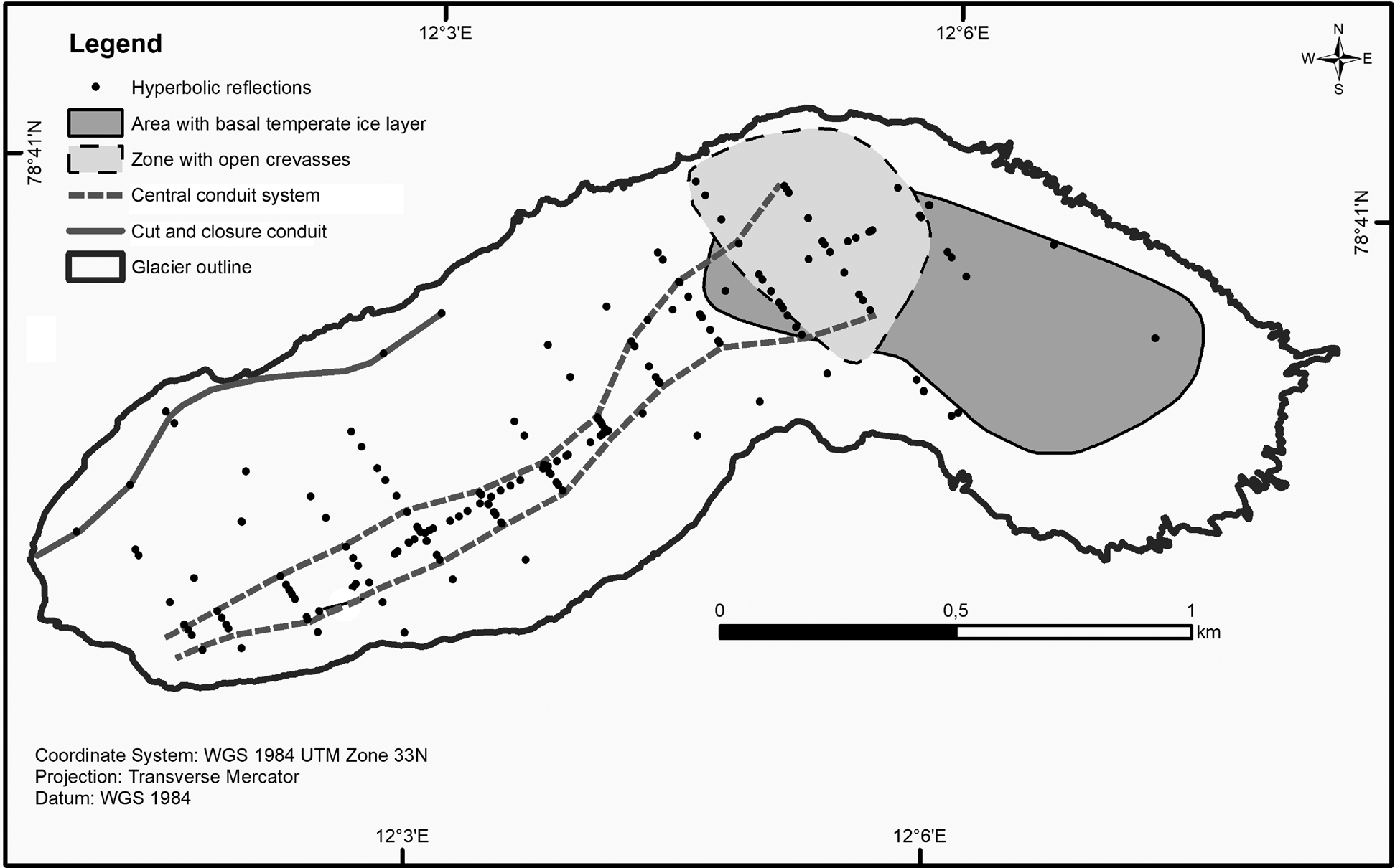
Fig. 10. Interpretation of the englacial drainage system at Waldemarbreen.
Most hyperbolic reflections associated with the ~120 m wide central system (Fig. 10) were confined vertically within cold-based glacier ice (Fig. 9). Numerous, closely spaced hyperbolic reflections were present (Fig. 10), whose variable amplitude might indicate the presence of abandoned sections of a major, meandering conduit (e.g. Hansen and others, Reference Hansen, Piotrowski, Benn and Sevestre2020). However, the spacing of the observed hyperbolae seems too wide (~120 m) for a single, meandering englacial conduit on a glacier this size. It is unclear, whether the features indicate either a long history of combined channel migration and abandonment in a single conduit, or the presence of multiple, smaller conduits concurrently following the same hydraulic gradient. As the amplitude of hyperbolic reflections varies greatly, the strongest reflections could be linked to active conduits that are at least partially filled with water, while the weakest reflections could probably be linked to small abandoned conduits that are filled with air (e.g. on Profile 5 reflections with varying amplitude can be seen in Fig. 8b). We base this assumption on the fact that the dielectric contrast between ice and water is much greater than that between ice and air (Jol, Reference Jol2009) as well as observations in previous studies (e.g. Karlsson and others, Reference Karlsson2019). If this is the case, then pressurisation was unlikely during our investigation in August, as is also discernible in the subglacial portal shown in Figure 11a, which we assume is the outflow from the central englacial system. The meltwater generation during this time period in western Svalbard is rather low due to freezing temperatures at night and even colder days. The differentiation between possibly active (at least partially filled with meltwater) conduits and abandoned ones however is not reliably accomplishable from GPR data and is not done in this study because many other variables not just dielectric contrast could lead to changes of amplitude as local variations of signal attenuation, size of the conduit, local increase of dielectric permittivity and conductivity of the glacier surface that would lead to changes of antenna radiation pattern.

Fig. 11. (a) Entrance of the glacier drainage system at the front of Waldemarbreen. (b) Outburst of pressurised subglacial water.
There are various mechanisms by which englacial conduits can form (for summaries see Gulley and others, Reference Gulley, Benn, Screaton and Martin2009a and Irvine-Fynn and others, Reference Irvine-Fynn, Hodson, Moorman, Vatne and Hubbard2011). We hypothesise that the hydrofracturing mechanism is most consistent with our observations of the central system at Waldemarbreen. The process was most likely initiated following sustained meltwater entry into the crevasses of the upper glacier. Hydrofracturing has been observed both in cases when surface meltwater propagates downwards to the glacier bed (Benn and others, Reference Benn, Gully, Luckman, Adamek and Glowacki2009; Bælum and Benn, Reference Bælum and Benn2011) and vice versa, when pressurised subglacial water forces a connection upwards to the surface of the glacier (Bingham and others, Reference Bingham, Nienow, Sharp and Boon2005). Fountain and others (Reference Fountain, Jacobel, Schlichting and Jansson2005) reported in situ creation of crevasses at a depth of 137 m in the polythermal Storglaciaren, while Benn and others (Reference Benn, Gully, Luckman, Adamek and Glowacki2009) observed that hydrologically driven fractures could form entirely englacially at Hansbreen, Svalbard. Bingham and others (Reference Bingham, Nienow, Sharp and Boon2005) and Skidmore and Sharp (Reference Skidmore and Sharp1999) described how pressurised subglacial water forced a path through cold ice and/or frozen sediments to cause artesian fountains close to the margin of the polythermal John Evans Glacier. Such outbursts were first described in Svalbard at Werenskiöldbreen by Baranowski (Reference Baranowski1973), and later linked to drainage network initiation at Midtre Lovénbreen by Hodson and others (Reference Hodson, Kohler, Brinkhaus and Wynn2005). Their occurrence at Waldemarbreen and nearby glaciers has been documented regularly for the period 1996–2015, especially during late winter (Sobota, Reference Sobota2016), and also during the present study in summer (August 2019) (Fig. 11b). At the end of the 1960s, temporary winter meltwater outflow was observed on the glacier at 25 m from its margin, forming supraglacial icings (Grześ and Sobota, Reference Grześ and Sobota2000). We, therefore, argue that pressurisation has the capacity to induce hydrofracturing through the cold ice region of Waldemarbreen. The sub-horizontal orientation of the central englacial system is also in accordance with observations from elsewhere, since Irvine-Fynn and others (Reference Irvine-Fynn, Hodson, Moorman, Vatne and Hubbard2011) described how conduits formed via hydrofracturing can become inclined at progressively shallower angles in a down-glacier direction. Mavlyudov (Reference Mavlyudov and Mavlyudov2005) directly observed entirely horizontal hydrofractures that later developed into separate conduits while the rest of the crevasse closed.
Alternative would be the cut and closure mechanism (Fountain and Walder, Reference Fountain and Walder1998) that is believed to be one of the main mechanisms for conduit formation in polythermal and cold glaciers in Svalbard (Gulley and others, Reference Gulley, Benn, Müller and Luckman2009b) and since they develop on glaciers where channel incision rates exceed ablation rates, a large catchment area tends to be the main pre-requisite (Gulley and others, Reference Gulley, Benn, Screaton and Martin2009a). A low incidence of crevassing is particularly important for enabling large catchment areas, and we point out that, while the glacier surface in the ablation zone is relatively crevasse free, the central englacial system can be clearly traced back to the crevassed region of the upper glacier (Figs 2a, b). The orientation of supraglacial streams does not coincide with the orientation of our proposed englacial conduit system. All streams at the southern part of the glacier flow obliquely towards its lateral margin (Fig. 3) and we would expect a cut and closure system to follow a similar course. Furthermore, cut and closure conduits usually generate slightly offset-stacked hyperbolae, as reported by Bælum and Benn (Reference Bælum and Benn2011) and Teminghoff and others (Reference Temminghoff, Benn, Gulley and Sevestre2018), while at Waldemarbreen, we observed a single hyperbola in most cases.
At the northern lateral margin of the glacier, we identified single-hyperbolic reflections on several B-scans (Fig. 10) that were aligned with another subglacial portal at the margin. Although these hyperbolic reflections could also be theoretically related to large rocks, we observed two supraglacial streams in this part of Waldemarbreen that were incised down into the ice and could potentially form cut and closure conduits in the future (Fig. 2b). This observation showed that such a process could have also been effective in the past. Cut and closure conduits are very common along the margins of small cold-based glaciers in Svalbard, as exemplified by a detailed study of Tellbreen (Naegeli and others, Reference Naegeli, Lovell, Zemp and Benn2014). While the evidence for cut and closure conduits in the northern margin of the glacier is more compelling, crevasse traces in the same area mean that other conduit formation processes might still have initiated (or further contributed to) conduit evolution. Direct speleological observations in the englacial conduits at Waldemarbreen could, therefore, further clarify the morphology and origin of Waldemarbreen's drainage system.
Alternative explanations for observed hyperbolae seem implausible. First, such reflections could be related to longitudinal crevasses, but we exclude this possibility because we did not map any longitudinal crevasses or crevasse traces on the surface of Waldemarbreen. Second, the observed reflections could be related to boulders, but since no medial moraine is present it is rather difficult to explain why individual boulders would be aligned at specific depth intervals in the middle part of the glacier (Figs 9 and 10).
Conclusions
GPR measurements clearly reveal a polythermal structure at Waldemarbreen. The glacier is predominantly cold with temperate ice in its upper reaches. The thickness of temperate ice reaches at least 80 m, and this layer is ~40 m thick on average. The maximum detected ice thickness reaches ~140 m in the accumulation area, although the glacier is slightly thicker, as we were not able to detect reflections from the glacier bed at its deepest part.
The existence of the basal temperate ice layer at Waldemarbreen cannot be explained as only a function of the contemporary ice thickness because it coincides with an ice thickness of just ~40 m in the up-glacier area. Here, the temperate ice can be viewed as a relict phenomenon formed in the past when lower ELAs and crevasses allowed stored water to freeze and release latent heat. Today, it is likely that only refreezing in crevasses can contribute to this release of heat, although this will be minimal while the two observed moulins persist. High modern ELAs mean that insulation and latent heat associated with firn refreezing in the accumulation area no longer play a meaningful role in the generation of temperate ice. The glacier, therefore, lacks thermal equilibrium with the current climate and is cooling. The upper surface of the temperate ice, now 20 m below the glacier surface, is likely to get deeper as the glacier equilibrates via heat loss in winter.
Asymmetry in the cross-glacier subglacial topography was observed, including a subglacial mound with dimensions of ~240 m × 200 m × 7 m and comprised of unconsolidated gravel/pebble-rich sediments in the mid-ablation area, as well as an off-centre subglacial trough between the glacier centre line and its southern lateral margin. Here, multiple reflection hyperbolae were found in GPR profiles, suggesting the presence of a major englacial drainage system within cold ice. The depth from the glacier surface to the observed conduits increases up-glacier and can be traced to the temperate zone in the upper glacier.
It has been suggested that cut and closure is the dominant formation mechanism for low-gradient englacial conduits on uncrevassed regions of polythermal glaciers and probably the only likely mechanism for cold ice. However, we propose hydrofracturing, rather than cut and closure, as the main mechanism in the development of the englacial system at Waldemarbreen. The importance of hydrofracturing through high-elevation crevasses is most likely under-appreciated in the context of polythermal glaciers, largely due to their high-elevation location. We argue that more attention needs to be directed towards these features in parts of the Arctic such as Svalbard where loss of firn from (former) glacier accumulation areas is now occurring. The firn loss makes the conditions for hydrofracture more favourable because it promotes more rapid drainage of meltwater and rainfall into the crevasses.
Acknowledgements
Research was funded by the Latvian Council of Science, project ‘Thermal structure, drainage system and surface changes of Kaffiøyra Region glaciers, north-western Svalbard’, project No. lzp-2020/2-0279, by the specific support objective activity 1.1.1.2, ‘Post-doctoral Research Aid’ (Project id. 1.1.1.2/16/I/001) of the Republic of Latvia, funded by the European Regional Development Fund, Kristaps Lamsters research Project No. 1.1.1.2/VIAA/1/16/118, the performance-based funding of the University of Latvia within the ‘Climate change and sustainable use of natural resources’ programme and it was carried out as part of the ‘Changes of north-western Spitsbergen glaciers as the indicator of contemporary transformations occurring in the cryosphere’ (2017/25/B/ST10/00540) project funded by the National Science Centre, Poland. The authors thank all other members of the Nicolaus Copernicus University expedition to Svalbard in 2019 for their assistance in fieldwork and anonymous reviewers for constructive remarks, which helped to strengthen and focus the manuscript. We also thank scientific editor B. Kulessa and reviewers for many valuable suggestions that greatly improved the manuscript.


 Open access