


1. Introduction
Himalayan glaciers are shrinking and losing mass at rates comparable to the other regions of the globe (Bolch and others, Reference Bolch2012; Azam and others, Reference Azam2018; Hock and others, Reference Hock, Pörtner, Roberts, Masson-Delmotte, Thai, Tignor, Poloczanska, Mintenbeck, Alegría, Nicolai, Okem, Petzold, Rama and Weyer2019; Hugonnet and others, Reference Hugonnet2021). The ice loss has clearly increased after 2000 which can mainly be attributed to the current phase of accelerated atmospheric warming in the region (Sakai and Fujita, Reference Sakai and Fujita2017; Bolch and others, Reference Bolch, Wester, Mishra, Mukherji and Shrestha2019; King and others, Reference King, Bhattacharya, Bhambri and Bolch2019; Maurer and others, Reference Maurer, Schaefer, Rupper and Corley2019; Bhattacharya and others, Reference Bhattacharya2021). Recent projections indicate that, depending on the climate scenario, Himalayan glaciers will lose between 30 and 60% of their current mass by the end of the 21st century (Kraaijenbrink and others, Reference Kraaijenbrink, Bierkens, Lutz and Immerzeel2017; Rounce and others, Reference Rounce, Hock and Shean2020). This will adversely affect the run-off in the major river systems of High Mountain Asia (Bolch, Reference Bolch2017; Immerzeel and others, Reference Immerzeel2020; Azam and others, Reference Azam2021), particularly during periods and years with low precipitation (Pritchard, Reference Pritchard2019).
Remote-sensing and field-based measurements indicate that the glacier changes are variable throughout the Himalaya (Scherler and others, Reference Scherler, Bookhagen and Strecker2011; Kulkarni and Karyakarte, Reference Kulkarni and Karyakarte2014; Azam and others, Reference Azam2018). The general behaviour of the glaciers is driven by climate, primarily by temperature and precipitation (Oerlemans and others, Reference Oerlemans1998; Oerlemans, Reference Oerlemans2005). However, the individual glacier response to the climatic forcing is strongly controlled by non-climatic factors determined by topography and the extent of debris cover (Salerno and others, Reference Salerno2017; Bush and Bishop, Reference Bush and Bishop2018). Consequently, two neighbouring basins that experience a similar regional climate could respond quite differently to climate forcing due to differences in the topographic settings (Garg and others, Reference Garg, Shukla and Jasrotia2017). It is therefore important to assess the influence of climatic and topographic parameters on the glacier changes at basin scale. In this paper, we concentrate on the Upper Alaknanda Basin (UAB) in the Central Himalaya where such investigations are limited and no detailed up to date glacier inventory and estimates of glacier area change exist. A basin scale glacier inventory is available for the year 2006 and area changes were estimated for the period between 1968 and 2006 (Bhambri and others, Reference Bhambri, Bolch, Chaujar and Kulshreshtha2011a). The present study focuses on the period from 2006 onwards. The previous work done in the UAB is reviewed below.
Bhambri and others (Reference Bhambri, Bolch, Chaujar and Kulshreshtha2011a) generated a glacier inventory of 83 glaciers in the basin for the year 2006 and reported an area loss of 5.7 ± 2.7% (0.14 ± 0.06% a−1) from 1968 to 2006. Surface elevation changes of glaciers of UAB have been recently reported from 2000 to 2014 (Bandyopadhyay and others, Reference Bandyopadhyay, Singh and Kulkarni2019) and for the period 2000–2017 by Remya and others (Reference Remya, Kulkarni, Hassan and Nainwal2020). Both studies indicate an almost similar mean surface lowering, 0.37 m a−1 (2000–2014) and 0.33 m a−1 (2000–2017). Based on simple models validated with limited field data, the ice volume of the basin has been estimated to be 26.4 km3 for the year 2016 (Mishra and others, Reference Mishra, Nainwal, Dobhal and Shankar2021).
There have been several studies of the larger glaciers in the basin. Field studies on Satopanth and Bhagirath Kharak glaciers by Nainwal and others (Reference Nainwal2007) report three phases of glaciation in the valley during late quaternary period. Nainwal and others (Reference Nainwal, Negi, Chaudhary, Sajwan and Gaurav2008) have estimated the length and area changes for Satopanth glacier to be 22.8 m a−1 and 0.314 km2 and for Bhagirath Kharak glacier to be 7.42 m a−1 and 0.13 km2 between 1962 and 2005. Nainwal and others (Reference Nainwal, Banerjee, Shankar, Semwal and Sharma2016) have extended this analysis to the period 1937–2013 and reported retreat rates to be 5.7 and 6.0 m a−1 for Satopanth and Bhagirath Kharak glaciers respectively, corresponding to the area loss of 0.27 and 0.17 km2. Mishra and others (Reference Mishra, Negi, Banerjee, Nainwal and Shankar2018) conducted ground-penetrating radar measurements and found the average ice thickness in the snout and upper ablation regions to be 40 and 100 m, respectively. Shah and others (Reference Shah, Banerjee, Nainwal and Shankar2019) have reported sub-debris ice melt variability (1.5–1.7 cm d−1) during 2015–17 based on the glaciological method. A modelling study on Satopanth Glacier to quantify the avalanche contribution in glacier mass balance shows that ~90% of the total glacier mass gain (~1.8 m w.e. a−1) is dominated by avalanches (Laha and others, Reference Laha2017). Remya and others (Reference Remya, Kulkarni, Hassan and Nainwal2020) found significant mass loss (0.55 ± 0.06 m w.e. a−1) of Satopanth glacier during 2000–2017 as compared to 0.09 ± 0.04 m w.e. a−1 1962–2000. Moreover, Garg and others (Reference Garg, Shukla and Jasrotia2017) have reported the results of a remote-sensing study on changes of length (~5–30 m a−1) and area (~2.2%) of four glaciers of the UAB, during 1994–2015. Shukla and Garg (Reference Shukla and Garg2020) have further estimated the spatio-temporal changes in the surface ice velocities of these glaciers. The study shows consistent reduction of average surface ice velocity from 22.6 m a−1 (1993–94) to 17.3 m a−1 (2000–01) and further decrease to 11.5 m a−1. These previous studies, however, do not assess the characteristics of the individual glaciers in the basin. Furthermore, no study in the UAB has investigated area changes after 2006 including all the glaciers in the basin.
The objective of this work is to extend the current knowledge about the UAB by (i) generating a glacier inventory for 2020 including topographic parameters, snow line altitude and debris cover extent, (ii) estimating changes in area, length and debris cover area during the period 1994–2020 and (iii) correlating glacier area changes with climate and glacier-specific characteristics. We do this to contribute to the understanding of the complex processes of the dynamics of the collection of glaciers in the UAB in a rapidly changing climate.
2. Study area
Our study area, the UAB is located in the Central Himalayan region in Uttarakhand, a northern Indian state (Fig. 1). It is located between the latitude and longitude of 30.5–31°N and 79.25–79.72°E respectively. The Alaknanda River originates from the ~13 km long and ~750 m wide Satopanth Glacier (snout ~3880 meter above sea level [m a.s.l.]). UAB is a part of the Alaknanda Basin classified by the Geological Survey of India (GSI) as a third-order basin (5O 132) of Ganga River. The Alaknanda Basin has ~400 glaciers with an area of ~1200 km2 (Raina and Srivastava, Reference Raina and Srivastava2008). It contains all glaciers that contribute to the Alaknanda River after confluence with the Dhauliganga River at Vishnuprayag (Fig. 1). The UAB contains all glaciers that contribute to the Alaknanda River before its confluence with the Dhauliganga. The river system of UAB has a general orientation in north-south direction and its river tributaries and sub-catchments mostly have an east-west trend. The basin covers an area of ~1500 km2 and ranges from ~1450 m (Vishnuprayag) to 7756 m a.s.l. (Kamet). Chaukhamba (~7138 m a.s.l.) is the second highest peak in the basin and the source of several large glaciers such as Satopanth, Bhagirath Kharak on the eastern and the north-eastern slopes and the Gangotri group of glaciers on the western slopes (Fig. 1).

Fig. 1. Location map of the study area showing clean and debris-covered parts of the glaciers and main localities. Inset (a) Uttarakhand State and footprints of the satellite images used in the study, (b) climate diagram (1901–2019) for the basin extracted from CRU data. The numbers (1–20) indicate glaciers with length change estimations. The star shows the field surveyed snout locations of Satopanth (2) and Bhagirath Kharak (3) glaciers.
A significant fraction of the glacierised area of the basin is debris-covered. Bhambri and others (Reference Bhambri, Bolch, Chaujar and Kulshreshtha2011a) report ~25% of the glacierised area being debris-covered. Field measurements on the Satopanth glacier (Shah and others, Reference Shah, Banerjee, Nainwal and Shankar2019) indicate that while the debris thickness decreases with elevation, there is a large spatial variation. The debris is mainly composed of kyanite-sillimanite schist, gneisses and leucogranites which belong to the Pandukeshwar and Pindari Formations (Valdiya and others, Reference Valdiya, Paul, Chandra, Bhakuni and Upadhyay1999).
The Central Himalaya receives most of its precipitation from the Indian summer monsoon. However, contribution from the westerlies in the region is also significant (Bookhagen and Burbank, Reference Bookhagen and Burbank2006; Thayyen and Gergan, Reference Thayyen and Gergan2010). There are no instrumental climatic records available in the UAB. The Indian Meteorological Department (IMD) operates a weather station at Joshimath (~1650 m a.s.l.) located a little south of the basin. Measurements recorded mean annual precipitation of ~1100 mm from the period 1959–2013 (Kumar and others, Reference Kumar, Mehta, Mishra and Trivedi2017). The ambient mean monthly temperature from June was 29°C and that in October was ~5°C.
The Climate Research Unit (CRU) TS 4.04 data for the study area shows mean monthly temperatures varying from ~−7°C in January to ~11°C in July during 1901–2019 (Fig. 1b). The long-term mean monthly precipitation data show that maximum precipitation in UAB occurs during summer from June to September. The highest precipitation is recorded in the month of July (~151 mm) and August (~148 mm) followed by September (~83 mm) and June (~73 mm) (Fig. 1b). The mean annual air temperature and precipitation of the UAB for the period 1901–2019 were 2.2°C and ~700 mm, respectively. The summer precipitation contributed ~75% to the total annual precipitation.
3. Methodology
3.1. Data
We used different multi-temporal remote-sensing data 1994–2020 for glacier mapping detailed in Table 1. Satellite images of the ablation period (i.e. September and October) with minimum seasonal snow and cloud cover were selected. The Sentinel-2A image of 8 October 2020 was used as a reference image as it had most suitable conditions and matched best with our field-based differential GPS (DGPS) mapping over the frontal parts of Satopanth and Bhagirath Kharak glaciers conducted 6–7 October 2020 (Fig. 2). Two further Sentinel-2A images (acquired 13 September 2020 and 18 October 2020) were also checked to discard snow patches and misclassified shadow zones. The satellite data from the different sensors were co-registered with the Sentinel-2A images as a master image using the projective transformation algorithm in ERDAS Imagine 2014 (cf. Bolch and others, Reference Bolch2010a; Frey and others, Reference Frey, Paul and Strozzi2012). In total, 32 common control points, such as confluences of streams, intersections of streams and roads, ‘crossed ridges’, and prominent peaks and moraines were selected to assess the horizontal accuracy. We assumed that no changes in these features had occurred. The common points were distributed throughout the study area with the highest concentration around the glacierised regions. We could achieve a root mean square error (RMSE) less than the pixel size of the images, i.e. ~16 m for TM and ~13 m for ASTER scenes. While the ASTER image has a relatively higher RMSE value and limited study area coverage, we used it in our study to compare the results of the previous study in UAB by Bhambri and others (Reference Bhambri, Bolch, Chaujar and Kulshreshtha2011a). A short wave infrared (SWIR) band is needed for automated glacier mapping owing to the distinctive reflectance and absorption properties of snow and ice as compared to visible and near infrared (NIR) bands (Paul and others, Reference Paul2015). The SWIR bands of ASTER (band-4) and Sentinel (band-12) images have lower spatial resolutions of 30 and 20 m respectively, and were therefore resampled in ERDAS Imagine 2014 to 15 and 10 m, respectively, to match the resolution of the visible and NIR bands of the ASTER and Sentinel-2A images.
Table 1. Details of the satellite data and digital elevation model (DEM) used in this study

TM, thematic mapper, NIR, near infrared; SWIR, shortwave infrared.

Fig. 2. Field photographs showing (a) the snout of Satopanth Glacier mapped with the help of DGPS on 7 October 2020, (b, c) the presence of dead ice mound, water pond and outwash plan in the vicinity of Satopanth Glacier, (d) the frontal part of Bhagirath Kharak Glacier (mapped on 6 October 2020) and associated dead ice (photos: A. Mishra 2020).
To extract the topographic information of the glaciers, the High Mountain Asia Digital Elevation Model (HMA DEM) (Shean, Reference Shean2017) was used (Table 1). This DEM was in particular generated based on high-resolution WorldView images acquired during 2013 and 2016 and has a spatial resolution of 8 m.
We used the HMA DEM due to its better spatial resolution as compared to the SRTM DEM and ASTER GDEM for the best temporal fit to the Sentinel-2 data. The problem with HMA DEM is the occurrence of few data voids, especially in areas with very low correlation in the optical stereo imagery used, e.g. near steep slopes or cast shadows. To obtain full coverage, we interpolated these voids using nearest neighbour interpolation. Since the glacierised areas were free from data gaps and the purpose of the DEM was extract topographic parameters, the voids did not impact the results of our study.
3.2. Glacier mapping
To map the glacier boundaries on the basis of satellite images, the recommendations of Global Land Ice Measurements from Space (GLIMS) initiative were followed (Paul and others, Reference Paul2009, Reference Paul2015; Racoviteanu and others, Reference Racoviteanu, Paul, Raup, Khalsa and Armstrong2009). The extents of glaciers were manually delineated on-screen in ArcGIS 10.5 with an approximate scale of 1 : 10 000 using different band combinations, for example, NIR-Red-Green, SWIR-NIR-Red, Red-Blue-Green (Fig. 3). We preferred manual mapping as many of the glaciers in our study are debris-covered for which the automated methods fail or have a low accuracy due to similar spectral properties of the surrounding debris (Bhambri and others, Reference Bhambri, Bolch, Chaujar and Kulshreshtha2011a; Frey and others, Reference Frey, Paul and Strozzi2012).

Fig. 3. Manually demarcated glacier outlines, (a, d) 1994 Landsat TM (1994), (b, e) ASTER (2006) and (c, f) Sentinel-2 (2020) images showing no visible changes in the upper regions of the glaciers.
The visual identification of the boundary of debris-covered glaciers is a challenging task particularly in the frontal regions (Bolch and others, Reference Bolch2010a; Paul and others, Reference Paul2013). The boundaries in these regions were identified considering colour differences and the surrounding geomorphology, such as steep ice walls or exposed ice faces, stream emerging points, outwash plains, lateral morainic ridges, water ponds and ice cliff shadows. The surface slope and shaded relief maps derived from the HMA DEM were used as additional information (Bolch and others, Reference Bolch, Buchroithner, Kunert and Kamp2007; Bhambri and others, Reference Bhambri, Bolch and Chaujar2011b). The presence of dead ice mounds creates another difficulty in delineation of debris-covered glaciers because of their close vicinity to the glacier fronts. Hence, high-resolution (~0.5–2.5 m) images available in Google Earth were taken as additional information along with the presence of surface meltwater ponds which differ from supraglacial ponds by their different reflectance caused by different turbidity. Also, our field experience at Satopanth and Bhagirath Kharak glaciers (Fig. 2) helped us to delineate glacier boundaries especially near the glacier fronts.
The glacier inventory was prepared based on the 2020 Sentinel image with the smallest glacier area of a glacier being 0.02 km2. A similar size threshold was used for the Himalayan glacier inventory by ICIMOD (Bajracharya and Shrestha, Reference Bajracharya and Shrestha2011) and, in Western Himalaya, by Frey and others (Reference Frey, Paul and Strozzi2012). The distinction between snow patches and small glaciers (<0.5 km2) is crucial, since snow can accumulate for few years on mountain slopes and ridges. We excluded such seasonal snow patches by a visual interpretation of the additional Sentinel-2 images (Table 1) and high-resolution images of Google Earth along with field studies around Satopanth Glacier. For the glacier inventory, contiguous ice masses were separated into glaciers based on the HMA DEM, using hydrologic functions in ArcGIS and further checked and adjusted using shaded relief map and Google Earth 3-D views (Racoviteanu and others, Reference Racoviteanu, Paul, Raup, Khalsa and Armstrong2009; Bolch and others, Reference Bolch, Menounos and Wheate2010b; Das and Sharma, Reference Das and Sharma2018).
The late summer snowline altitude (SLA) was retrieved for the glacier inventory (2020) by manually delineating the snowline using the band combination SWIR (12)-NIR (8)-Green (3) of the master Sentinel-2 image (cf. Rabatel and others, Reference Rabatel, Dedieu and Vincent2005; Shukla and others, Reference Shukla, Garg, Mehta, Kumar and Shukla2020). A buffer of 15 m was created on either side of the marked snowline and mean altitude of this buffer zone was extracted using the HMA DEM.
3.3. Quantification of glacier-specific characteristics
The mapped glaciers were classified based on their area and morphology. The coarse area ranges chosen were <0.5; 0.5–1; 1–5; 5–10; >10 km2. The glaciers were categorised as valley and mountain glaciers, according to the GLIMS guidelines (Rau and others, Reference Rau, Mauz, Vogt, Khalsa and Raup2005). Valley glaciers have well-defined accumulation and ablation areas and their form is controlled by the respective topography. Such glaciers follow pre-existing valley-shapes and are further divided into compound and simple basin. The remaining glaciers are those which lie on mountain slopes and terminate before reaching the main valley. Such glaciers are defined as cirque glaciers, hanging glaciers and mountain glaciers (Fig. 4).

Fig. 4. Example of the morphological classification of glaciers of UAB mapped from Sentinel images (Hillshade map in the background): (a) simple basin, (b) cirque, (c) compound basin, (d) mountain glaciers, (e) hanging glacier, (f) field photograph of the hanging glacier (e) taken during fieldwork in 2016 (photo: A. Mishra 5 September 2016).
The glacier outlines and the DEM enabled us to extract the elevation parameters of the glacier surface. Glacier area, perimeter, minimum, maximum and mean elevations, the elevation range and the mean slope of each glacier were extracted using zonal statistical tools in ArcGIS. Glacier lengths were calculated from manually drawn centre-lines. The aspect was calculated on the basis of the orientation of the centre-lines. In case of arc-shaped glaciers, the average direction of the trunk glacier was taken to determine the aspect.
3.4. Change detection analysis
Area changes of 138 glaciers were estimated for the periods 1994–2006 and 2006–2020. We could not map the area changes of all 198 glaciers of the 2020 inventory since not all of them were clearly visible in the Landsat image owing to partial cloud cover and limited coverage of the 2006 ASTER image. In total, 175 glaciers could be investigated for the period 1994–2020.
To calculate the glacier area-changes, the glacier-boundaries demarcated in the ‘base image, 2020’ were superimposed over the previous glacier-boundaries (cf. Bolch and others, Reference Bolch2010a, Reference Bolch, Menounos and Wheate2010b). The upper parts of the glacier showed no measurable changes during the study period (as also noted by Bhambri and others, Reference Bhambri, Bolch, Chaujar and Kulshreshtha2011a), except around the internal rocks. Therefore, area changes were mainly in the vicinity of the fronts (Fig. 3). Several glaciers fragmented during the study period; in such cases, the total fragmented area was used to estimate the area change.
We calculated the length changes of selected UAB glaciers for both the periods (i.e. 1994–2006 and 2006–2020). The glaciers were selected on the basis of their frontal morphology: a well-defined glacier front and confined by lateral moraines and a straight and narrow glacier tongue. As most of the small glaciers (<5 km2) in UAB have irregular fronts we discarded them and finally 20 larger glaciers (numbered 1–20 in Fig. 1) were chosen for length change measurements. The glacier-boundaries from the different years were superimposed over each other. For the estimation of glacier retreat, parallel lines were drawn on either side of the central flow-line (or along the maximum glacier length) at 50 m intervals (Supplementary Fig. S1); and the changes in length along each of these lines were then averaged (cf. Koblet and others, Reference Koblet2010; Bhambri and others, Reference Bhambri, Bolch and Chaujar2012).
4. Uncertainty estimations
The uncertainties of the glacier boundaries were estimated in two ways: (a) by comparing the glacier outlines from the satellite image (2020) to a field survey done during the same period at Satopanth and Bhagirath Kharak glaciers, and (b) using the buffer method (Granshaw and Fountain, Reference Granshaw and Fountain2006; Bolch and others, Reference Bolch2010a; Chand and Sharma, Reference Chand and Sharma2015). The boundaries of Satopanth and Bhagirathi Kharak glacier fronts (Fig. 2) were mapped by a DGPS survey, having horizontal accuracy of ±10 cm. The difference between the surveyed DGPS points and the manually mapped boundaries over two glaciers was ~5 m at the front ice cliff regions and ~8–12 m at the debris-covered parts (Fig. 5).

Fig. 5. Satopanth and Bhagirath Kharak glacier boundaries mapped by DGPS data in 2020 and manually demarcated glacier boundary (blue) based on the Sentinel-2 image (SWIR-NIR-Red) of the same year.
To estimate the area uncertainties of all glaciers, the buffer method was used with buffer sizes of half of the pixel size or co-registration error between two images. These were 5, 6.5 and 8 m for the Sentinel-2, ASTER and Landsat TM images respectively. This resulted in an average mapping uncertainty of 3.5% for TM, 2.75% for ASTER and 2.3% for Sentinel-2. These estimates are consistent with the previously reported mapping uncertainties (Bolch and others, Reference Bolch2010a; Bhambri and others, Reference Bhambri, Bolch, Chaujar and Kulshreshtha2011a; Paul and others, Reference Paul2013; Chand and Sharma, Reference Chand and Sharma2015; Garg and others, Reference Garg, Shukla and Jasrotia2017). The uncertainty in area changes was estimated according to the standard error propagation, as root sum square of the uncertainty for outlines mapped from different sources (Bhambri and others, Reference Bhambri, Bolch, Chaujar and Kulshreshtha2011a).
The length uncertainty of the three satellite images of different years was estimated by considering the following equations (Hall and others, Reference Hall, Bayr, Schöner, Bindschadler and Chien2003):

where ‘a’ and ‘b’ are spatial resolution of the images 1 and 2, respectively, and σ is the co-registration error which was 16 m in case of Landsat TM (1994) and 13 m for ASTER (2006). The resultant length change uncertainty was found to be 47.6 m TM and 31.0 m for ASTER.
5. Temperature and precipitation data
CRU data (version 4.04) (Harris and others, Reference Harris, Osborn, Jones and Lister2020) from 1901 to 2019 was used for the analysis of temperature and precipitation. The study area is located within two 0.5 degree grids (Fig. 1): grid 01 (30.75°N, 79.25°E) and grid 02 (30.75°N, 79.5°E). The trend was similar for these two grid points. Thus, we have averaged the two datasets. A statistical analysis shows that the averaging of both the grids does not affect the trend in the data (Supplementary Table S1). A non-parametric Mann–Kendall test was used to determine the statistical significance of the trend, and the magnitudes of the trend were obtained through a linear regression analysis (Bhambri and others, Reference Bhambri, Bolch, Chaujar and Kulshreshtha2011a). The trend analysis has been done on annual basis.
6. Results
6.1. Glacier inventory
The 2020 inventory of the study area comprises 198 glaciers of different sizes, morphological types and extents of debris cover (Tables 2 and 3; Fig. 6). The total glacierised area is 354.6 ± 8.1 km2, of which ~27% is covered with debris. Out of the 198 glaciers, 64 were debris-covered. While only 10 of the 198 glaciers have an area of more than 10 km2, they occupy ~50% of the total glacierised area. The large glaciers tend to have compound basins; consequently about half the glacierised area is in compound basins. Of the morphological types the number of mountain glaciers is the highest (Fig. 7).

Fig. 6. The distribution of glaciers of UAB: (a) based on their size and (b) based on their morphology.

Fig. 7. Distribution of number of glaciers, total glacierised area and mean slope for each area range and morphological type.
Table 2. Glacier parameters of different area ranges

Table 3. Glacier parameters of different morphological types

The area-elevation distribution shows that ~50% of the area is located at the elevation ~5200 m a.s.l. (Fig. 8a). However, the area of the large glaciers (>10 km2) is much more broadly distributed in the elevation range 4700–5800 m a.s.l., consistent with debris-covered glaciers which tend to have long narrow tongues. The debris-covered area is broadly distributed between 3800 and 5850 m a.s.l. There are two prominent peaks of debris-covered extents at an elevation of 4350 and 5100 m a.s.l. This may be due to the location of snouts of large debris-covered glaciers at higher altitude. For example, the snout of Balabala Glacier (No-12 in Fig. 1) is located at an elevation of ~5040 m a.s.l. which is significantly higher than the glaciers (i.e. Bhagirath Kharak) having minimum elevations (~3880 m a.s.l.). The most frequent glacier aspect is north (n = 41), followed by south (n = 39), while glaciers facing southeast (65.2 ± 2.3 km2) and southwest (63.2 ± 2.2 km2) have the greatest area (Fig. 8b).

Fig. 8. (a) Area-elevation distribution of all glaciers (blue) and of the glaciers in different size ranges (other colours). (b) Distribution of glacier number and glacierised area at different orientations. (c) Debris-covered area plotted against the total glacier area.
The snowline of the UAB glaciers is located at an elevation of ~5300 m a.s.l. with glaciers between 5 and 10 km2 having the highest average snowline of 5467 m a.s.l. The SLA of large glaciers (>10 km2) is located at a slightly lower elevation (5352 m a.s.l.) probably due to their large elevation range and low lying tongues. The glaciers <0.5 km2 and of 0.5–1.0 km2 in size have the SLA at a similar elevation of 5262 and 5254 m a.s.l., respectively. The hanging glaciers have a relatively higher mean slope (27°) than the mountain glaciers (24°). The mean slope is 24° which varies from 16° to 26° in >10 and <0.5 km2 glacier sizes, respectively.
The extent of debris cover increases with the increasing size of the glacier. Large glaciers (>10 km2) have ~35% of their area covered with debris; whereas the smaller glaciers (<0.5 km2) are almost debris-free. In fact only 65 of the 198 glaciers had debris cover in 2020. Most of the debris-free glaciers are of <1 km2 in size (Fig. 8c).
6.2. Area changes
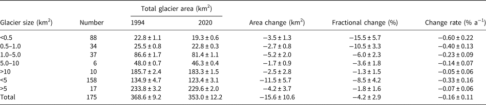
The glacierised area of the basin has reduced from 368.6 ± 9.2 km2 in 1994 to 353.0 ± 5.3 km2 in 2020, a change of 4.2 ± 2.9% (0.16 ± 0.11% a−1) (Table 4). The area loss of individual glaciers varied from 0.5 ± 0.8 to 38 ± 3.9% between 1994 and 2020. The relative area loss (%) has been grouped in six classes (<5; 5–10; 10–15; 15–20; 20–25 and >25) and geographical distribution (Fig. 9). The number of glaciers increased from 175 to 198 during the period of study due to fragmentation. The relative % area loss of small glaciers (<5 km2) was ~8.5%, which was significantly larger than that of the large (>5 km2) glaciers (~1.8%) from 1994 to 2020. Very small glaciers (<0.5 km2) lost ~15% of their area. In terms of the glacier morphology, mountain glaciers experienced the highest area losses (10.6%), followed by hanging glaciers (~9.2%) and cirque glaciers (~8.6%) (Supplementary Table S2). Out of the 175 glaciers analysed for area change during 1994–2020, 113 were debris-free. During this period, the total area of debris-covered glaciers reduced from 305.3 ± 7.6 to 296.6 ± 4.4 km2 corresponding to 2.9 ± 2.9% (0.11 ± 0.11% a−1) whereas the relative area loss of the debris-free glaciers was 10.8 ± 2.8% (0.42 ± 0.11% a−1).

Fig. 9. The distribution of the area loss of 175 glaciers in the basin during the period 1994–2020.
Table 4. Area loss of 175 glaciers from 1994 to 2020 according to their size
The area changes of 138 glaciers were analysed for the periods 1994–2006 and 2006–2020. The total area of these glaciers was 332.4 ± 8.3 km2 in 1994, 326.8 ± 6.9 km2 in 2006 and 319.5 ± 4.8 km2 in 2020. Hence, the total area change during the periods was −1.7 ± 3.2% (−0.14 ± 0.27% a−1) during 1994–2006, and −2.2 ± 2.6% (−0.16 ± 0.19% a−1) during 2006–2020. While the mean value of the area loss has slightly increased in the period 2006–2020 as compared to 1994–2006, no significant trend can be inferred.
6.3. Length changes
The length of all 20 glaciers studied decreased during the period 1994–2020 with an average retreat rate of 11.4 ± 1.8 m a−1. The retreat rate of individual glaciers varied considerably between 4.6 ± 1.8 m a−1 (Arwa 01 Glacier) and 18.9 ± 1.8 m a−1 (Khuliya Garvya Glacier) (Fig. 10). The average retreat rate of the 18 glaciers which are covered in all the three scenes was 9.6 ± 1.9 m a−1 during 1994–2006 and 14.9 ± 1.2 m a−1 during 2006–2020. For two of the 18 glaciers, the retreat rate increased during 2006–2020 as compared with that of 1994–2006. The retreat rate of Bhagirath Kharak (glacier number 3 in Fig. 1) increased quite significantly from 4.9 ± 1.9 m a−1 during 1994–2006 to 16.0 ± 1.2 m a−1 during 2006–2020. Thus, it can be inferred that the retreat rate of the large glaciers in the basin has significantly increased in the period 2006–2020 as compared to 1994–2006.

Fig. 10. Retreat rates of the 20 investigated glaciers for the periods 1994–2006, 2006–2020 and 1994–2020. For numbering see Figure 1.
6.4. Debris cover changes
The debris-covered area of the studied 175 glaciers increased from 80.1 ± 2.8 km2 in 1994 to 90.8 ± 2.2 km2 in 2020, corresponding to a rate of increase of 0.52 ± 0.17% a−1. For the 138 glaciers measured in 1994, 2006 and 2020, the debris cover increased from 65.1 ± 2.3 km2 (21.0%) in 1994 to 67.5 ± 1.9 (21.8%) in 2006 to 73.3 ± 1.8 km2 (24.7%) in 2020. The percentage of increase corresponding to the debris cover was 0.31 ± 0.38% a−1 (1994–2006), 0.61 ± 0.27% a−1 (2006–2020) and 0.49 ± 0.17% a−1 for the whole study period (1994–2020). Thus, the rate during 2006–2020 was significantly larger than 1994–2006. Interestingly, small glaciers (<5 km2) showed a higher (0.81 ± 0.18% a−1) rate of increase in the extent of debris cover as compared to 0.44 ± 0.06% a−1 for large glaciers (>5 km2) during the study period 1994–2020.
6.5. Climatic trends in UAB
Our analysis of the CRU temperature and precipitation data shows that the mean annual temperature (MAT) increased by 0.5°C during 1901–2019 (Fig. 11a). An accelerated warming rate of ~0.04°C a−1 occurred after 1990 (Supplementary Table S3 and Fig. S2). Moreover, the winter temperature increased at a slightly higher rate (0.041°C a−1) as compared to the summer temperature (0.036°C a−1) for the period between 1990 and 2019. Overall, decreasing precipitation rates were found from 1901 to 2019 (Fig. 11b), though reduction was noticed in winter precipitation particularly since 1990 (Supplementary Fig. S2). It is further observed that summer precipitation increased (40 mm per decade) while winter precipitation slightly decreased (~10 mm per decade) from 1990 to 2019. However, there is a decreasing trend from ~1970 to ~2000 and then an increasing trend till 2019.

Fig. 11. (a) Mean annual temperature and (b) precipitation, CRU data (1901–2019). Red line indicates the linear increasing trend in MAT from 1970 to 2019.
7. Discussion
7.1. Comparison with other inventories
We compare our UAB inventory with other existing ones such as the inventory compiled by GSI (Raina and Srivastava, Reference Raina and Srivastava2008), the Randolph Glacier Inventory (RGI) v6.0 (RGI Consortium, 2017), International Centre for Integrated Mountain Development (ICIMOD) (Bajracharya and Shrestha, Reference Bajracharya and Shrestha2011) and Glacier Area Mapping for Discharge from the Asian Mountains Glacier Inventory, version 2.0 (GGI2) (Sakai, Reference Sakai2019). All these were generated at different epochs, using different datasets and mapping techniques. The RGI 6.0, ICIMOD and GGI2 inventories were derived from Landsat images acquired between 1999 and 2003 (i.e. 2001 ± 2), 2002 and 2008 (i.e. 2005 ± 3) and between 1999 and 2010 (i.e. 2005 ± 5) respectively. These are available in digital format (vector shapefiles) (Supplementary Fig. S3a). The inventory of GSI was prepared on 1 : 50 000 scale, using survey of India (SOI) topographic maps (1962). It was supplemented with satellite imageries (1990s) and aerial photographs (2000) wherever available (Sangewar and Shukla, Reference Sangewar and Shukla2009). The GSI inventory provides primary information of glaciers but unfortunately is not available in the digital format (Braithwaite, Reference Braithwaite2009). Therefore, we have used the data extracted from the publication of Raina and Srivastava (Reference Raina and Srivastava2008).
The total glacierised area of RGI (354.0 km2), ICIMOD (354.8 km2) and of our inventory (354.6 km2) is approximately the same but that of GSI (436.9 km2) and GGI2 (410.5 km2) is significantly larger. The total number of glaciers in our inventory (198) is smaller than the RGI (223), ICIMOD (338) and GGI2 (318) inventories but larger than the GSI (159) (Supplementary Table S4).
We assume that the difference in the total area and number of glaciers between our inventory and the others is primarily due to (a) the difficulty in distinguishing between snow and ice, (b) the difficulty in delineating the boundary of debris-covered glaciers, apart from the different dates of the data sources.
For example, two well-separated glaciers, Satopanth and Bhagirath Kharak (where we do our fieldwork), are marked as a single glacier in all the above inventories (Supplementary Fig. S3d). The SOI topographic map (1962) shows the Bhagirath Kharak and Satopanth glaciers as a single glacier, presumably the reason why the GSI inventory counts them as a single glacier. Nainwal and others (Reference Nainwal, Banerjee, Shankar, Semwal and Sharma2016) pointed out that this was not the case and that the inaccuracy of the SOI map was probably because of the difficulty of distinguishing between ice and snow. We are uncertain why the two glaciers are counted as one in the other inventories. However, the outwash plain of these two glaciers has a large number of dead ice mounds, moraines and debris deposits. Hence, it is difficult to identify the outlines correctly without local knowledge.
The main discrepancy in the total number of glaciers comes from the number of small glaciers (<0.5 km2). By superimposing available shapefiles of RGI6.0, ICIMOD and GGI2 over our glacier outlines, we find that the differences occur mainly due to the inclusion of seasonal snow ice patches at the mountain slopes, problems of the separation of glaciers at ice divide due to DEM inaccuracies at steep slopes, mistaking avalanche cones for glaciers and difficulties in demarcation of debris-covered ice (Supplementary Fig. S3b).
Overall, we feel that our manual method of visually interpreting the Sentinel-2 images (10 m spatial resolution) at 5-day intervals during September and October with input from high-resolution Google Earth images (0.5–2.5 m) along with field validation makes our results more reliable than that of the other inventories for the limited region, namely the UAB.
7.2. Comparison with other studies within the UAB
Our results have been compared with the previous study on Satopanth and Bhagirath Kharak glaciers of UAB (Nainwal and others, Reference Nainwal, Banerjee, Shankar, Semwal and Sharma2016). The rate of area vacated in the frontal region of these two glaciers during the period 1980–2013 was estimated to be 0.0048 ± 0.001 and 0.0027 ± 0.001 km2 a−1 respectively (Nainwal and others, Reference Nainwal, Banerjee, Shankar, Semwal and Sharma2016). In our present work, the rate of area loss at the frontal parts for 1994–2020 was found to be 0.0052 ± 0.022 and 0.0061 ± 0.033 km2 a−1. Thus, our remote-sensing estimates of the area loss of Satopanth Glacier are consistent within the uncertainties with the field measurements. The minor difference in Bhagirath Kharak Glacier could be due to significant changes in the snout morphology observed in the field after 2015.
The same is true for the length changes. Based on the sketch map (1956) and field survey (2013), Satopanth and Bhagirath Kharak glaciers have retreated at an average rates of 5.7 ± 0.6 and 6.0 ± 0.9 m a−1 respectively during 1956–2013 (Nainwal and others, Reference Nainwal, Banerjee, Shankar, Semwal and Sharma2016). The authors also reported an increase (7.2 ± 3.0 m a−1) in the retreat rates for the period 1980–2005 as compared to 5.2 ± 3.7 m a−1 during 2005–2013. This is, hence, in line with our observations.
The area loss of the three large glaciers in UAB, Tara, Tipra and Khulia Garvya, reported by Garg and others (Reference Garg, Shukla and Jasrotia2017) shows the same rate of area loss as our study. However, the rate of area loss of Panpatiya Glacier, reported by them, is significantly larger (0.08 ± 0.03% a−1) than what we have observed (0.04 ± 0.13% a−1). This inconsistency may be due to differences in the demarcation of complex glacier front since there is a large amount of debris flow from the lateral moraines and the shadowing effect resulting from clouds and narrow valley.
We have estimated the retreat rate of Tipra Glacier for the period 1994–2020 to be 18.6 ± 1.8 m a−1. This is consistent with Garg and others (Reference Garg, Shukla and Jasrotia2017) who report 17.8 ± 2.5 m a−1 for the period of 1994–2015. It is also consistent with the reported rates of Mehta and others (Reference Mehta, Dobhal and Bisht2011): 13.4 m a−1 during 1962–2002 and 21.3 m a−1 during 2002–2008.
Our estimates of the retreat rates of Tara (10) and Khuliya Garvya (18) glaciers are in generally in agreement with the results reported by Garg and others (Reference Garg, Shukla and Jasrotia2017). They reported a retreat rate of Tara Glacier to be 24.6 ± 2.5, 37 ± 7.3 and 12 ± 3.7 m a−1 during 1994–2015, 1994–2001 and 2001–2015 respectively. Our estimates, for the retreat of the same glacier, are 10.4 ± 1.9 m a−1 for 1994–2006 but match well for the second (12.9 ± 1.2 m a−1 for 2006–2020). For Khuliya Garvya Glacier, Garg and others (Reference Garg, Shukla and Jasrotia2017) reported a retreat rate of 26.9 ± 2.5 m a−1 during 1994–2015; whereas our estimate is 18.9 ± 1.8 m a−1 during 1994–2020. The area change of this glacier is similar in Garg and others (Reference Garg, Shukla and Jasrotia2017) and our study. Therefore, we could expect the difference in retreat rates being due to different demarcation of parallel flow lines used for length change or retreat estimation. The glacier is arc-shaped and of irregular front (Figs 3b, e).
Overall, while there are inconsistencies in case of a few individual glaciers, all the studies indicate that the glaciers in the region are retreating with varying rates and that these rates have on average increased in the past decade.
7.3. Comparison of area and debris cover change with other Himalayan basins
Table 5 collates the results of the studies that estimate the rate of fractional loss of area and the rate of change of fractional debris cover in the various glacierised basins across the Himalaya (i.e. Western, Central and Eastern regions). These regions have different climatic and topographic settings. The comparative analysis of glacier area changes of UAB with other Himalayan basins has been done on the basis of time window and used satellite data; and indicates that the glaciers in UAB have shrunk at rates analogous to those of the other studies.
Table 5. Comparison of area loss (% a−1) and debris cover change (% a−1) with previous studies in the Himalaya
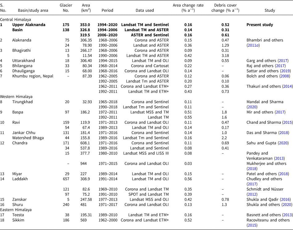
Das and Sharma (Reference Das and Sharma2018) reported the glaciers in Jankar Chhu watershed, Chandrabhaga (Chenab) Basin, had lost area at a rate of 0.16 ± 0.1% a−1 during 1989–2016. The Jankar Chhu watershed has 83 debris-covered glaciers, out of 153 glaciers in the basin. The majority of glaciers (94) are small in size (<0.5 km2). The glaciers of Ravi Basin, Western Himalaya were studied by Chand and Sharma (Reference Chand and Sharma2015) who estimated a loss rate of 0.16 ± 0.4% a−1 during 1989–2010. Patel and others (Reference Patel, Sharma, Fathima and Thamban2018) reported a similar loss rate of 0.16 ± 0.0% a−1 for the Miyar Basin, during 1989–2014. These results are the same as what we observed in the UAB.
However, there are some basins in the western Himalaya, where a higher area loss rate has been reported. For example, Mir and others (Reference Mir, Jain, Jain, Thayyen and Saraf2017) reported a loss rate of 0.51 ± 0.01 a−1 during 1976–2011 in the Baspa Basin. One reason for the higher rates may be due to the use of coarse resolution (60 m) Landsat MSS image; while Mandal and Sharma (Reference Mandal and Sharma2020) observed area loss of 5.6% (0.11% a−1) in the adjacent Tirungkhad watershed, based on relatively high-resolution Corona (1965) and Sentinel (2018) images. Chudley and others (Reference Chudley, Miles and Willis2017) reported a loss of 45.3 km2 (12.8% or 0.52% a−1) in Ladakh range during 1991 and 2014. The difference may be due to exceptionally small size of glaciers and their characteristic (morphology) in this range (Schmidt and Nüsser, Reference Schmidt and Nüsser2012). In the Eastern Himalaya, a loss rate of 0.16 ± 0.3% a−1 was reported in the Tista basin, during 1989–2010 by Basnett and others (Reference Basnett, Kulkarni and Bolch2013).
Overall, given the uncertainties (wherever estimated) in the rate of loss of glacierised area, all the studies seem to indicate that the rate in UAB is roughly the same as that in the rest of Himalaya, namely, ~0.1–0.2% a−1. However, there may be exceptional regions in the western Himalaya where it may be significantly higher.
There were significant changes in the extent of debris cover in the UAB. The rate of change of the fraction of debris cover area in UAB was significantly higher (0.61% a−1) in the period 2006 and 2020 as compared to 0.31% a−1 from 1994 to 2006. The earlier study in UAB observed the similar (0.46% a−1) rate of increase of the debris cover during 1968–2006 (Bhambri and others, Reference Bhambri, Bolch, Chaujar and Kulshreshtha2011a). However, the rate was significantly larger (1.3% a−1) for the period between 1990 and 2006. This may be due to the fact that only 24 glaciers were accounted. Garg and others (Reference Garg, Shukla and Jasrotia2017) report a rate of 0.6% a−1 during 1994–2015 based on 18 glaciers in the Central Himalaya, similar to our results. Overall, the rate of debris-cover increase we report is comparable to the previous studies in the Himalaya (Table 5).
7.4. Regional climatic trends and their impact on glacier change
Climate fluctuations are key to understand glacier variability, the main factors being temperature and precipitation (Oerlemans, Reference Oerlemans2005). While field data close to glaciers are scarce, there are some weather stations in the Himalaya from where data have been reported. To summarise, in the period 1866–2010, an increase in temperature, varying between ~0.1 and ~1°C, and a decrease in precipitation have been reported (Basistha and others, Reference Basistha, Arya and Goel2009; Bhutiyani and others, Reference Bhutiyani, Kale and Pawar2010; Shrestha and Aryal, Reference Shrestha and Aryal2011; Singh and others, Reference Singh, Arya and Chaudhary2013). This is consistent with our analysis of the CRU data plotted in Figure 11. However, we note that after ~2000–2010, the CRU data show a sharp increase in precipitation.
The above discussion motivated us to attempt to interpret the overall changes in the glacier lengths and areas that we observe based on the following regional climate scenario: (a) the regional temperature and precipitation started showing significant positive trends after ~1960–80, (b) the regional temperature increased rapidly in the past three decades or so at a rate of 3–4°C per century, and (c) the regional precipitation decreased from ~1960 to 2010 and then rapidly increased till 2020.
Combining our results with the previous study in UAB by Bhambri and others (Reference Bhambri, Bolch, Chaujar and Kulshreshtha2011a) we conclude that the total glacierised area has decreased from 1968 to 2020 at a constant fractional rate of ~0.015% a–1. This is probably a combined effect of the increase in temperature and decrease in precipitation during this period. Disentangling the two effects requires a basin scale model of the glacier dynamics which we do not attempt. We also observed that average retreat rate of the large UAB glaciers increased from 9.3 ± 1.9 m a−1 (1994–2006) to 13.3 ± 1.8 m a−1 (2006–2020). The length of a glacier responds to temperature changes much quicker than to precipitation changes (Oerlemans, Reference Oerlemans2005). Basically, the temperature changes dominantly affect the ablation zone whereas precipitation changes dominantly affect the accumulation zone. Consequently, it takes time for precipitation changes to reflect in length changes. The response time of length to temperature changes varies from glacier to glacier depending on its size, slope and extent of debris cover (Oerlemans, Reference Oerlemans2005, Banerjee and Shankar, Reference Banerjee and Shankar2013). Our interpretation of the increase in the average retreat rate is that it was dominantly controlled by the warming. The glaciers with larger response times took longer to respond to the changes. Hence, the average retreat rate increased in time and, even though the area and length changes show a delayed response to climate forcing it is evident that the atmospheric warming was the main driver of the glacier wastage in UAB and the whole Himalaya. Long-term high altitude in-situ meteorological records in the basin along with ground-based glaciological measurements (e.g. mass balance, debris thickness) are needed to provide insights on overall glacier response and establish a better relation between glacier changes and climatic parameters.
7.5. Role of glacier-specific factors on area loss
To understand the basin scale area loss, we need to understand the area loss rates of individual glaciers as a function of their attributes since glaciers respond heterogeneously even under similar climatic conditions (Salerno and others, Reference Salerno2017; Brun and others, Reference Brun, Wagnon, Berthier, Jomelli, Maharjan, Shrestha and Kraaijenbrink2019). We have attempted to do this by plotting the relative area loss rates of the glaciers in UAB against several non-climatic attributes (area, debris cover fraction, elevation range and aspect, Fig. 12).

Fig. 12. Scatter plots showing the correlation between area loss (%) during the study period (1994–2020) and non-climatic parameters; (a) glacier area, (b) debris cover %, (c) elevation range, (d) area loss vs aspect.
All the glaciers of UAB show a loss of area between 1994 and 2020. The area loss of individual glaciers ranges from 0.5 to 38%, with a total loss of 4.2 ± 2.9% (0.16 ± 0.11% a−1). This heterogeneous behaviour of glaciers is probably owing to the interplay between topographic and climatic variables. Glacier area loss in UAB is dependent on glacier size and we found a significant negative correlation (r = −0.73) with coefficient of determination (R 2) of 0.53 between area loss (%) and glacier area (size) (Fig. 12a). Similar trends were noticed in the previous studies in Himalaya indicating sensitivity of smaller glaciers to climate change (Kulkarni and others, Reference Kulkarni, Bahuguna, Rathore, Singh, Randhawa, Sood and Dhar2007; Bolch and others, Reference Bolch2012; Chand and Sharma, Reference Chand and Sharma2015). Such small glaciers have short response time and usually adjust their geometry instantly (Huss and Fischer, Reference Huss and Fischer2016). Despite the good correlation between area loss and glacier size in UAB, it is slightly lower than other basins (e.g. Ravi, Miyar, Baspa, Shyok and Jankar) which may be because of relatively higher (1.2 km2) mean glacier size in UAB than these Himalayan basins.
The debris cover of a glacier strongly influences its ablation process. The increasing rate of debris-cover extent over the glaciers is common for shrinking glaciers (Benn and others, Reference Benn2012; Bolch and others, Reference Bolch2012; Kirkbride and Deline, Reference Kirkbride and Deline2013) due to avalanching activity in upper reaches of glacier catchment (Scherler and others, Reference Scherler, Bookhagen and Strecker2011; Laha and others, Reference Laha2017) and the up-glacier shift of SLA (Shukla and Garg, Reference Shukla and Garg2020). The debris-cover area expands up glacier over the time and slowdown the glacier melting (Dobhal and others, Reference Dobhal, Mehta and Srivastava2013; Pratap and others, Reference Pratap, Dobhal, Mehta and Bhambri2015; Shah and others, Reference Shah, Banerjee, Nainwal and Shankar2019), however such glaciers lose mass mainly by thinning not retreat (Banerjee and Shankar, Reference Banerjee and Shankar2013; Ragettli and others, Reference Ragettli, Bolch and Pellicciotti2016; Remya and others, Reference Remya, Kulkarni, Hassan and Nainwal2020). Therefore, we may expect the area loss rate to decrease with increasing fraction of debris cover. A negative correlation (R 2 = 0.15) between glacier area loss and debris-covered fraction was indeed seen (Fig. 12b). Debris-covered glaciers have lost 2.9 ± 2.6% of their area compared to the 10.8 ± 2.8% loss of the debris-free ones. Similar pattern of area loss of debris-covered glaciers was observed in the other Himalayan basin; for example, Sahu and Gupta (Reference Sahu and Gupta2020) reported area loss of ~3% for debris-covered glaciers in comparison with 11% clean ice glaciers in Chanda Basin. Likewise, Mir and others (Reference Mir, Jain, Jain, Thayyen and Saraf2017) observed area change of debris-covered glaciers to be 14% only in Baspa Basin while clean glacier lost an area of 27% during the studied period.
The vertical extent of a glacier is described by its elevation range and mean elevation. The slope of a glacier is derived by dividing the elevation range by its length. Therefore, these two parameters are related to each other. The loss rate is plotted against the elevation range in Figure 12c and good negative correlation (R 2 –0.51) was recorded. Thus, within the uncertainties, the loss rate is inversely proportional to the elevation range. Glaciers with larger elevation ranges will tend to have larger areas and consequently it is not surprising that the loss rate decreases with the increasing elevation range. However, the exponent for the area is ~0.6 whereas for the elevation range it is ~−1. This indicates that the slope plays a significant role in the dynamics.
As expected, the rate of area loss strongly correlates with the aspect as found elsewhere (e.g. DeBeer and Sharp, Reference DeBeer and Sharp2009) (Fig. 12d). The north-south flowing glaciers have been shrinking faster than those flowing east-west. The loss rate of north-facing glaciers was 0.36 ± 0.11% a−1 and it was 0.34 ± 0.11% a−1 for those facing the south. On the contrary, the loss rate of the NW and NE facing glaciers was 0.13 ± 0.11 and 0.15 ± 0.11% a−1 respectively. Similar behaviour has been reported in the previous studies in Alaknanda Basin (Nainwal and others, Reference Nainwal, Negi, Chaudhary, Sajwan and Gaurav2008; Bhambri and others, Reference Bhambri, Bolch, Chaujar and Kulshreshtha2011a). Also, Das and Sharma (Reference Das and Sharma2018) and Sahu and Gupta (Reference Sahu and Gupta2020) found a similar dependence of the area loss on the aspect in Jankar Chhu and Chandra basins, Western Himalaya.
To summarise, the average response of individual glaciers as a function of their non-climatic attributes is typically non-linear. To our knowledge, all past studies (Bhambri and others, Reference Bhambri, Bolch, Chaujar and Kulshreshtha2011a; Chand and Sharma, Reference Chand and Sharma2015; Garg and others, Reference Garg, Shukla and Jasrotia2017; Das and Sharma, Reference Das and Sharma2018; Sahu and Gupta, Reference Sahu and Gupta2020; Shukla and others, Reference Shukla and Garg2020) have analysed this issue using linear regression techniques. Our analysis seems to show that this may not be adequate. We feel that more detailed work needs to be done on this issue.
8. Conclusions
We presented an updated glacier inventory for the UAB for 2020 using Sentinel-2 images and reported the glacier changes in the basin from 1994 to 2020. The updated inventory contains 198 glaciers and shows that the total glacierised area was 354.6 ± 8.5 km2 in 2020.
The glacierised area in the UAB reduced by 15.6 ± 10.6 km2 from 368.6 ± 9.2 km2 in 1994 to 353.0 ± 5.3 km2 in 2020. This implies an average loss rate of 0.16 ± 0.11% a−1 during this period.
Based on the observations of 138 glaciers, a similar rate of area loss was estimated for the time periods, 1994–2006 and 2006–2020 (0.14 ± 0.27 and 0.16 ± 0.19% a−1). According to glacier morphology, the highest area changes were shown by mountain glaciers (10.6%), followed by hanging glaciers (9%) and cirques (8.6%). A significant increase in debris-covered area (13.4 ± 4.4%) was observed during the study period. The retreat of the 20 observed glaciers varied from 4.6 ± 1.8 to 18.9 ± 1.8 m a−1. The average glacier retreat rates increased by ~30% from 9.3 ± 1.9 m a−1 (1994–2006) to 13.3 ± 1.8 m a−1 during the last decade (2006–2020).
The CRU data for the MAT show that warming rates increased to 0.04°C a−1 (for the period 1990–2020) from 0.001°C a−1 (1901–1990) in UAB. Further, a rate of warming of 0.026°C a−1 was observed during 1970–2019. Glacier size, debris-cover extent, elevation range and aspect are found controlling glacier-specific factors for the fractional rate of area loss in UAB from 1994 to 2020. We hope that our data analysis results will motivate modellers to develop physically based models which will eventually result in reliable future projections at a basin scale.
Supplementary material
The supplementary material for this article can be found at https://doi.org/10.1017/jog.2022.87.
Acknowledgements
The field work at Satopanth Glacier was supported by SERB & DST, New Delhi (Grant No. SB/DGH-101/2015 and DST/CCP/NHC/158/2018), IMSc, Chennai and SAC-ISRO funded projects. Parts of the work were conducted in the framework of the project ‘Understanding and quantifying the transient dynamics and evolution of debris-covered glaciers’ funded by the Swiss National Science Foundation (Grant No. 200021-169775). HCN, AM & SS are thankful to the Vice-Chancellor, HNB Garhwal University to provide infrastructural facilities. AM is grateful to Dr Prabhat Semwal for his help in GIS-related issues, and to Dr Argha Banerjee and Dr D. P. Dobhal for their valuable suggestions and discussion during the work. We also acknowledge the USGS (Earth Explorer), European Space Agency (ESA), NASA's Earth Data, and the RGI working group, ICIMOD and A. Sakai (GGI2) for providing satellite images, and other relevant data such as the glacier inventories free of cost. We thank Dr. Rachel Carr, Scientific Editor, and the anonymous reviewers for their valuable comments and suggestions which led to the present improved manuscript.
Author contributions
AM conceptualised the work along with HCN and RS, performed all analysis and wrote the first draft. HCN and RS supervised the research work. T B provided guidance to improve the quality of work. Field work is supported by SSS. All the authors contributed to the final form of the article.
Conflict of interest
None.


 Open access