


1. Introduction
Sea ice is a porous material composed of a multi-phase system of brine, gas, water and ice (Weeks and Ackley, Reference Weeks, Ackley and Untersteiner1982). The structure, composition and texture of sea ice are dependent on its growth conditions. Antarctic sea ice and its field observations are relatively understudied compared to the Arctic. Antarctic sea ice can be found as land-fast ice, drifting pack or consolidated ice, pancake ice, frazil ice and other similar types of sea ice (Weeks, Reference Weeks2010), each with different crystal sizes, structures and stratigraphy's from varying growth conditions. There are two main drivers of sea-ice growth: dynamic and thermodynamic. Dynamic growth by frazil ice accumulation is driven by turbulent ocean conditions that result in accumulation and then consolidation of frazil sea ice. Thermodynamic growth of sea ice results in congelation growth in relatively calm ocean conditions (Weeks, Reference Weeks2010).
There are several distinct textures and shapes of crystals that can be found in sea ice, and each is associated with different growth conditions. Identifying these textures and linking them to certain conditions and activities can assist in helping to understand the complexity of sea-ice growth processes. These textures are polygonal granular, orbicular granular, transitional and columnar (Eicken and Lange, Reference Eicken and Lange1989). Polygonal granular texture is associated with superimposed ice and has large planar crystals. Superimposed ice is formed during the austral spring/summer when the surface snow layer may melt and percolate through a colder snow layer and subsequently refreeze. Orbicular granular texture is marked by smaller and more rounded crystals formed either from the agglomeration of frazil ice (Eicken and Lange, Reference Eicken and Lange1989) or the formation of snow ice (Lytle and Ackley, Reference Lytle and Ackley2001; Arndt and others, Reference Arndt, Haas, Meyer, Peeken and Krumpen2021). Snow ice forms from flooding of the surface snow layer with seawater and its subsequent refreezing (Lange and others, Reference Lange, Schlosser, Ackley, Wadhams and Dieckmann1990; Lytle and Ackley, Reference Lytle and Ackley2001; Arndt and others, Reference Arndt, Haas, Meyer, Peeken and Krumpen2021). Both superimposed ice and snow ice are detected by their negative δ18O values compared to ‘pure’ sea ice (Allison and Worby, Reference Allison and Worby1994), with superimposed ice yielding lower δ18O values compared to snow ice (Arndt and others, Reference Arndt, Haas, Meyer, Peeken and Krumpen2021). Columnar crystal texture is distinct in its long, thin and column-like shape, which is formed in calmer sea states compared to that of orbicular granular crystals. Transitional textures are a combination of these two textures, and thus its defining features are crystals that are beginning to elongate and are in the size range between the granular and columnar textures.
With the combination of low temperatures and turbulent waters, sea ice in the Antarctic marginal ice zone (MIZ) has a great spatial variability throughout the region (Vichi, Reference Vichi2022). Sea-ice growth, especially in the Antarctic, is not commonly found to yield a predictable stratigraphy (Lange and Eicken, Reference Lange and Eicken1991). There have been several reports of sea-ice cores from consolidated pack ice that show rafting or large frazil portions found below columnar structures (Jeffries and Weeks, Reference Jeffries and Weeks1992; Tucker and others, Reference Tucker, Gow, Meese and Bosworth1999; Carnat, and others, Reference Carnat2013; Tison and others, Reference Tison2020). The dynamic nature of the region can lead to deformation-related activities that interrupt the predicted crystal growth of sea ice and its stratigraphy. Four major deformation-related processes have been presented by Lange and Eicken (Reference Lange and Eicken1991) to explain the presence of deformed or unusual crystal stratigraphy. These are (i) ridging and rafting, (ii) rapid formation of frazil from supercooled waters in leads and polynyas, (iii) formation of frazil with regular movement of large floes and (iv) rafting of many floes that leads to gaps and voids between floes. A combination of these four deformation processes is also possible, which can lead to complex core structures.
Most of the textural information on Antarctic sea ice is from pack ice or land-fast ice in summer, and the few data from the MIZ in the other seasons are obtained from the Weddell, Amundsen/Bellingshausen and Ross Sea sectors (Lange and others, Reference Lange, Schlosser, Ackley, Wadhams and Dieckmann1990; Jeffries and others, Reference Jeffries, Li, JañA, Krouse, Hurst-Cushing and Jeffries1998), Reference Jeffries, Krouse, Hurst-Cushing and Maksym2001; Lytle and Ackley, Reference Lytle and Ackley2001; Tison and others, Reference Tison2020) and more recently from Skatulla and others (Reference Skatulla2022) in the eastern Weddell Sea. The MIZ in Antarctica is circumpolar, and much less is known about sea-ice features in other sectors.
Evaluation and understanding of sea-ice morphology in the South Atlantic and Indian regions of the Southern Ocean has historically been lacking, and has been assumed to be similar to the those found in the Weddell Sea or other land-fast sea-ice regions (Clarke and Ackley, Reference Clarke and Ackley1984; Lange and others, Reference Lange, Ackley, Wadhams, Dieckmann and Eicken1989; Lange and Eicken, Reference Lange and Eicken1991; Tison and others, Reference Tison2017). This study presents data from a series of sea-ice stations collected along a transect extending from the 0 to 10°E in Spring 2019. The stations have been selected to highlight the sea-ice stratigraphy and links to deformation processes. This has been supported by an analysis of the back-tracked trajectory of the sampled floes and the associated environmental conditions using earth observation and atmospheric reanalysis products. This study aims to understand and connect the environmental and synoptic conditions of the area to the resulting physical and textural properties of the sea ice.
2. Materials and methods
2.1 Sea-ice stations
The Southern Ocean Seasonal Experiment (SCALE) Spring 2019 Cruise took place from 11 October to 18 November 2019 on board the SA Agulhas II (Ryan-Keogh and Vichi, Reference Ryan-Keogh and Vichi2022). Consolidated sea ice was cored and collected from 24 October to 30 October 2019 at stations SMIZ 2, SMIZ 3, SMIZ 5, SMIZ 6 and SMIZ 7, and brash ice was collected at SMIZ 8 and SMIZ 9, as summarised in Figure 1. The air temperature was measured by the ship's on-board sensors and reported in the dataset provided by Ryan-Keogh (Reference Ryan-Keogh2022). The full sampling protocols followed are described in Skatulla and others (Reference Skatulla2022).
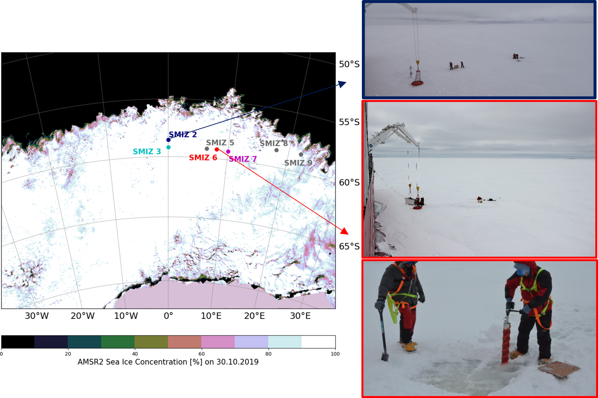
Fig. 1. All sea-ice station locations from the Spring Cruise 2019 shown with the sea-ice concentration from the AMSR2 satellite product on 30 October 2019 (Spreen and others, Reference Spreen, Kaleschke and Heygster2008). Photographs taken by Felix Paul (top), Mike Daniels (middle) and Felix Paul (bottom).
This paper will focus on the results from stations SMIZ 2, SMIZ 3, SMIZ 6 and SMIZ 7, as summarised in Table 1. The more easterly stations, SMIZ 6 and 7, are referred to as the eastern group and SMIZ 2 and 3 are referred to as the western group.
Table 1. Summary of sea ice sampled at consolidated stations in Spring 2019

Core lengths are reported as an average with std dev. from the cores taken for textural analysis and temperature measurement. Air temperature is reported as a daily average of the temperature measured by the onboard Scientific Data Store (Ryan-Keogh, Reference Ryan-Keogh2022). Station conditions are the noteworthy environmental and sea-ice conditions encountered at each station. T + S cores were assigned for temperature and salinity measurement, BGC cores were assigned for δ18O analysis and CS core was used for stratigraphy analysis.
Temperature measurements of sea-ice cores were conducted after extraction from the floe and taken every 5 cm from the bottom of the core to the top. A PT-100 temperature probe, with an accuracy of 0.01°C, was used to measure the temperature once a hole was drilled. This took an average of 6 min to complete for each core. Once the temperature was logged, the core was transported to the mobile polar lab at −10°C where it was segmented using a band saw. The mobile polar lab temperature was chosen to maximise initial processing of samples and a good compromise in which the authors could carry out the work quickly and efficiently. Samples were kept horizontal as much as possible during transport and processing to minimise brine loss. No brine loss from samples was observed (Skatulla and others, Reference Skatulla2022). Each core was cut every 5 cm from the bottom with a band saw and melted in the dark at room temperature in sealed, airtight containers. Each melted sample was then analysed by a 8410A Portasal portable salinometer which has a reported accuracy of <0.003 g kg−1 (OSIL, 2020). A minimum of three cores were collected and analysed per station for temperature and salinity measurements.
The cores destined for texture analysis per station were first prepared using the band saw. The cores were cut into 10 cm segments from the top and subsequently a thick section of 8 mm was cut from the middle of each 10 cm segment. The thermal macrotome is a novel instrument developed for creating 1 mm thin sections with a high temperature nichrome wire. These thin-sections were subsequently viewed through cross-polarised sheets and photographed. This method allows for relatively larger samples than the conventional methods, 10 cm long and 9 cm wide, to be cut for cross-polarisation imaging, without significant sample loss (Johnson, Reference Johnson2020).
Cross-polarisation was performed ~12–24 h after core extraction during the cruise. Using the scale alongside each thin section in an image (see Fig. 4), the size of a crystal can be estimated. From the refraction of light through each crystal, they can be visually distinguished from one another. Each crystal was manually traced and measured. For each image, the average crystal sizes of each ice texture were calculated, using an average of 20 random crystals sized from the images. From visual inspection of the shape of the crystals, in conjunction with their size, the textures found in each sample were identified based on the description and classification by Eicken and Lange (Reference Eicken and Lange1989). From the identified layering of textures in these images, stratigraphy diagrams showing the positions of each texture throughout each core were constructed. The std dev. and 95% confidence interval of the crystal sizes for each identified texture were then calculated for comparison between stations, as described in Skatulla and others (Reference Skatulla2022). After obtaining the cross-polarised images of all the collected cores (see Section 2.1), each set of images was used to construct stratigraphy diagrams to summarise the overall structures and textures of the sea ice.
Oxygen isotope analysis was conducted on samples from SMIZ 6 (δ18O, in ‰ vs. VSMOW = ((18O/16Osample)/(18O/16OVSMOW)–1) × 1000). Three cores were collected, segmented and melted in the dark at room temperature. Meltwater was filtered through a 0.3 μm GF/F filter and subsequently stored in glass exetainers in a fridge. These samples were further filtered through a 0.2 μL filter and analysed using a Picarro Cavity Ring-Down Spectrometer (CRDS) (Walker and others, Reference Walker2016). Oxygen isotope data for stations SMIZ 2, 3 and 7 are not available yet at the time of publication due to logistical reasons.
2.2 Calculation of station ice floe back-track trajectory
To understand the environmental conditions under which the sea ice grew, we estimated the effect of sea-ice drift on the movement of the sea ice through its lifetime. Using the low-resolution sea-ice drift product of the EUMETSAT Ocean and Sea Ice Satellite Application Facility (OSI-SAF) (OSI SAF, 2021) and the OceanParcels Python environment (Delandmeter and van Sebille, Reference Delandmeter and van Sebille2019), the locations of the sampled ice floes were backtracked to its origins in early winter (Fig. 2). The OSI-SAF product consists of daily drift data that are computed over and averaged over 2 days, with each data point covering an area of 62.5 by 62.5 km. This dataset was re-gridded into a 0.5 degrees regular geographic grid with a bilinear interpolation and used in the back-trajectory calculation from the sea ice's growth origin point until the day of sampling.

Fig. 2. Simulated sea-ice station floe trajectories forward in time from the date of sampling to 30 November 2019 shown as the circled points. The smoothed lines are the location of deployed buoys on the respective sea-ice floes on the date of sampling. σ M is the respective mean geodetic distance between the simulated and observed positions.
Trajectories produced with the OSI-SAF data and OceanParcels methodology were verified by simulating the forward trajectories and comparing the resulting trajectories with the tracks of several ice-tethered buoys deployed at the respective stations during the SCALE Spring Cruise 2019 (unpublished data, personal communication from the South African Weather Service). These forward trajectories and the corresponding buoy positions can be seen in Figure 2. The respective mean geodetic distance between the simulated floe positions and the observed buoy locations were calculated and it was found that these distances were within the OSI-SAF grid resolution of 62.5 km, thus validating the use of this method for our analyses.
The divergence of the sea ice along their trajectories was computed using the OSI-SAF drift and velocity datasets on a geographic grid. The divergence field was estimated, averaged over 3 days and smoothed using a low-pass Gaussian filter using the MetPy package (May and others, Reference May2022) in order to associate the broader divergence of the field to that location.
2.3 Sea-ice concentration and atmospheric reanalyses
Data from the Special Sensor Microwave Imager/Sounder (SSMI/S) sea-ice product was obtained which detailed the daily sea-ice concentration of the region from the Defense Meteorological Satellite Program (DMSP) satellites (Maslanik and Stroeve, Reference Maslanik and Stroeve1999). The atmospheric variables were obtained from the ERA5 reanalysis (ECMWF Re-Analysis 5) datasets from 1 June to 1 November 2019 (Hersbach and others, (Reference Hersbach, Bell, Berrisford, Biavati, Horányi, Muñoz Sabater, Nicolas, Peubey, Radu, Rozum, Schepers, Simmons, Soci, Dee and Thépaut2017)). Since the sea-ice drift and concentration products are reported daily, the ERA5 data have been extracted at 12:00 UTC. Vichi and others (Reference Vichi2019) showed that the ERA5 reanalysis dataset is a reliable estimator of the atmospheric state in this sector of the Southern Ocean in winter. Sea-ice concentration and atmospheric variable values (2 m air temperature, sea surface pressure and 10 m wind speed) have been extracted along the trajectory coordinates using a nearest neighbour method.
The distance of each sea-ice floe from the ice edge and the significant wave height at each floe's respective location was estimated using the methods outlined in Womack and others (Reference Womack, Vichi, Alberello and Toffoli2021). In summary, a simple approximation was made whereby the modelled ERA5 wave energy at the sea-ice edge was assumed to travel meridionally south along the same longitude to reach the floe of interest. The wave attenuation coefficient (α) of 6.12 × 10⁻⁶ m−1 used for these calculations was calculated by Womack and others (Reference Womack, Vichi, Alberello and Toffoli2021) under the assumptions of persistent sea-ice type conditions. Attenuation coefficients in the Southern Ocean have been observed to range from 1.6–5.0 × 10⁻⁶ m−1 in low SIC conditions (≤80%) to 26.5–32.7 × 10⁻⁶ m−1 in high SIC (≥80%) in the Ross Sea (Kohout and others, Reference Kohout2020) thus we expect some error in this approximation.
3. Sea-ice properties and crystal structure
3.1 Physical properties
The temperature and salinity profiles of the sea ice collected during the 2019 Spring Cruise can be seen in Figure 3a and Figure 3b respectively. Temperature displayed linear increasing profiles for all cores from stations SMIZ 2 and SMIZ 3 (Fig. 3a), typical of young sea ice (Weeks, Reference Weeks2010). Temperature from SMIZ 6 and SMIZ 7 did not display a clear monotonic downwards profile, but rather the sea ice was warmer and oscillated around a value of −2°C, close to its melting point.
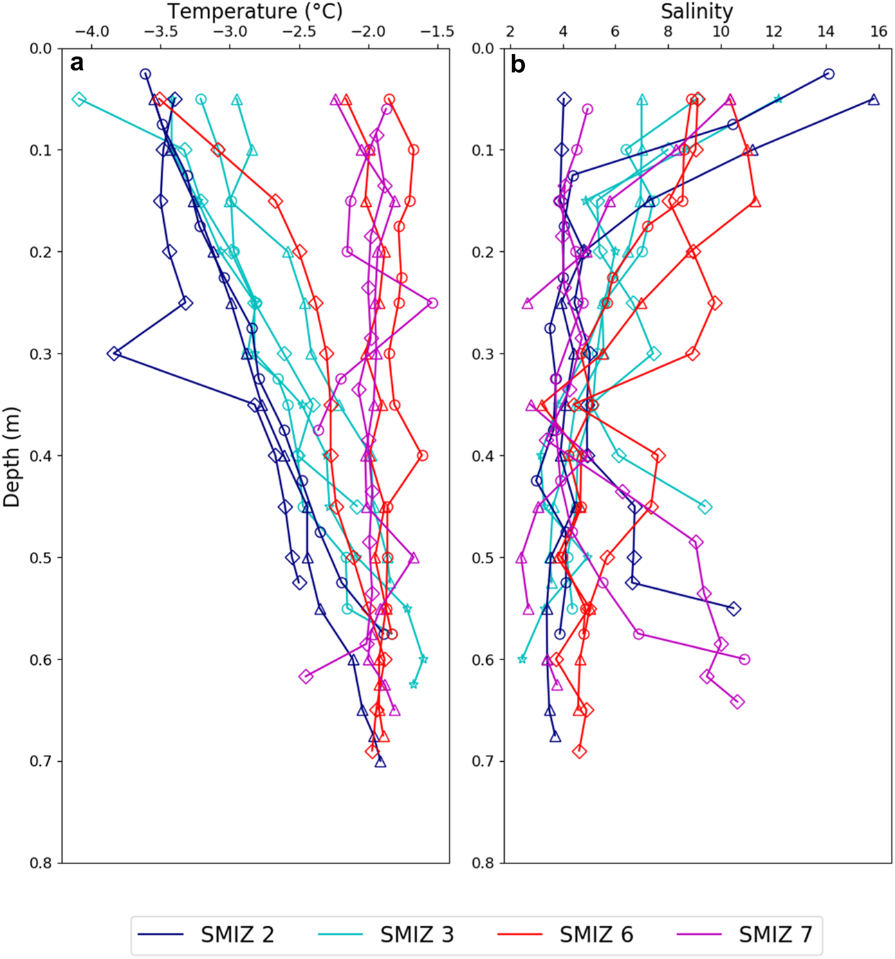
Fig. 3. Physical properties of individual sea-ice cores collected during the SCALE Spring Cruise 2019. (a) Temperature profiles and (b) salinity profiles. Cores collected at each station are distinguished from each other by the different shapes of the markers.
There was a large variability in the salinity profiles from the four sites (Fig. 3b). The cores from SMIZ 2 and SMIZ 3 generally had salinity profiles that resembled a slight C-curve shape, which is a distinguishable feature for first-year sea ice (Weeks and Ackley, Reference Weeks, Ackley and Untersteiner1982; Eicken and Lange, Reference Eicken and Lange1989; Weeks, Reference Weeks2010). Most of these cores had a high surface salinity and a decreasing salinity profile until a slight increase towards the bottom of the sea ice. The sea-ice samples collected from SMIZ 7 exhibited C-curve shapes while having a higher bottom salinity than samples collected from SMIZ 2 and 3. The cores from SMIZ 6 did not display C-shaped profiles. The samples from this station had a higher surface salinity than SMIZ 7, with a decrease with depth. There was not a clear decrease in salinity from the middle to the bottom of the samples, wherein salinity fluctuated between 5 and 8.
The stratigraphy presented in the next section will give further elements to evaluate the difference between the groups of stations.
3.2 Crystal structure and stratigraphy
A summary of the identified textures, and average crystal sizes of each texture in the samples collected at the selected stations, as well as the core lengths can be seen in Table 2. The associated stratigraphy diagrams are seen in Figure 4. We will describe the main features and propose a few hypotheses on their formation, which will be further discussed in Section 5 in conjunction with the reconstructed trajectories.

Fig. 4. Stratigraphy diagrams for sea-ice cores collected at the selected consolidated sea-ice stations with examples of each granular, columnar and transitional textures from SMIZ2, SMIZ 3 and SMIZ 7, respectively.
Table 2. Summary of the frequency of ice textures and statistics found in the collected consolidated sea-ice cores from cross-polarised thin sections

Average crystal sizes are reported with std dev.
Each station had three ice textures: granular, transitional and columnar textures. Distinction between polygonal and orbicular granular textures is difficult when conducting a visual analysis of sea-ice crystals. δ18O analysis is conducted to distinguish between superimposed ice (polygonal granular), snow ice and frazil sea ice (orbicular granular). However, these data are only available for three cores from station SMIZ 6, which will complement the visual interpretation.
The granular texture found in all cores had small crystal sizes (see Table 2), which can be attributed to the fast formation of this ice type in turbulent conditions (Schwerdtfecer, Reference Schwerdtfecer1963). As expected, the transitional textures had larger crystal sizes compared to the granular crystals, and characteristically the columnar ice crystals were significantly larger than any of the other textures.
The stratigraphy of sea ice from SMIZ 2 and SMIZ 3 in Figure 4 both exhibited the typical sea-ice stratigraphy; granular ice found at the surface, followed by transitional and columnar sea ice (Weeks, Reference Weeks2010). The growth conditions for these consolidated sea-ice floes may have been in relatively calm conditions in order for large portions of columnar ice to grow without interruption. These samples had a shorter length and were made up of more than 70% columnar sea-ice texture.
In comparison to the western group of floes SMIZ 2 and 3, the eastern group of SMIZ 6 and 7 both had a higher proportion of granular textures in their respective cores. Due to its complex structure and the availability of the δ18O measurements, we will describe SMIZ 6 in detail in the next section. SMIZ 7's core stratigraphy (Fig. 4) was comprised of mostly granular texture in the upper portion of the core and was subsequently followed by two layers of transitional and columnar ice. The alternating transitional and columnar textures below the granular are indicative of interrupted growth, signalling a dynamic growth environment. SMIZ 7 also had several large air pockets throughout its length, such as that seen in the pink highlighted image in Figure 4.
3.3 Deformation and growth disturbances in SMIZ 6
The sea-ice stratigraphy of the SMIZ 6 core was made up of several unusual layering of textures (Fig. 5). Three cores from this station were analysed for δ18O and their respective profiles can be seen in the graph within Figure 5. These triplicate samples were collected on the same floe and within a few meters of collection of the sample analysed for stratigraphy. The surface of these cores has negative δ18O and increase with depth. One core's negative surface values around −7‰ is indicative of snow ice presence, although the other two cores are slightly below zero at their surface. Beyond the surface granular layer, the δ18O profiles suggest that the granular textures identified deeper in the sea-ice core were formed from frazil sea-ice agglomeration.

Fig. 5. SMIZ 6 core stratigraphy with highlighted segments, a, b and c, shown with cross-polarised images and markers to show noteworthy changes in the sample. The yellow arrow in segment A marks a slanted transition of granular ice into the transitional ice texture beneath the surface. The purple arrow in segment B marks the presence of columnar textures found alongside granular textures. The orange arrow in segment C marks a distinct change from columnar to granular textures. Alongside the core stratigraphy is the δ18O profiles of three samples taken nearby in the field.
There is a slanted transition of granular ice into the transitional ice texture beneath the surface, marked by the yellow arrow in Figure 5. This sloped and irregular transition may have come about from potential rafting of floes. However, we cannot distinguish whether the observed layers were from the rafting activity alone or whether the transitional textures grew in the spaces created after rafting.
Furthermore, below this segment is another indicator of dynamic disturbances in the sea ice's growth. An intrusion of columnar crystals, marked by the purple arrow in Figure 5, is seen alongside granular crystals. A similar combination is seen further down the core with columnar crystals found alongside smaller transitional crystal textures. These points in the core are not indicators of typical sea-ice growth but suppose multiple deformation-related activities that had occurred. It is hypothesised that these adjacent textures could have arisen from the collision of floes comprised of different crystal textures or from the cementing process that forms consolidated pack ice from individual pancake sea-ice floes, as for instance suggested by Lange and Eicken (Reference Lange and Eicken1991).
Below the marked purple segment in Figure 5, there is a clear change in sea-ice texture from columnar to granular crystals shown in orange. This kind of sharp change in textures was seen in similar sea-ice samples upon entering the Terra Nova Bay Polynya in the Ross Sea, presented by Tison and others (Reference Tison2020). They had attributed this feature to rafting activity in the growth process. Rafting is a possible explanation for this feature, however there is no detection of snow ice within the interior of the core, which would indicate the surface of a floe before rafting had occurred (Fig. 5). Rafting, however, may have occurred with little to no snow on the surface of the original floes. An alternative explanation may be the deposition of granular frazil sea ice, which does not have a negative oxygen isotope signature, on the underside of the sea-ice floe as described by Lange and Eicken (Reference Lange and Eicken1991) and hypothesised to be observed in samples by Carnat and others (Reference Carnat2013).
Definitive explanations for the deformation-related activities that may have caused the unusual stratigraphy are difficult to construct and so we can only present the possible and thus probable causes for such complex stratigraphy. Nevertheless, further insight into the growth conditions can be provided by analysing the atmospheric, wave and sea-ice conditions along the backtracked trajectory of the floe throughout its lifetime. This may provide further hints at the drivers that may have led to such complex structures in the SMIZ 6 and SMIZ 7 cores and not in the western SMIZ 2 and SMIZ 3 cores.
4. Sea-ice conditions along the back-trajectories
4.1 Sea-ice floe back-trajectories
Figure 6 shows the estimated trajectory of the floes from the sampling station to the first date when sea-ice drift data are available (Section 2.2). All four sea-ice floes originated to the south-west of their respective sampling points and have moved with the sea-ice drift. Their trajectories show similar features of an initial upward movement of the floes, then a long eastward trajectory. The western group move northward from early October while the eastern group only begin to move slightly northward a few days before sampling took place (see video in Supplementary Information). The sea-ice floes at the stations SMIZ 2, 3, 6 and 7 had similar estimated lifetimes of 141, 140, 140 and 142 days from formation, computed from the first date that OSI-SAF drift data were available until their respective sampling days.
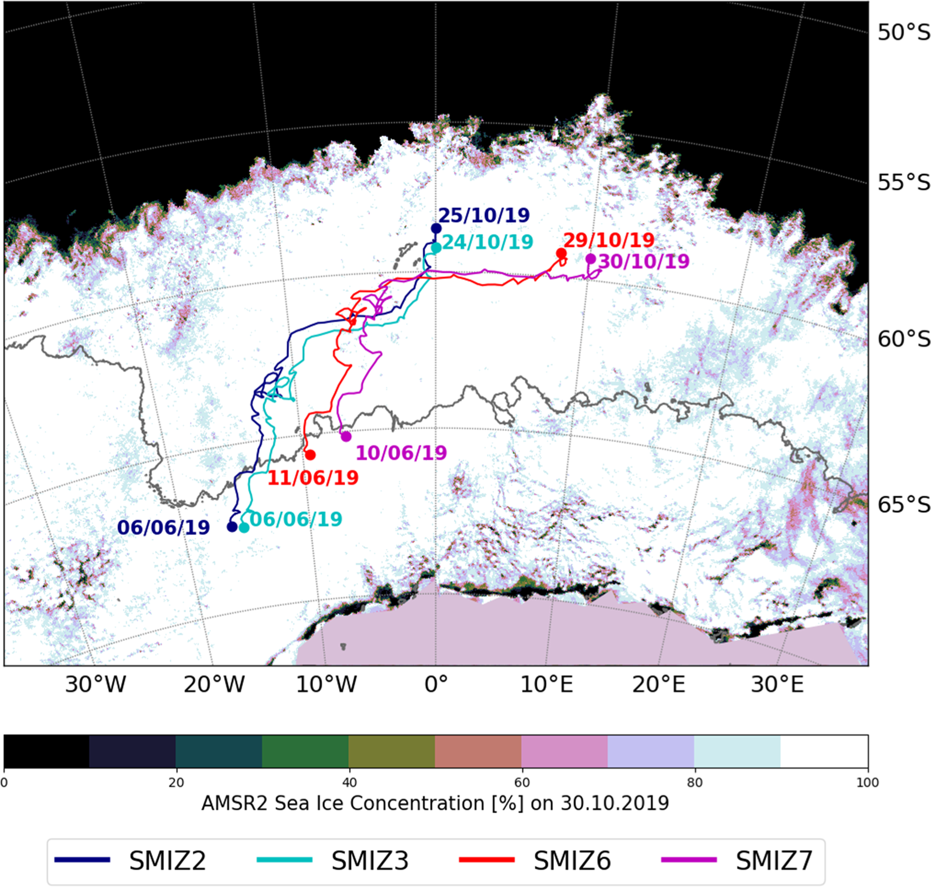
Fig. 6. The reconstructed trajectories of the station's sea-ice floes over the 2019 winter period showing the date and the location of the formation of the ice and the date and location at which the ice floes were sampled (see Table 1). Sea-ice concentration is shown for the last day of sampling, while the grey contour line shows the sea-ice edge on 6 June 2019, the estimated date of formation of the first sea-ice station floe, SMIZ 3. Sea-ice concentration shown is from the AMSR2 product (Spreen and others, Reference Spreen, Kaleschke and Heygster2008).
4.2 Reconstructed history of sea ice and atmospheric conditions
The 2 m air temperature, from ERA5 datasets, along the back-tracked trajectories (Section 2.3) shows the seasonal increase of atmospheric temperatures from July to October (Fig. 7a). The onset of spring can be seen in the overall average increase in atmospheric temperature from September over all station ice floes in Figure 7a. At the time of warming, the floe stations likely underwent a few cases of temperature above −5°C. Fluctuations in temperatures coincided with the passing of low-pressure systems, such as extra-tropical polar cyclones (e.g. Vichi and others, Reference Vichi2019). This is visible in the panels of Figures 7a and b, where most of the temperature increases were found in correspondence with the mean sea level pressure minima. As low-pressure systems passed over the MIZ, warmer oceanic air was pushed over the sea ice, thus resulting in a general opposite fluctuation of temperatures and pressures.
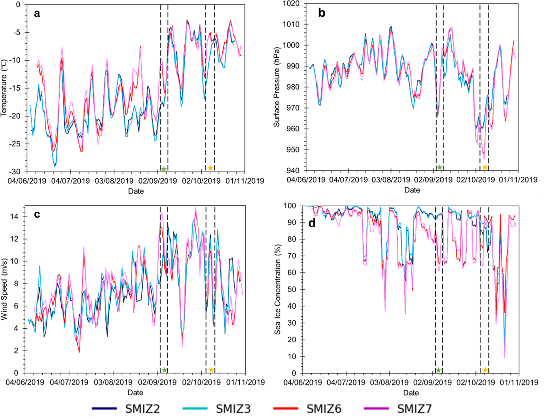
Fig. 7. 2 m temperature (a), surface pressure (b), wind speed (c) and sea-ice concentration (d) averaged over 3 d, extracted along the back-trajectories of the selected sea-ice floes and smoothed with 3 d moving average. All meteorological data have been obtained from the ERA5 product (Section 2.2). Sea-ice concentration values obtained from SSMI/S product. Ticks along the x-axis are 4 d intervals. Dotted black lines highlight the periods of interest where noted storms pass over the region. The green star indicates the period whereby the storm shown in Fig. 8a passes over the region, while the yellow star indicates the period whereby the storm shown in Fig. 8b passes.

Fig. 8. Synoptic map showing the 2 m atmospheric temperature (colour map) and the mean sea level pressure (contours) from ERA5 for the two extra-tropical cyclones over the region of interest on 6 September 2019 (a) and 8 October 2019 (b), with the estimated positions of the sea-ice floes on those dates.
The four stations followed similar temperature fluctuations throughout their respective lifetimes. However, the westward stations, SMIZ 2 and 3, experienced colder temperatures most notably in mid to late August 2019, and floes from SMIZ 6 and 7 deviated from their westward counterparts as they experienced an increase in atmospheric temperature during this period. Additionally, SMIZ 2 and 3 experienced lower temperatures of −17°C in early September and October compared to SMIZ 6 and 7 with temperatures of ~−13°C. Likewise, the floe stations experienced similar conditions associated with the passing of low-pressure systems throughout their lifetimes. This can be seen by the surface pressure at the floe locations in Figure 7b. The significant drop in pressure in early October 2019, marked by the yellow star in Figure 7b, is indicative of a large polar cyclone passing over the region, with pressures as low as 940 hPa. From the surface pressure values, SMIZ 6 and 7 were closer to the core of this polar cyclone.
The wind speed from ERA5 (Section 2.3) extracted over the estimated floe trajectories ranged from 2 to 14 m s−1, as seen in Figure 7c. There was a general increase in wind speed as the floes moved northward into the range of the westerly winds. While the two groups had an overall similar wind speed, there were frequent periods whereby they experienced different wind speeds according to the reanalyses simulation. A major deviation was in late July: SMIZ 2 and 3 experienced a sharp decrease in wind speed from 8 to 3 m s−1, while SMIZ 6 and 7 oscillated around 8 m s−1. In early September, SMIZ 6 and 7 underwent a sudden increase in wind speed from 4 to 14 m s−1. SMIZ 2 and 3 also experienced an increase in wind speed during this period from 5 to 10 m s−1, however it was not as sudden as the eastward group. Despite the differences in wind speeds between the two groups, all floes experienced a sharp decrease in wind speed in mid-September, whereby the wind dropped from ~11 to 2 m s−1, which may have been the result of the passing of a large storm in early September, marked by the green star. Drops in wind speed are often experienced after the passing of a large storm (Alpers and others, Reference Alpers, Liu, Wu, Kirk Cochran, Bokuniewicz and Yager2018).
Sea-ice concentration from the SSMI/S datasets (Section 2.3), as seen in Figure 7d, may give an indication of the state of the sea-ice field and the potential changes that the floes may have undergone during their growth. From Figure 7d, the two groups of floes experienced different changes in sea-ice concentration during their lifetimes. For the initial growth period of June to mid-August 2019, the groups behaved similarly, with common large changes in sea-ice concentration across all floes. From late August onwards to the time of sampling in late October 2019, the two groups deviated from each other. The eastern group of SMIZ 6 and 7 experienced frequent changes from 95% to ~60% concentration throughout this period. However, SMIZ 2 and 3 did not experience such variations in concentration but rather oscillated around a 90–95% sea-ice concentration for the majority of August and September. From mid-October, both groups experienced similar changes in sea-ice concentration again with a sudden decrease in late October before increasing again before sampling began, which may have been the result of the onset of strong southerly winds that pushed the sea ice northward towards open ocean, thus reducing its concentration.
Two large low-pressure systems that passed over the MIZ region in 2019 were identified from the largest drops in surface pressure below 970 hPa from Figure 7b. The passages of the extra-tropical cyclones in Figures 8a and b are marked by the green star and yellow star, respectively, in the panels of Figure 7. The low-pressure system on 8 October 2019 shown in Figure 8b can be classified as an extreme polar cyclone with surface pressures as low as 940 hPa (Wei and Qin, Reference Wei and Qin2016). Changes in atmospheric and sea-ice conditions were found during the passage of these systems with rapid decreases in surface pressure, sea-ice concentration and increases in wind speed (Fig. 7).
The drift divergence experienced by the four floes along their back-trajectories and the overall divergence field over the region were highly variable (Fig. 9 and video in Supplementary Information). As described in Section 2.2, the divergence field was averaged over 3 days and spatially smoothed with a Gaussian filter (Section 2.3), to highlight larger scale effects. The drift data were at an original resolution of 62.5 km; thus divergence or convergence can only be quantitatively inferred on large scales. Negative divergence values indicate a convergence of the field. The divergence of the simulated station floes SMIZ 2 and 3 was very similar throughout their lifetimes, which has been estimated to start from close locations (Fig. 6). The SMIZ 2 and 3 floes had instead opposite divergence conditions at the beginning, likely owing to their larger distance from each other at formation. From the beginning of August 2019, all the floes had a similar divergence field. The most notable difference was found during the polar cyclone in early October (Fig. 8b, marked by the yellow star). The sea-ice field was divergent at the locations of SMIZ 2 and 3 (between −0.02 and −0.04 day1, as observed in the previous events during the year), while SMIZ 6 and 7 experienced a more severe convergence of 0.12 day−1.
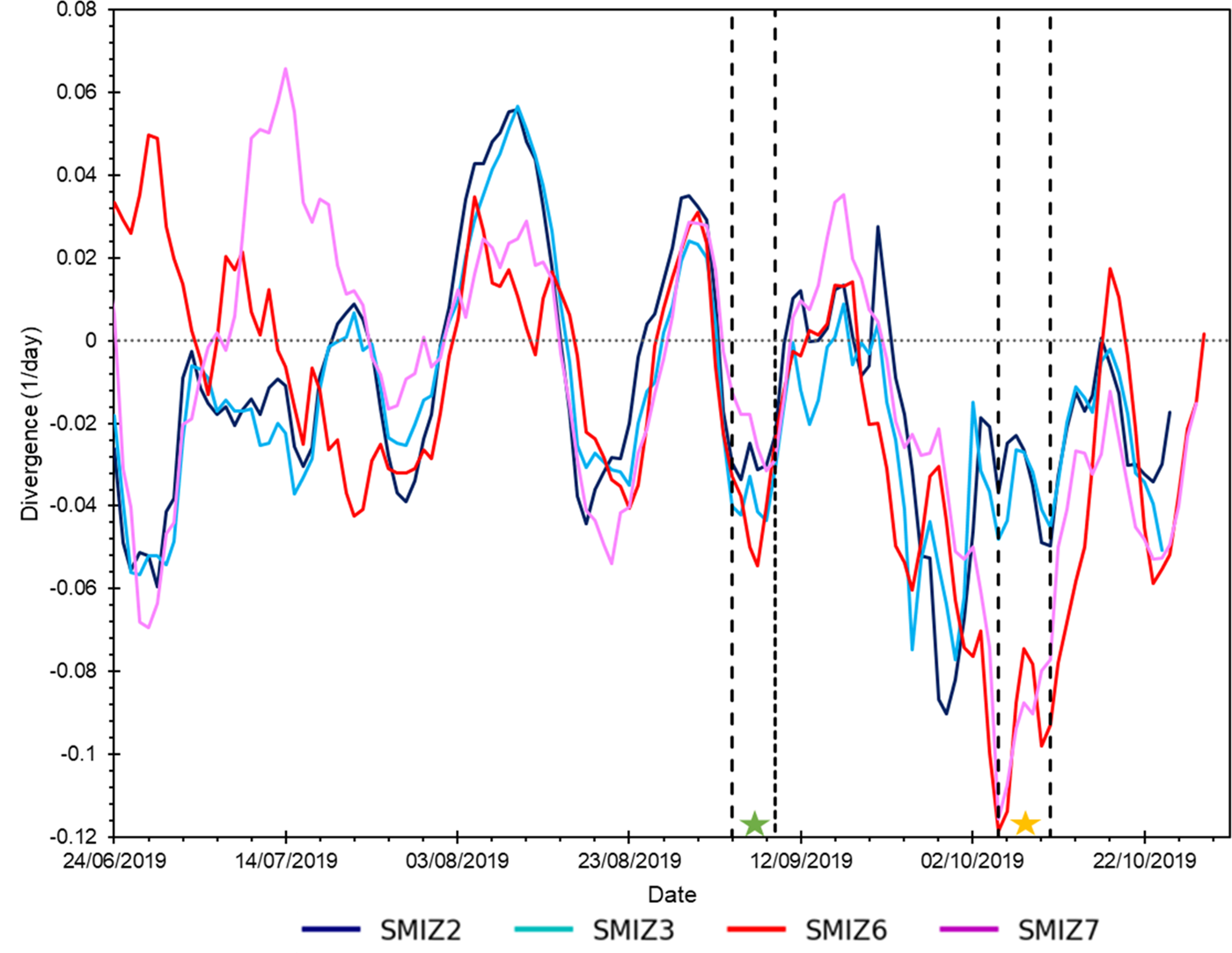
Fig. 9. Sea-ice divergence averaged over 3 d, for the duration of the lifetime of the sea-ice floes collected on the Spring Cruise 2019. Sea-ice divergence obtained from the OSI-SAF sea-ice product and smooth with a low degree Gaussian filter. Ticks along the x-axis are 4 d intervals. Negative divergence values indicate a convergence. Dotted black lines highlight the periods of interest where noted storms pass over the region. The green and yellow stars indicate the period when the cyclones in Fig. 8 passed over the region of interest.
The respective distance from the estimated sea-ice edge to each floe is presented in Figure 10a (Section 2.2). Stations SMIZ 2 and 3 were furthest from the sea-ice edge during the first few months of their lifetimes, compared to SMIZ 6 and 7. There is a significant decrease in distance from the ice edge during late September and early October for SMIZ 2 and 3. This is the same period in which the large polar cyclone in Figure 8b passes over the region. However, SMIZ 6 and 7 did not experience this dramatic decrease in ice edge distance, but their respective distance remained constant from mid-September to mid-October with small fluctuations.

Fig. 10. Distance of floe from the ice edge (a), significant wave height at ice edge (b) and significant wave height at floe position (c) shown for stations SMIZ 2, 3, 6 and 7 and their sea-ice floe's respective position along their back-trajectories. Dotted black lines highlight the periods of interest where noted storms pass over the region. The green star indicates the period whereby the storm shown in Fig. 8a passes over the region, while the yellow star indicates the period whereby the storm shown in Fig. 8b passes.
The significant wave height simulated by ERA5 at the ice edge closest to the station floes (Fig. 10b) showed similar wave activity throughout the lifetime of all station floes. SMIZ 2 and 3 had slightly larger waves than SMIZ 6 and 7. However, under the main assumption of constant wave propagation through sea ice, this difference in the incident wave field was not reflected in the wave height estimated at the locations of the respective floes during the July–September period (Fig. 10c). Floes SMIZ 6 and 7 were estimated to have originated closer to the edge, and thus experienced larger waves over 1.5 m within a month from formation. For the majority of the floe's trajectory, the wave penetration was relatively minimal with significant wave heights below 0.5 m. After the passage of the large polar cyclone in Figure 8b, shown by the green star in Figure 10, the simulated SMIZ 2 and 3 trajectories were closer to the edge, with consequently greater waves from late September until mid-October. SMIZ 6 and 7 also experienced an increase in significant wave height during this time but with a smaller magnitude.
5. Discussion
It is evident from the results shown in the previous section that there was a distinct difference between the two groups of SMIZ 2 and 3 with SMIZ 6 and 7 throughout their respective lifetimes. The synoptic and sea-ice conditions presented suggest that these two groups of floes experienced different conditions in which their distinctly different stratigraphy may have arisen.
5.1 Growth history of the western group
The samples collected at SMIZ 2 and 3 exhibited a documented stratigraphy typical of first-year Antarctic sea ice (Fig. 4) with linear temperature profiles and C-shaped salinity profiles (Fig. 3). Given the observed conditions, it is possible that more than one plausible history could be constructed. Snow depth at the time of collection was above 10 cm, which likely prevented the floe to grow thermodynamically, resulting in a mean core length of <60 cm (see Table 1). However, we speculate that the snow deposition may have been a recent event since the temperature profiles presented in Figure 3a are not homogeneous as would be expected under snow insulation. The triplicate salinity profiles were variable from one another but still exhibited profiles of growing first-year sea ice (Weeks and Ackley, Reference Weeks, Ackley and Untersteiner1982; Eicken and Lange, Reference Eicken and Lange1989; Weeks, Reference Weeks2010; Tison and others, Reference Tison2020). The lack of oxygen isotope data limits our complete characterisation of these floes, although other information supports this conclusion. In addition, the floes that became stations SMIZ 2 and 3 likely had larger wave influence in their initial growth stages (Fig. 10), as well as divergence (Fig. 9). As more sea ice was formed in the area, the stations became more insulated within the sea-ice pack with growing distance from the ice edge (Fig. 10a). During the early months of their growth, the floes at SMIZ 2 and 3 experienced drastic changes in sea-ice concentration alongside their eastern counterparts and corresponding changes in the divergence. With the large decreases in sea-ice concentration in late July and mid-August, there was corresponding convergences in the area. Likewise, the alternating increases to the maximum sea-ice concentration during this period (Fig. 7d) were met with divergences of the sea-ice field (Fig. 9). Despite the variable sea-ice conditions, the interaction of floes within a converging field with low sea-ice concentration or within a diverging field with high sea-ice concentration was likely to yield a low probability of deformation-related activities, such as rafting, which is seen by the lack of disturbance in the samples from SMIZ 2 and 3. We however, cannot confirm that the surface portion is entirely derived from frazil ice agglomeration without the δ18O data at these stations.
After the early growth period, the sea-ice concentrations at the simulated locations of SMIZ 2 and 3 floes reached a maximum in late August (Fig. 7d). A concentration of 90% was maintained for over 2 weeks followed by a decrease after the polar cyclone in early September (Fig. 8a). The sea ice recovered quickly and maintained a near-maximum concentration again for another week. These long stretches of maximum sea-ice concentration likely reduced the wave penetration through the sea-ice pack, as simulated by our simple constant attenuation model. This may have promoted thermodynamic drivers of growth, accounting for the long, uninterrupted columnar portions seen in the SMIZ 2 and 3 samples.
The core lengths of SMIZ 2 and 3 samples were shorter suggesting that growth was interrupted or retracted. Signs of melting within the cores were not evident from the temperature profiles. However, there may have been break-up or reduction of sea ice from the lead-up and duration of the large polar cyclone in early October (Fig. 8b). The passage of the cyclone, with its warmer core temperatures (Vichi and others, Reference Vichi2019), may have induced warming of the floes from the ocean, thus contributing to the reduction in the thickness of these floes. We cannot also exclude the role of waves, which increased after this period when the floes were closer to the edge (Fig. 10c). With relatively more divergence in the area, the stratigraphy of these cores was not interrupted and disturbed in the same way as the eastern group.
5.2 Growth history of the eastern group
The eastern group, SMIZ 6 and 7, are distinct from their western counterparts. The temperature profiles at the time of sampling indicated that the floes were warming with the beginning of the austral spring season (Fig. 3a) and these station sites were reported to have little snow cover (Table 1) which further suggests that the underlying sea ice was not insulated from the atmospheric warming taking place (Fig. 7a) in late October.
The salinity profiles at both sites were a deviation from the typical C-curve shape with high surface and bottom salinities for SMIZ 7 and fluctuating salinities within the middle of the samples for SMIZ 6 (Fig. 3b). Both stations had profiles that may be likened to melting sea ice with a shift maximum salinity downwards (Malmgren, Reference Malmgren and Sverdrup1927; Eicken, Reference Eicken1992). Additionally, SMIZ 6 had salinity profiles that were like those found in a rafted sea-ice sample in the Ross Sea by Tison and others (Reference Tison2020), with fluctuations in the values within the middle of the cores.
SMIZ 7 had an average bottom salinity higher than the other stations, which is also indicative of warming sea ice (Eicken, Reference Eicken1992). This core also had large air pockets throughout its length. It is hypothesised that with an increased temperature shown by Figure 3a, air pockets within the floe may have expanded and connected, such that large, elongated air pockets were clearly observable.
There was a clear and recognisable difference in the stratigraphy of textures between the western and eastern group. The cores collected at SMIZ 6 and 7 suggested a variety of deformation-related activities may have taken place during their lifetime. The large proportion of granular textures in both cores is suggestive of formation in turbulent growth conditions, but with further dynamical reshaping. Our samples were collected in spring, after the whole growing season, and they are characterised by a more complex superposition of layers, which we speculate that it is indicative of deformation-related activities. The negative δ18O in one of the triplicate cores at SMIZ 6 (Fig. 5) indicates the presence of snow ice. Snow ice formation depends on snow depth and ice thickness, and the relative ratio between the two, which determines the buoyancy and eventually a negative freeboard. At the time of sampling, the snow depth was minimal (Table 1), and there was no evidence of flooding prior to sampling. We observed surface melting, as most of the cores from the two sites had homogeneous temperature, and the surface of the ice was characterised by slush (see the site pictures highlighted in red in Fig. 1). It is thus unlikely that two out of the three cores were contaminated by seawater, while one preserved the negative snow-ice signature. Such mixed features are more consistent with possible late-winter flooding, refreezing and dynamical rearrangement, which may have occurred during the passage of the cyclones in September and October.
Given the similarity in the reconstructed trajectories, we expect these features to be present in SMIZ 7; although the granular crystals cannot be distinguished in origin as snow ice or frazil ice, the underlying layering of transitional and columnar textures signalled interrupted growth of the sea ice. The stratigraphy of both cores showed clear signs of growth disruption in multiple places (Fig. 5). The marked changes or the intrusions of different textures within the SMIZ 6 core suggest that frequent deformation-related processes took place along the trajectory of this floe, such as potential collisions, rafting and frazil accumulation on the underside of floes (see Section 3.3) (Lange and Eicken, Reference Lange and Eicken1991).
Our reconstruction indicates that the eastern group experienced different synoptic and sea-ice conditions from SMIZ 2 and 3. Along their respective trajectories, the sea-ice at SMIZ 6 and 7 was exposed to warmer temperatures (Fig. 7a), a greater magnitude of fluctuations in wind speed (Fig. 7c) and seemed to have experienced the polar cyclone in early October more intensely (Figs 7b, 9). These floes were in a more dynamic environment than its western counterparts with greater fluctuations in sea-ice concentrations in the area while SMIZ 2 and 3 maintained stretches of time with near-maximum sea-ice concentration (Fig. 7d).
The incident waves and their height in the interior may also have played a role. The floes that became SMIZ 6 and 7 were closer to the sea-ice edge during the initial growth period (Fig. 10a). However, the wave heights at the floe locations were not considerably different from the other stations (Fig. 10c). This suggests that the variable sea-ice concentration seen at the beginning of winter was not a product of greater wave penetration or proximity to the sea-ice edge. The main difference we can find in the reconstructed history is the role exerted by the passage of two cyclones: the first one in September, which reduced the sea-ice extent and brought the floes closer to the ocean edge (Fig. 10a), and the large polar cyclone in early October (Fig. 4b). Its resultant effects on the sea ice may have contributed to the disruption in the stratigraphy seen in this group of cores. The substantial convergence of the sea-ice field (Fig. 9) together with the increase in wave penetration at SMIZ 6 and 7 in that period (Fig. 10c) could have increased the probability in which deformation-related activities could take place, such as floe collisions and rafting. We acknowledge the limitation of the simple wave attenuation method used in Womack and others (Reference Womack, Vichi, Alberello and Toffoli2021, and Section 4.2). The wave attenuation does not necessarily happen along the shortest pathway to the edge, and it is affected by a range of physical drivers that we are unable to account for (see for instance Montiel and others, Reference Montiel, Kohout and Roach2022). It is an upper-limit diagnostic to combine the distance from the edge with the incident wave sea generated by the passage of the cyclones, and the differences between the reconstructed conditions between the two groups would likely stand with a different attenuation model.
It is also acknowledged that the differences between the groups of stations are based upon the stratigraphy analysis of one sample from a large floe. As a result, variability in structure throughout a floe cannot be accurately represented. This is, however, a difficult issue to address with limited sampling time, challenging and extreme working conditions and expensive analysis techniques. The interpretation of stratigraphy thus cannot be fully dissected and explained. While this is true, we present one of the first datasets of the physical properties of sea ice in this region and have shown marked differences in structure and overall growth conditions between two groups which signal the inherent variability of this region. Despite limited to a few stations, the variability found on this small scale is large, as shown in the temperature, salinity and δ18O data, especially in SMIZ 6.
6. Conclusions
This study presented one of the first datasets on the physical and structural properties of sea ice in the Antarctic MIZ in the Atlantic and Indian sectors of the Southern Ocean, several years after the earlier works by Clarke and Ackley (Reference Clarke and Ackley1984), Jeffries and others (Reference Jeffries, Krouse, Hurst-Cushing and Maksym2001), and complementing the recent data collected in the Ross Sea (Tison and others, Reference Tison2020). The sea ice was collected along the 60°S latitude in late October 2019, starting from the Good Hope Line and moving eastward over a sampling period of 7 days. This study detailed the physical, textural and structural properties of the sea ice and their differences from each other. Upon investigation of the stratigraphy of the sea ice from these stations, it was apparent that the western group of sea-ice cores collected at 0°E (SMIZ 2 and SMIZ 3) has Arctic-like stratigraphy with growth dominated by thermodynamic drivers, while the eastern group (SMIZ 6 and 7) presented disrupted stratigraphy aligned with more dynamic drivers of growth. It is acknowledged that the limited samples presented in this study cannot accurately give an estimate of the variability and inhomogeneity of sea ice in this region and that there may be undetermined variability within a single floe.
The results of this study showcased a sea-ice stratigraphy that is inhomogeneous and complex, which is an indication of a different development of sea-ice structures. The morphology was also different from the sea-ice stratigraphy typically seen in other Antarctic regions such as the Weddell Sea (Lange and others, Reference Lange, Ackley, Wadhams, Dieckmann and Eicken1989) and the Ross Sea (Gow and others, Reference Gow, Ackley, Weeks and Govoni1982, Reference Gow, Ackley, Govoni, Weeks and Jeffries1998; Carnat and others, Reference Carnat2014). These areas can be more conducive to columnar ice in more sheltered sea-ice conditions. Studies conducted in the north-western Weddell Sea (Lange and others, Reference Lange, Schlosser, Ackley, Wadhams and Dieckmann1990; Lange and Eicken, Reference Lange and Eicken1991), and around the Good Hope Line (Clarke and Ackley, Reference Clarke and Ackley1984) also found similar disrupted samples thus indicating that Antarctic sea ice is inhomogeneous, especially in this region. Across these studies, the granular textures made up an average of 64% of samples and were often found in samples that had likely undergone deformation. The total number of samples in this region of the Southern Ocean was however too scarce to warrant an accurate estimation of inhomogeneity, and there has been no investigation until this expedition into the zonal differences along the 60°S latitude in the austral spring. Our findings may help to design the further development of sea-ice numerical models that currently do not include dynamics beyond the elastic, visco-plastic rheology. Other sea-ice characteristics, such as its biogeochemistry, rely on its structure and permeability for favourable exchanges of nutrients and gases within the sea ice. These processes and related properties of sea ice are currently under investigation for the samples collected on the Spring Cruise 2019.
Supplementary material
The supplementary material for this article can be found at https://doi.org/10.1017/jog.2023.21
Data availability
Audh, Riesna R.; Johnson, Siobhan; Hambrock, Mark; Marquart, Rutger; Pead, Justin; Rampai, Tokoloho; Skatulla, Sebastian; Vichi, Marcello. (2022). Sea-ice core temperature and salinity data collected during the 2019 SCALE Spring Cruise (1.0) [Data set]. Zenodo. https://doi.org/10.5281/zenodo.6997631. Johnson, Siobhan; Khoboko, Tsepang; Matlakala, Boitumelo; Vichi, Marcello; Rampai, Tokoloho. (2022). Crystal size and texture data of sea ice from the Antarctic Marginal Ice Zone collected in Spring 2019 [Data set]. Zenodo. https://doi.org/10.5281/zenodo.6966957
Acknowledgements
This work is based on the research supported in part by the National Research Foundation of South Africa (NRF grant No. 118745 and 116801). This work has received funding from the European Union’s Horizon 2020 research and innovation programme under grant agreement no. 101003826 via project CRiceS (Climate Relevant interactions and feedbacks: the key role of sea ice and Snow in the polar and global climate system). We are grateful for the skilled support offered by the captain and crew of the SA Agulhas II during the SCALE Spring expedition. We thank Justin Pead, Mark Hambrock and all the cruise participants who contributed to the success of the sea-ice sampling. Sebastian Skatulla and Keith MacHutchon are acknowledged for supporting the establishment of the UCT mobile polar laboratory. We thank the research office at the University of Cape Town for their financial support. This publication is based on research that has been supported in part by the University of Cape Town's Research Committee (URC).
Author contribution
S. J. wrote the original draft with editing and reviews from T. R. and M. V. S. J. and B. M. performed the cross-polarisation experiments while R. R. A., W. d. J., A. W. and M. V. provided satellite data for analysis. A. W. provided the estimation of the waves in ice, distance of floes from the ice edge and the simulated sea-ice station floe trajectories. S. J., T. R. and M. V. conceptualised this paper and created the methodology followed. R. R. A. provided the unpublished δ18O dataset. M. V. and T. R. provided supervision, funding and resources for the project.
Conflict of interest
None.


 Open access