A Student's Guide to the Schrödinger Equation

Add the x-component of vector \(\vec{A}\) (which is \(3\hat{\imath}\)) to the x-component of vector \(\vec{B}\) (which is \(\hat{\imath}=1\hat{\imath}\)).

Add the y-component of vector \(\vec{A}\) (which is \(-2\hat{\jmath}\)) to the y-component of vector \(\vec{B}\) (which is \(\hat{\jmath}=1\hat{\jmath}\))

The x-component of vector \(\vec{C}=\vec{A}+\vec{B}\) is

\begin{equation*}
C_x=A_x+B_x=3\hat{\imath}+1\hat{\imath}=4\hat{\imath}
\end{equation*}

and the y-component of vector \(\vec{C}=\vec{A}+\vec{B}\) is

\begin{equation*}
C_y=A_y+B_y=-2\hat{\jmath}+1\hat{\jmath}=-1\hat{\jmath}=-\hat{\jmath}
\end{equation*}

so the vector \(\vec{C}\) is

\begin{equation*}
\vec{C}=4\hat{\imath}-\hat{\jmath}.
\end{equation*}

To find the x-component of vector \(\vec{C}\), add the x-component of vector \(\vec{A}\) (which is \(3\hat{\imath}\)) to the x-component of vector \(\vec{B}\) (which is \(\hat{\imath}=1\hat{\imath}\)).

To find the y-component of vector \(\vec{C}\), Add the y-component of vector \(\vec{A}\) (which is \(-2\hat{\jmath}\)) to the y-component of vector \(\vec{B}\) (which is \(\hat{\jmath}=1\hat{\jmath}\)).

This makes the x-component of vector \(\vec{C}=\vec{A}+\vec{B}\)
\begin{equation*}
C_x=A_x+B_x=3\hat{\imath}+1\hat{\imath}=4\hat{\imath}
\end{equation*}
and the y-component of vector \(\vec{C}=\vec{A}+\vec{B}\)\begin{equation*}
C_y=A_y+B_y=-2\hat{\jmath}+1\hat{\jmath}=-1\hat{\jmath}=-\hat{\jmath}
\end{equation*}
so the vector \(\vec{C}\) is
\begin{equation*}
\vec{C}=4\hat{\imath}-\hat{\jmath}.
\end{equation*}

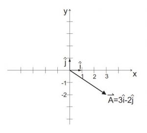
Draw horizontal (x) and vertical (y) axes with unit vector \(\hat{\imath}\) extending one unit along the x-axis and unit vector \(\hat{\jmath}\) extending one unit along the y-axis. Sketch vector \(\vec{A}=3\hat{\imath}-2\hat{\jmath}\) with its base at the origin (\(x=0, y=0)\) and its tip at the point (\(x=3, y=-2)\).

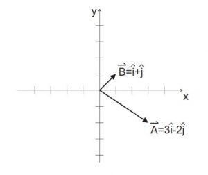
Sketch vector \(\vec{B}=\hat{\imath}+\hat{\jmath}\) with its base at the origin (\(x=0, y=0)\) and its tip at the point (\(x=1, y=1)\).

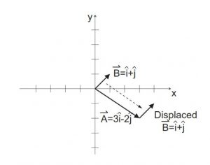
Displace vector \(\vec{B}\) (without changing its length or its direction) so that its base is at the tip of vector \(\vec{A}\).

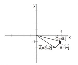
Sketch vector \(\vec{C}\) from the beginning (the base) of vector \(\vec{A}\) to the end (the tip) of vector \(\vec{B}\). Note that vector \(\vec{C}=4\hat{\imath}-\hat{\jmath}\), in agreement with the result of the analytical approach. Note also that you could have achieved the same result by displacing vector \(\vec{A}\) (again without changing its length or its direction) so that its base is at the tip of vector \(\vec{B}\).

Begin by drawing horizontal (x) and vertical (y) axes with unit vector \(\hat{\imath}\) extending one unit along the x-axis and unit vector \(\hat{\jmath}\) extending one unit along the y-axis. Then sketch vector \(\vec{A}=3\hat{\imath}-2\hat{\jmath}\) with its base at the origin (x=0,y=0) and its tip at the point (x=3, y=-2).

Now sketch vector \(\vec{B}=\hat{\imath}+\hat{\jmath}\) with its base at the origin (x=0,y=0) and its tip at the point (x=1,y=1).

The next step is to displace vector \(\vec{B}\) (without changing its length or its direction) so that its base is at the tip of vector \(\vec{A}\).

Finally, sketch vector \(\vec{C}\) from the beginning (the base) of vector \(\vec{A}\) to the end (the tip) of vector \(\vec{B}\). Note that vector \(\vec{C}=4\hat{\imath}-\hat{\jmath}\), in agreement with the result of the analytical approach. Note also that you could have achieved the same result by displacing vector \(\vec{A}\) (again without changing its length or its direction) so that its base is at the tip of vector \(\vec{B}\).

According to Eq. 1.3, the magnitude of vector can be found by squaring and adding the vector’s components and taking the square root of the result.

For the two-dimensional vectors \(\vec{A}\), \(\vec{B}\), and \(\vec{C}\) of Problem 1, the magnitudes can be found using
\begin{align*}
|\vec{A}|&=\sqrt{A_x^2+A_y^2}=\sqrt{(3)^2+(-2)^2}\\
|\vec{B}|&=\sqrt{B_x^2+B_y^2}=\sqrt{(1)^2+(1)^2}\\
|\vec{C}|&=\sqrt{C_x^2+C_y^2}=\sqrt{(4)^2+(1)^2}.
\end{align*}

The values
\begin{align*}
|\vec{A}|&=\sqrt{13}=3.6\\
|\vec{B}|&=\sqrt{2}=1.4\\
|\vec{C}|&=\sqrt{17}=4.1
\end{align*}

can be verified using a ruler to measure the lengths of the vectors in the graph from Problem 1.

According to Eq. 1.3, the magnitude of vector can be found by squaring and adding the vector’s components and taking the square root of the result.

For the two-dimensional vectors \(\vec{A}\), \(\vec{B}\), and \(\vec{C}\) of Problem 1, the magnitudes are
\begin{align*}
|\vec{A}|&=\sqrt{A_x^2+A_y^2}=\sqrt{(3)^2+(-2)^2}=\sqrt{13}=3.6\\
|\vec{B}|&=\sqrt{B_x^2+B_y^2}=\sqrt{(1)^2+(1)^2}=\sqrt{2}=1.4\\
|\vec{C}|&=\sqrt{C_x^2+C_y^2}=\sqrt{(4)^2+(1)^2}=\sqrt{17}=4.1
\end{align*}

as you can verify by measuring the lengths of the vectors in the graph from Problem 1 using a ruler.

Eq. 1.6 tells you that the scalar product between vectors \(\vec{A}\) and \(\vec{B}\) can be found by multiplying the corresponding Cartesian components and summing those products.

For the two-dimensional vectors \(\vec{A}\) and \(\vec{B}\) of Problem 1, the scalar product is
\begin{equation*}
(\vec{A},\vec{B})=\vec{A}\circ\vec{B}=A_xB_x+A_yB_y=(3)(1)+(-2)(1)
\end{equation*}
(remember that these two products are scalars which may be added together to give the scalar value for \(\vec{A}\circ \vec{B}\))

The cosine of the angle between two vectors can be found by dividing the scalar product of the two vectors by the product of the vectors’ magnitudes, as shown in Eq. 1.10.

In this case, the scalar product of the vectors is one and the magnitudes of the two vectors are \(|\vec{A}|=\sqrt{13}\) and \(|\vec{B}|=\sqrt{2}\), so the cosine of the angle between \(\vec{A}\) and \(\vec{B}\) is
\begin{equation*}
\cos{\theta}=\frac{\vec{A}\circ\vec{B}}{|\vec{A}||\vec{B}|}=\frac{1}{\sqrt{13}\sqrt{2}}=\frac{1}{\sqrt{26}}
\end{equation*}
so the angle \(\theta\) may be found by taking the arccosine of this value.

The angle\(\theta=\acos{\frac{1}{\sqrt{26}}}=78.7^\circ\) between vectors\(\vec{A}\) and\(\vec{B}\) may be confirmed using a protractor to find the angle between the vectors on your graph from Problem 1.

Eq. 1.6 tells you that the scalar product between vectors \(\vec{A}\) and \(\vec{B}\) can be found by multiplying the corresponding Cartesian components and summing those products. For the two-dimensional vectors \(\vec{A}\) and \(\vec{B}\) of Problem 1, the scalar product is
\begin{equation*}
(\vec{A},\vec{B})=\vec{A}\circ\vec{B}=A_xB_x+A_yB_y=(3)(1)+(-2)(1)
\end{equation*}
(remember that these two products are scalars which may be added together to give the scalar value for \(\vec{A}\circ \vec{B}\), so the scalar product \(\vec{A}\circ \vec{B}=1\) in this case.)

The cosine of the angle between two vectors can be found by dividing the scalar product of the two vectors by the product of the vectors’ magnitudes, as shown in Eq. 1.10. In this case, the scalar product of the vectors is one and the magnitudes of the two vectors are \(|\vec{A}|=\sqrt{13}\) and \(|\vec{B}|=\sqrt{2}\), so the cosine of the angle between \(\vec{A}\) and \(\vec{B}\) is
\begin{equation*}
\cos{\theta}=\frac{\vec{A}\circ\vec{B}}{|\vec{A}||\vec{B}|}=\frac{1}{\sqrt{13}\sqrt{2}}=\frac{1}{\sqrt{26}}
\end{equation*}
so the angle \(\theta\) may be found by taking the arccosine of this value.

That gives the value of the angle between vectors \(\vec{A}\) and \(\vec{B}\) as $$\theta=acos{\frac{1}{\sqrt{26}}}=78.7^\circ$$ which may be confirmed using a protractor to find the angle between the vectors on your graph from Problem 1.

According to Eq. 1.8, the scalar product between two orthogonal vectors is zero.

As shown in the solution for Problem 3, the dot product between the two-dimensional vectors \(\vec{A}\) and \(\vec{B}\) of Problem 1 is
\begin{equation*}
(\vec{A},\vec{B})=\vec{A}\circ\vec{B}=A_xB_x+A_yB_y=(3)(1)+(-2)(1)=1
\end{equation*}
which means that these two-dimensional vectors are not perpendicular.

To determine whether the three-dimensional vectors \(\vec{A}=3\hat{\imath}-2\hat{\jmath}+\hat{k}\) and \(\vec{B}=\hat{\imath}+\hat{\jmath}-\hat{k}\) are perpendicular, take the scalar product between them to check whether it’s zero.

The scalar product between the 3-D vectors \(\vec{A}\) and \(\vec{B}\) is
\begin{align*}
(\vec{A},\vec{B})&=\vec{A}\circ\vec{B}=A_xB_x+A_yB_y+A_zB_z\\
&=(3)(1)+(-2)(1)+(1)(-1)=0
\end{align*}
so these 3-D vectors are orthogonal.

According to Eq. 1.8, the scalar product between two orthogonal vectors is zero. As shown in the solution for Problem 3, the dot product between the two-dimensional vectors \(\vec{A}\) and \(\vec{B}\) of Problem 1 is
\begin{equation*}
(\vec{A},\vec{B})=\vec{A}\circ\vec{B}=A_xB_x+A_yB_y=(3)(1)+(-2)(1)=1
\end{equation*}
which means that these two-dimensional vectors are not perpendicular.

To determine whether the three-dimensional vectors \(\vec{A}=3\hat{\imath}-2\hat{\jmath}+\hat{k}\) and \(\vec{B}=\hat{\imath}+\hat{\jmath}-\hat{k}\) are perpendicular, take the scalar product between them to check whether it’s zero. The scalar product between the 3-D vectors \(\vec{A}\) and \(\vec{B}\) is
\begin{align*}
(\vec{A},\vec{B})&=\vec{A}\circ\vec{B}=A_xB_x+A_yB_y+A_zB_z\\
&=(3)(1)+(-2)(1)+(1)(-1)=0
\end{align*}
so these 3-D vectors are orthogonal.

As described in Section 1.2, the square of the norm of ket \(\ket{A}\) can be found by operating on ket \(\ket{A}\) with bra \(\bra{A}\).

For ket
\begin{equation*}
\ket{\psi}=4\ket{\epsilon_1}-2i\ket{\epsilon_2}+i\ket{\epsilon_3}=\begin{pmatrix}4\\-2i\\i \end{pmatrix}
\end{equation*}
the corresponding bra is
\begin{equation*}
\bra{\psi}=\left(4^*\; -2i^*\; i^*\right)=(4\; 2i\; -i).
\end{equation*}

The inner product of \(\psi\) with itself is
\begin{align*}
\braket{\psi\vert\psi}&=(4\; 2i\; -i)\begin{pmatrix}4\\-2i\\i \end{pmatrix}=(4)(4)+(2i)(-2i)+(-i)(i)\\
&=16+4+1.
\end{align*}

Since \(|\psi|^2=\braket{\psi\vert\psi}=21\), the norm of \(\psi\) is
\begin{equation*}
|\psi|=\sqrt{21}.
\end{equation*}

Dividing ket \(\ket{\psi}\) by its norm gives the normalized version of \(\ket{\psi}\):
\begin{equation*}
\ket{\psi}=\frac{1}{\sqrt{21}}\left(4\ket{\epsilon_1}-2i\ket{\epsilon_2}+i\ket{\epsilon_3}\right)=\frac{1}{\sqrt{21}}\begin{pmatrix}4\\-2i\\i \end{pmatrix}.
\end{equation*}

As described in Section 1.2, the square of the norm of ket \(\ket{A}\) can be found by operating on ket \(\ket{A}\) with bra \(\bra{A}\). For ket
\begin{equation*}
\ket{\psi}=4\ket{\epsilon_1}-2i\ket{\epsilon_2}+i\ket{\epsilon_3}=\begin{pmatrix}4\\-2i\\i \end{pmatrix}
\end{equation*}
the corresponding bra is
\begin{equation*}
\bra{\psi}=\left(4^*\; -2i^*\; i^*\right)=(4\; 2i\; -i).
\end{equation*}

The inner product of \(\psi\) with itself is therefore
\begin{align*}
\braket{\psi\vert\psi}&=(4\; 2i\; -i)\begin{pmatrix}4\\-2i\\i \end{pmatrix}=(4)(4)+(2i)(-2i)+(-i)(i)\\
&=16+4+1,
\end{align*}

and since \(|\psi|^2=\braket{\psi\vert\psi}=21\), the norm of \(\psi\) is
\begin{equation*}
|\psi|=\sqrt{21}.
\end{equation*}

Dividing ket \(\ket{\psi}\) by its norm gives the normalized version of \(\ket{\psi}\):
\begin{equation*}
\ket{\psi}=\frac{1}{\sqrt{21}}\left(4\ket{\epsilon_1}-2i\ket{\epsilon_2}+i\ket{\epsilon_3}\right)=\frac{1}{\sqrt{21}}\begin{pmatrix}4\\-2i\\i \end{pmatrix}.
\end{equation*}

To form the inner product \(\braket{\phi\vert\psi}\), start by finding the bra \(\bra{\phi}\) that is the dual of ket \(\ket{\phi}\).

The bra \(\bra{\phi}\) that is the dual of ket \(\ket{\phi}=3i\ket{\epsilon_1}+\ket{\epsilon_2}-5i\ket{\epsilon_3}\) is
\begin{equation*}
\bra{\phi}=(3i^*\; 1^*\; -5i^*)=(-3i\; 1\; 5i).
\end{equation*}

Forming the inner product using the bra \(\bra{\phi}\) from the previous hint and ket \(\ket{\psi}\) gives
\begin{align*}
\braket{\phi\vert\psi}&=(-3i\; 1\; 5i)\begin{pmatrix}4\\-2i\\i \end{pmatrix}\\
&=(-3i)(4)+(1)(-2i)+(5i)(i).
\end{align*}

To show that \(\braket{\phi\vert\psi}=\braket{\psi}{\phi}^*\), find the bra \(\bra{\psi}\) that is the dual of ket \(\ket{\psi}\) and multiply that bra by the ket \(\ket{\phi}\).

The bra \(\bra{\psi}\) that is the dual of ket \(\ket{\psi}\) is
\begin{equation*}
\bra{\psi}=(4^*\; -2i^*\; i^*)=(4\; 2i\; -i).
\end{equation*}

Multiplying bra \(\bra{\psi}\) by ket \(\ket{\phi}\) gives
\begin{align*}
\braket{\psi\vert\phi}&=(4\; 2i\; -i)\begin{pmatrix}3i\\1\\-5i \end{pmatrix}\\
&=12i+2i-5.
\end{align*}

To form the inner product \(\braket{\phi\vert\psi}\), start by finding the bra \(\bra{\phi}\) that is the dual of ket \(\ket{\phi}\). This bra is
\begin{equation*}
\bra{\phi}=(3i^*\; 1^*\; -5i^*)=(-3i\; 1\; 5i),
\end{equation*}
and forming the inner product of this bra with ket \(\ket{\psi}\) gives
\begin{align*}
\braket{\phi\vert\psi}&=(-3i\; 1\; 5i)\begin{pmatrix}4\\-2i\\i \end{pmatrix}\\
&=(-3i)(4)+(1)(-2i)+(5i)(i)=-14i-5.
\end{align*}

To show that \(\braket{\phi\vert\psi}=\braket{\psi\vert\phi}^*\), find the bra \(\bra{\psi}\) that is the dual of ket \(\ket{\psi}\) and multiply that bra by the ket \(\ket{\phi}\). This bra is
\begin{equation*}
\bra{\psi}=(4^*\; -2i^*\; i^*)=(4\; 2i\; -i),
\end{equation*}

and multiplying this bra by ket \(\ket{\phi}\) gives
\begin{align*}
\braket{\psi\vert\phi}&=(4\; 2i\; -i)\begin{pmatrix}3i\\1\\-5i \end{pmatrix}\\
&=12i+2i-5=14i-5.
\end{align*}

Comparing the inner-product result for \(\braket{\phi\vert\psi}\) with the result for \(\braket{\psi\vert\phi}\) shows
\begin{align*}
\braket{\phi\vert\psi}&=-14i-5\\
\braket{\psi\vert\phi}&=14i-5
\end{align*}
so \(\braket{\phi\vert\psi}=\braket{\psi\vert\phi}^*\).

As described in Section 1.5, two functions are orthogonal if the inner product between the functions equals zero:
\begin{equation*}
(f(x),g(x))=\braket{f(x)\vert g(x)}=\int_{-\infty}^{\infty}f^*(x)g(x)dx=0.
\end{equation*}

If you make the function \(f(x)=\sin{mx}\) and the function \(g(x)=\sin{nx}\), the inner product is
\begin{equation*}
(f(x),g(x))=\int_{0}^{2\pi}(\sin{mx})^*(\sin{nx})\:dx.
\end{equation*}

Since \((\sin{mx})^*=\sin{mx}\), you can use the integral relation
\begin{equation*}
\int\sin{mx}\sin{nx}\;dx=\left[\frac{\sin{(m-n)}x}{2(m-n)}+\frac{\sin{(m+n)}x}{2(m+n)}\right]
\end{equation*}
in which \(m\) and \(n\) are different integers.

Using the integral relation from the previous hint gives
\begin{align*}
\int_0^{2\pi}\sin{mx}\sin{nx}\;dx&=\left[\frac{\sin{(m-n)}x}{2(m-n)}+\frac{\sin{(m+n)}x}{2(m+n)}\right]\Bigr|_{0}^{2\pi}\\
&=\left[\frac{\sin{(m-n)}2\pi}{2(m-n)}+\frac{\sin{(m+n)}2\pi}{2(m+n)}\right]\\
&\hspace{1cm}-\left[\frac{\sin{(m-n)}0}{2(m-n)}+\frac{\sin{(m+n)}0}{2(m+n)}\right].
\end{align*}

Since \(m\) and \(n\) are different integers, the difference \(m-n\) and the sum \(m+n\) are also an integers, and the sine of any integer multiple of \(2\pi\) is zero. The sine of zero is also zero.

For the interval \(x=0\) to \(x=\frac{3\pi}{2}\), use the same process with these limits on the integrals:
\begin{align*}
\int_0^{\frac{3\pi}{2}}\sin{mx}\sin{nx}\;dx&=\left[\frac{\sin{(m-n)}x}{2(m-n)}+\frac{\sin{(m+n)}x}{2(m+n)}\right]\Bigr|_{0}^{\frac{3\pi}{2}}\\
&=\left[\frac{\sin{(m-n)}\frac{3\pi}{2}}{2(m-n)}+\frac{\sin{(m+n)}\frac{3\pi}{2}}{2(m+n)}\right]\\
&\hspace{1cm}-\left[\frac{\sin{(m-n)}0}{2(m-n)}+\frac{\sin{(m+n)}0}{2(m+n)}\right].
\end{align*}

The term \(\frac{\sin{(m-n)}\frac{3\pi}{2}}{2(m-n)}\) and the term
\(\frac{\sin{(m+n)}\frac{3\pi}{2}}{2(m+n)}\) can take on various values, depending on the values of \(m\) and \(n\), but the difference between these two terms is not, in general, equal to zero (specifically, when \(m-n\) is odd).

As described in Section 1.5, two functions are orthogonal if the inner product between the function equals zero:
\begin{equation*}
(f(x),g(x))=\braket{f(x)\vert g(x)}=\int_{-\infty}^{\infty}f^*(x)g(x)dx=0.
\end{equation*}

If you make the function \(f(x)=\sin{mx}\) and the function \(g(x)=\sin{nx}\), the inner product is
\begin{equation*}
(f(x),g(x))=\int_{0}^{2\pi}(\sin{mx})^*(\sin{nx})\:dx.
\end{equation*}

Since \((\sin{mx})^*=\sin{mx}\), you can use the integral relation
\begin{equation*}
\int\sin{mx}\sin{nx}\;dx=\left[\frac{\sin{(m-n)}x}{2(m-n)}+\frac{\sin{(m+n)}x}{2(m+n)}\right]
\end{equation*}
in which \(m\) and \(n\) are different integers.

Using this integral relation gives
\begin{align*}
\int_0^{2\pi}\sin{mx}\sin{nx}\;dx&=\left[\frac{\sin{(m-n)}x}{2(m-n)}+\frac{\sin{(m+n)}x}{2(m+n)}\right]\Bigr|_{0}^{2\pi}\\
&=\left[\frac{\sin{(m-n)}2\pi}{2(m-n)}+\frac{\sin{(m+n)}2\pi}{2(m+n)}\right]\\
&\hspace{1cm}-\left[\frac{\sin{(m-n)}0}{2(m-n)}+\frac{\sin{(m+n)}0}{2(m+n)}\right].
\end{align*}

Since \(m\) and \(n\) are different integers, the difference \(m-n\) is also an integer, and the sine of any integer multiple of \(2\pi\) is zero. The sine of zero is also zero, so
\begin{equation*}
(f(x),g(x))=\int_{0}^{2\pi}(\sin{mx})^*(\sin{nx})\:dx=0
\end{equation*}

and these two functions are orthogonal over the interval of 0 to \(2\pi\).

For the interval \(x=0\) to \(x=\frac{3\pi}{2}\), use the same process with these limits on the integrals:
\begin{align*}
\int_0^{\frac{3\pi}{2}}\sin{mx}\sin{nx}\;dx&=\left[\frac{\sin{(m-n)}x}{2(m-n)}+\frac{\sin{(m+n)}x}{2(m+n)}\right]\Bigr|_{0}^{\frac{3\pi}{2}}\\
&=\left[\frac{\sin{(m-n)}\frac{3\pi}{2}}{2(m-n)}+\frac{\sin{(m+n)}\frac{3\pi}{2}}{2(m+n)}\right]\\
&\hspace{1cm}-\left[\frac{\sin{(m-n)}0}{2(m-n)}+\frac{\sin{(m+n)}0}{2(m+n)}\right].
\end{align*}

The term \(\frac{\sin{(m-n)}\frac{3\pi}{2}}{2(m-n)}\) and the term
\(\frac{\sin{(m+n)}\frac{3\pi}{2}}{2(m+n)}\) can take on various values, depending on the values of \(m\) and \(n\), but the difference between these two terms is not, in general, equal to zero (specifically, when \(m-n\) is odd). Hence these two functions are not orthogonal over the interval of 0 to \(3\pi/2\) if \(m-n\) is odd.

To serve as an orthonormal basis over the specified interval, these functions must be orthogonal over this interval and must have unity norm.

To determine if these two functions are orthogonal over the interval \(t=0\) to \(t=T\), evaluate the integral
\begin{equation*}
\int_0^Te^{-i\omega t}e^{2i\omega t}dt
\end{equation*}
with \(\omega=\frac{2\pi}{T}\).

To evaluate the integral given in the previous hint, combine the two terms by adding their exponents and integrating:
\begin{equation*}
\int_0^Te^{-i\omega t}e^{2i\omega t}dt=\int_0^T e^{i\omega t}dt=\frac{1}{i\omega}e^{i\omega t}\Bigr|_0^T.
\end{equation*}

Since
\begin{equation*}
\frac{1}{i\omega}\left(e^{i\omega T}-e^{i\omega 0}\right)=\frac{1}{i\omega}\left(e^{i\frac{2\pi}{T} T}-e^{i\frac{2\pi}{T} 0}\right)=\frac{1}{i\omega}\left(e^{i(2\pi)}-e^0\right),
\end{equation*}

and\(e^{i(2\pi)}=\cos{2\pi}+i\sin{2\pi}=1\), the integral
\begin{equation*}
\int_0^T e^{-i\omega t}e^{2i\omega t}dt=\frac{1}{i\omega}(1-1)=0.
\end{equation*}

To determine if the functions \(e^{i\omega t}\) and\(e^{2i\omega t}\) have unity norm, use Eq. 1.27:
\begin{equation*}
|{f(x)}|=\sqrt{\braket{f(x)|f(x)}}=\sqrt{\int_{-\infty}^{\infty}f^*(x)f(x)dx}
\end{equation*}

which in this case is
\begin{equation*}
|{e^{-i\omega t}}|=\sqrt{\int_{0}^{T}e^{+i\omega t}e^{-i \omega t}dt}
\end{equation*}

and

\begin{equation*}
|{e^{2i\omega t}}|=\sqrt{\int_{0}^{T}e^{-2i\omega t}e^{2i \omega t}dt}.
\end{equation*}

The integrals of the previous hint evaluate to
\begin{equation*}
|{e^{-i\omega t}}|=\sqrt{\int_{0}^{T}e^{0}dt}=\sqrt{T}
\end{equation*}

and

\begin{equation*}
|{e^{2i\omega t}}|=\sqrt{\int_{0}^{T}e^{0}dt}=\sqrt{T}
\end{equation*}

so these functions do not have unity norm, but they can be normalized by dividing each by\(\sqrt{T}\).

To serve as an orthonormal basis over the specified interval, these functions must be orthogonal over this interval and must have unity norm. To determine if these two functions are orthogonal over the interval \(t=0\) to \(t=T\), evaluate the integral
\begin{equation*}
\int_0^Te^{-i\omega t}e^{2i\omega t}dt
\end{equation*}
with \(\omega=\frac{2\pi}{T}\).

To evaluate this integral, combine the two terms by adding their exponents and integrating:
\begin{equation*}
\int_0^Te^{-i\omega t}e^{2i\omega t}dt=\int_0^T e^{i\omega t}dt=\frac{1}{i\omega}e^{i\omega t}\Bigr|_0^T.
\end{equation*}

And since
\begin{equation*}
\frac{1}{i\omega}\left(e^{i\omega T}-e^{i\omega 0}\right)=\frac{1}{i\omega}\left(e^{i\frac{2\pi}{T} T}-e^{i\frac{2\pi}{T} 0}\right)=\frac{1}{i\omega}\left(e^{i(2\pi)}-e^0\right),
\end{equation*}

and \(e^{i(2\pi)}=\cos{2\pi}+i\sin{2\pi}=1\), the integral
\begin{equation*}
\int_0^T e^{-i\omega t}e^{2i\omega t}dt=\frac{1}{i\omega}(1-1)=0,
\end{equation*}
so these two functions are orthogonal to one another.

To determine if the functions \(e^{i\omega t}\) and \(e^{2i\omega t}\) have unity norm, use Eq. 1.27:
\begin{equation*}
|{f(x)}|=\sqrt{\braket{f(x)|f(x)}}=\sqrt{\int_{-\infty}^{\infty}f^*(x)f(x)dx}
\end{equation*}

which in this case is
\begin{equation*}
|{e^{-i\omega t}}|=\sqrt{\int_{0}^{T}e^{+i\omega t}e^{-i \omega t}dt}
\end{equation*}
and
\begin{equation*}
|{e^{2i\omega t}}|=\sqrt{\int_{0}^{T}e^{-2i\omega t}e^{2i \omega t}dt}.
\end{equation*}

These integrals evaluate to
\begin{equation*}
|{e^{-i\omega t}}|=\sqrt{\int_{0}^{T}e^{0}dt}=\sqrt{T}
\end{equation*}
and
\begin{equation*}
|{e^{2i\omega t}}|=\sqrt{\int_{0}^{T}e^{0}dt}=\sqrt{T},
\end{equation*}
so these functions do not have unity norm, but they can be normalized by dividing each by\(\sqrt{T}\).

You can find the components of a vector in the direction of each basis vector by taking the inner product between the vector and each basis vector, as shown in Eq. 1.32.

In this case, inserting the basis vector \(\vec{\epsilon}_1\) and vector \(\vec{A}\) into Eq. 1.32 gives
\begin{equation*}
A_1=\frac{\vec{\epsilon}_1 \circ \vec{A}}{\vert\vec{\epsilon}_1\vert^2}=\frac{3\hat{\imath} \circ (6\hat{\imath}+6\hat{\jmath}+6\hat{k})}{\vert3\hat{\imath}\vert^2}.
\end{equation*}

Since \(\hat{\imath}\circ \hat{\imath}=1\) and \(\hat{\imath}\circ \hat{\jmath}=\hat{\imath} \circ \hat{k}=0\), the expression in the previous hint is
\begin{equation*}
A_1=\frac{3\hat{\imath} \circ (6\hat{\imath}+6\hat{\jmath}+6\hat{k})}{\vert3\hat{\imath}\vert^2}=\frac{(3)(6)(1)+(3)(6)(0)+(3)(6)(0)}{(3^2)+(0^2)+(0^2)}
\end{equation*}

The same process using basis vector \(\vec{\epsilon}_2\) and vector \(\vec{A}\) gives
\begin{equation*}
A_2=\frac{(4\hat{\jmath}+4\hat{k}) \circ (6\hat{\imath}+6\hat{\jmath}+6\hat{k})}{\vert4\hat{\jmath}+4\hat{k}\vert^2}=\frac{(4)(6)(1)+(4)(6)(1)}{(4^2)+(4^2)}
\end{equation*}

and using basis vector \(\vec{\epsilon}_3\) and vector \(\vec{A}\) gives
\begin{equation*}
A_3=\frac{(-2\hat{\jmath}+\hat{k}) \circ (6\hat{\imath}+6\hat{\jmath}+6\hat{k})}{\vert-2\hat{\jmath}+\hat{k}\vert^2}=\frac{(-2)(6)(1)+(1)(6)(1)}{(-2^2)+(1^2)}.
\end{equation*}

You can find the components of a vector in the direction of each basis vector by taking the inner product between the vector and each basis vector, as shown in Eq. 1.32. In this case, inserting the basis vector \(\vec{\epsilon}_1\) and vector \(\vec{A}\) into Eq. 1.32 gives
\begin{equation*}
A_1=\frac{\vec{\epsilon}_1 \circ \vec{A}}{\vert\vec{\epsilon}_1\vert^2}=\frac{3\hat{\imath} \circ (6\hat{\imath}+6\hat{\jmath}+6\hat{k})}{\vert3\hat{\imath}\vert^2},
\end{equation*}

and since \(\hat{\imath}\circ \hat{\imath}=1\) and \(\hat{\imath}\circ \hat{\jmath}=\hat{\imath} \circ \hat{k}=0\), this expression is
\begin{align*}
A_1=\frac{3\hat{\imath} \circ (6\hat{\imath}+6\hat{\jmath}+6\hat{k})}{\vert3\hat{\imath}\vert^2}&=\frac{(3)(6)(1)+(3)(6)(0)+(3)(6)(0)}{(3^2)+(0^2)+(0^2)}\\
&=\frac{18}{9}=2.
\end{align*}
The same process using basis vector \(\vec{\epsilon}_2\) and vector \(\vec{A}\) gives
\begin{align*}
A_2=\frac{(4\hat{\jmath}+4\hat{k}) \circ (6\hat{\imath}+6\hat{\jmath}+6\hat{k})}{\vert4\hat{\jmath}+4\hat{k}\vert^2}&=\frac{(4)(6)(1)+(4)(6)(1)}{(4^2)+(4^2)}\\
&=\frac{48}{32}=1.5
\end{align*}

and using basis vector \(\vec{\epsilon}_3\) and vector \(\vec{A}\) gives
\begin{align*}
A_3=\frac{(-2\hat{\jmath}+\hat{k}) \circ (6\hat{\imath}+6\hat{\jmath}+6\hat{k})}{\vert-2\hat{\jmath}+\hat{k}\vert^2}=&\frac{(-2)(6)(1)+(1)(6)(1)}{(-2^2)+(1^2)}\\
&=\frac{-6}{5}=-1.2.
\end{align*}

To determine values of \(c_1\), \(c_2\), \(c_3\), and \(c_4\) (the “amount” of each basis function \(\psi_1(x)\), \(\psi_2(x)\), \(\psi_3(x)\), and \(\psi_4(x)\) contained in function \(f(x)\)), use Eq. 1.36:
\begin{align*}
c_1&=\frac{\braket{\psi_1\vert\psi}}{\braket{\psi_1\vert\psi_1}}=\frac{\int_{-\infty}^{\infty}\psi_1^*(x)\psi(x)dx}{\int_{-\infty}^{\infty}\psi_1^*(x)\psi_1(x)dx}\\
c_2&=\frac{\braket{\psi_2\vert\psi}}{\braket{\psi_2\vert\psi_2}}=\frac{\int_{-\infty}^{\infty}\psi_2^*(x)\psi(x)dx}{\int_{-\infty}^{\infty}\psi_2^*(x)\psi_2(x)dx}\\
c_N&=\frac{\braket{\psi_N\vert\psi}}{\braket{\psi_N\vert\psi_N}}=\frac{\int_{-\infty}^{\infty}\psi_N^*(x)\psi(x)dx}{\int_{-\infty}^{\infty}\psi_N^*(x)\psi_N(x)dx}
\end{align*}

with \(\psi(x)=f(x)=1\) between \(x=0\) and \(x=L\).

For \(c_1\), the “amount” of \(\psi_1=\sin{(\frac{\pi x}{L})}\) contained in the function \(f(x)=1\) between \(x=0\) and \(x=L\), the first portion of Eq. 1.36 looks like this:
\begin{align*}
c_1&=\frac{\int_{-\infty}^{\infty}\psi_1^*(x)\psi(x)dx}{\int_{-\infty}^{\infty}\psi_1^*(x)\psi_1(x)dx}\\
&=\frac{\int_{0}^{L}\left[\sin{(\frac{\pi x}{L})}\right]^*\left[1\right]dx}{\int_{0}^{L}\left[\sin{(\frac{\pi x}{L})}\right]^*\left[\sin{(\frac{\pi x}{L})}\right]dx}.
\end{align*}

The integrals in the previous hint can be evaluated using
\begin{equation*}
\int_{0}^{L}\left[\sin{\left(\frac{\pi x}{L}\right)}\right]dx=
\left[-\cos{\left(\frac{\pi x}{L}\right)}\right]\left[\frac{L}{\pi}\right]\Bigr|_0^L
\end{equation*}

and
\begin{equation*}
\int_{0}^{L}\left[\sin{(\frac{\pi x}{L})}\right]^2dx=\left[\frac{x}{2}-\frac{\sin{\left(\frac{2\pi x}{L}\right)}}{4\left(\frac{\pi}{L}\right)}\right]\Bigr|_0^L.
\end{equation*}

Plugging in the limits gives
\begin{align*}
\int_{0}^{L}\left[\sin{\left(\frac{\pi x}{L}\right)}\right]dx&=
\left[-\cos{\left(\frac{\pi L}{L}\right)}\right]\left[\frac{L}{\pi}\right]-\left[-\cos{\left(\frac{\pi (0)}{L}\right)}\right]\left[\frac{L}{\pi}\right]\\
&=-(-1)\frac{L}{\pi}+\frac{L}{\pi}=\frac{2L}{\pi}
\end{align*}

and
\begin{align*}
\int_{0}^{L}\left[\sin{(\frac{\pi x}{L})}\right]^2dx&=\left[\frac{L}{2}-\frac{\sin{\left(\frac{2\pi L}{L}\right)}}{4\left(\frac{\pi}{L}\right)}\right]-\left[\frac{0}{2}-\frac{\sin{\left(\frac{2\pi (0)}{L}\right)}}{4\left(\frac{\pi}{L}\right)}\right]\\
&=\frac{L}{2}.
\end{align*}

Thus
\begin{equation*}
c_1=\frac{\frac{2L}{\pi}}{\frac{L}{2}}=\frac{4}{\pi}.
\end{equation*}

Using the same approach gives \(c_2\):
\begin{align*}
c_2&=\frac{\int_{-\infty}^{\infty}\psi_2^*(x)\psi(x)dx}{\int_{-\infty}^{\infty}\psi_1^*(x)\psi_2(x)dx}\\
&=\frac{\int_{0}^{L}\left[\cos{(\frac{\pi x}{L})}\right]^*\left[1\right]dx}{\int_{0}^{L}\left[\cos{(\frac{\pi x}{L})}\right]^*\left[\cos{(\frac{\pi x}{L})}\right]dx}.
\end{align*}

which can be evaluated using
\begin{equation*}
\int_{0}^{L}\left[\cos{\left(\frac{\pi x}{L}\right)}\right]dx=
\left[\sin{\left(\frac{\pi x}{L}\right)}\right]\left[\frac{L}{\pi}\right]\Bigr|_0^L=0
\end{equation*}

and

\begin{equation*}
\int_{0}^{L}\left[\cos{(\frac{\pi x}{L})}\right]^2dx=\left[\frac{x}{2}-\frac{\sin{\left(\frac{2\pi x}{L}\right)}}{4\left(\frac{\pi}{L}\right)}\right]\Bigr|_0^L=\frac{L}{2}.
\end{equation*}

Thus \(c_2=\frac{0}{\frac{L}{2}}=0\).

Using the same approach gives \(c_3\):
\begin{align*}
c_3&=\frac{\int_{-\infty}^{\infty}\psi_3^*(x)\psi(x)dx}{\int_{-\infty}^{\infty}\psi_3^*(x)\psi_1(x)dx}\\
&=\frac{\int_{0}^{L}\left[\sin{(\frac{2\pi x}{L})}\right]^*\left[1\right]dx}{\int_{0}^{L}\left[\sin{(\frac{2\pi x}{L})}\right]^*\left[\sin{(\frac{2\pi x}{L})}\right]dx}.
\end{align*}

which can be evaluated using
\begin{align*}
\int_{0}^{L}\left[\sin{\left(\frac{2\pi x}{L}\right)}\right]dx&=
\left[-\cos{\left(\frac{2\pi x}{L}\right)}\right]\left[\frac{L}{2\pi}\right]\Bigr|_0^L\\
&=\left[-1\right]\left[\frac{L}{2\pi}\right]-\left[-1\right]\left[\frac{L}{2\pi}\right]=0
\end{align*}

and

\begin{equation*}
\int_{0}^{L}\left[\sin{(\frac{2\pi x}{L})}\right]^2dx=\left[\frac{x}{2}-\frac{\sin{\left(\frac{4\pi x}{L}\right)}}{8\left(\frac{\pi}{L}\right)}\right]\Bigr|_0^L=\frac{L}{2}.
\end{equation*}

Thus \(c_3=\frac{0}{\frac{L}{2}}=0\).

Using the same approach gives \(c_4\):
\begin{align*}
c_4&=\frac{\int_{-\infty}^{\infty}\psi_4^*(x)\psi(x)dx}{\int_{-\infty}^{\infty}\psi_1^*(x)\psi_4(x)dx}\\
&=\frac{\int_{0}^{L}\left[\cos{(\frac{2\pi x}{L})}\right]^*\left[1\right]dx}{\int_{0}^{L}\left[\cos{(\frac{2\pi x}{L})}\right]^*\left[\cos{(\frac{2\pi x}{L})}\right]dx}.
\end{align*}

which can be evaluated using
\begin{equation*}
\int_{0}^{L}\left[\cos{\left(\frac{2\pi x}{L}\right)}\right]dx=
\left[\sin{\left(\frac{2\pi x}{L}\right)}\right]\left[\frac{L}{2\pi}\right]\Bigr|_0^L=0
\end{equation*}

and

\begin{equation*}
\int_{0}^{L}\left[\cos{(\frac{2\pi x}{L})}\right]^2dx=\left[\frac{x}{2}-\frac{\sin{\left(\frac{4\pi x}{L}\right)}}{8\left(\frac{\pi}{L}\right)}\right]\Bigr|_0^L=\frac{L}{2}.
\end{equation*}

Thus \(c_4=\frac{0}{\frac{L}{2}}=0\).

To determine values of \(c_1\), \(c_2\), \(c_3\), and \(c_4\) (the “amount” of each basis function \(\psi_1(x)\), \(\psi_2(x)\), \(\psi_3(x)\), and \(\psi_4(x)\) contained in function \(f(x)\)), use Eq. 1.36:
\begin{align*}
c_1&=\frac{\braket{\psi_1\vert\psi}}{\braket{\psi_1\vert\psi_1}}=\frac{\int_{-\infty}^{\infty}\psi_1^*(x)\psi(x)dx}{\int_{-\infty}^{\infty}\psi_1^*(x)\psi_1(x)dx}\\
c_2&=\frac{\braket{\psi_2\vert\psi}}{\braket{\psi_2\vert\psi_2}}=\frac{\int_{-\infty}^{\infty}\psi_2^*(x)\psi(x)dx}{\int_{-\infty}^{\infty}\psi_2^*(x)\psi_2(x)dx}\\
c_N&=\frac{\braket{\psi_N\vert\psi}}{\braket{\psi_N\vert\psi_N}}=\frac{\int_{-\infty}^{\infty}\psi_N^*(x)\psi(x)dx}{\int_{-\infty}^{\infty}\psi_N^*(x)\psi_N(x)dx}
\end{align*}

with \(\psi(x)=f(x)=1\) between \(x=0\) and \(x=L\).

For \(c_1\), the “amount” of \(\psi_1=\sin{(\frac{\pi x}{L})}\) contained in the function \(f(x)=1\) between \(x=0\) and \(x=L\), the first portion of Eq. 1.36 looks like this:
\begin{align*}
c_1&=\frac{\int_{-\infty}^{\infty}\psi_1^*(x)\psi(x)dx}{\int_{-\infty}^{\infty}\psi_1^*(x)\psi_1(x)dx}\\
&=\frac{\int_{0}^{L}\left[\sin{(\frac{\pi x}{L})}\right]^*\left[1\right]dx}{\int_{0}^{L}\left[\sin{(\frac{\pi x}{L})}\right]^*\left[\sin{(\frac{\pi x}{L})}\right]dx}.
\end{align*}

These integrals can be evaluated using
\begin{equation*}
\int_{0}^{L}\left[\sin{\left(\frac{\pi x}{L}\right)}\right]dx=
\left[-\cos{\left(\frac{\pi x}{L}\right)}\right]\left[\frac{L}{\pi}\right]\Bigr|_0^L
\end{equation*}

and
\begin{equation*}
\int_{0}^{L}\left[\sin{(\frac{\pi x}{L})}\right]^2dx=\left[\frac{x}{2}-\frac{\sin{\left(\frac{2\pi x}{L}\right)}}{4\left(\frac{\pi}{L}\right)}\right]\Bigr|_0^L
\end{equation*}

and plugging in the limits gives
\begin{align*}
\int_{0}^{L}\left[\sin{\left(\frac{\pi x}{L}\right)}\right]dx&=
\left[-\cos{\left(\frac{\pi L}{L}\right)}\right]\left[\frac{L}{\pi}\right]-\left[-\cos{\left(\frac{\pi (0)}{L}\right)}\right]\left[\frac{L}{\pi}\right]\\
&=-(-1)\frac{L}{\pi}+\frac{L}{\pi}=\frac{2L}{\pi}
\end{align*}

and
\begin{align*}
\int_{0}^{L}\left[\sin{(\frac{\pi x}{L})}\right]^2dx&=\left[\frac{L}{2}-\frac{\sin{\left(\frac{2\pi L}{L}\right)}}{4\left(\frac{\pi}{L}\right)}\right]-\left[\frac{0}{2}-\frac{\sin{\left(\frac{2\pi (0)}{L}\right)}}{4\left(\frac{\pi}{L}\right)}\right]\\
&=\frac{L}{2}.
\end{align*}

Thus
\begin{equation*}
c_1=\frac{\frac{2L}{\pi}}{\frac{L}{2}}=\frac{4}{\pi}.
\end{equation*}

Using the same approach gives \(c_2\):
\begin{align*}
c_2&=\frac{\int_{-\infty}^{\infty}\psi_2^*(x)\psi(x)dx}{\int_{-\infty}^{\infty}\psi_1^*(x)\psi_2(x)dx}\\
&=\frac{\int_{0}^{L}\left[\cos{(\frac{\pi x}{L})}\right]^*\left[1\right]dx}{\int_{0}^{L}\left[\cos{(\frac{\pi x}{L})}\right]^*\left[\cos{(\frac{\pi x}{L})}\right]dx}.
\end{align*}

which can be evaluated using
\begin{equation*}
\int_{0}^{L}\left[\cos{\left(\frac{\pi x}{L}\right)}\right]dx=
\left[\sin{\left(\frac{\pi x}{L}\right)}\right]\left[\frac{L}{\pi}\right]\Bigr|_0^L=0
\end{equation*}

and

\begin{equation*}
\int_{0}^{L}\left[\cos{(\frac{\pi x}{L})}\right]^2dx=\left[\frac{x}{2}-\frac{\sin{\left(\frac{2\pi x}{L}\right)}}{4\left(\frac{\pi}{L}\right)}\right]\Bigr|_0^L=\frac{L}{2}.
\end{equation*}

Thus \(c_2=\frac{0}{\frac{L}{2}}=0\).

Using the same approach gives \(c_3\):
\begin{align*}
c_3&=\frac{\int_{-\infty}^{\infty}\psi_3^*(x)\psi(x)dx}{\int_{-\infty}^{\infty}\psi_3^*(x)\psi_1(x)dx}\\
&=\frac{\int_{0}^{L}\left[\sin{(\frac{2\pi x}{L})}\right]^*\left[1\right]dx}{\int_{0}^{L}\left[\sin{(\frac{2\pi x}{L})}\right]^*\left[\sin{(\frac{2\pi x}{L})}\right]dx}.
\end{align*}

which can be evaluated using
\begin{align*}
\int_{0}^{L}\left[\sin{\left(\frac{2\pi x}{L}\right)}\right]dx&=
\left[-\cos{\left(\frac{2\pi x}{L}\right)}\right]\left[\frac{L}{2\pi}\right]\Bigr|_0^L\\
&=\left[-1\right]\left[\frac{L}{2\pi}\right]-\left[-1\right]\left[\frac{L}{2\pi}\right]=0
\end{align*}

and

\begin{equation*}
\int_{0}^{L}\left[\sin{(\frac{2\pi x}{L})}\right]^2dx=\left[\frac{x}{2}-\frac{\sin{\left(\frac{4\pi x}{L}\right)}}{8\left(\frac{\pi}{L}\right)}\right]\Bigr|_0^L=\frac{L}{2}.
\end{equation*}

Thus \(c_3=\frac{0}{\frac{L}{2}}=0\).\\

Using the same approach gives \(c_4\):
\begin{align*}
c_4&=\frac{\int_{-\infty}^{\infty}\psi_4^*(x)\psi(x)dx}{\int_{-\infty}^{\infty}\psi_1^*(x)\psi_4(x)dx}\\
&=\frac{\int_{0}^{L}\left[\cos{(\frac{2\pi x}{L})}\right]^*\left[1\right]dx}{\int_{0}^{L}\left[\cos{(\frac{2\pi x}{L})}\right]^*\left[\cos{(\frac{2\pi x}{L})}\right]dx}.
\end{align*}

which can be evaluated using
\begin{equation*}
\int_{0}^{L}\left[\cos{\left(\frac{2\pi x}{L}\right)}\right]dx=
\left[\sin{\left(\frac{2\pi x}{L}\right)}\right]\left[\frac{L}{2\pi}\right]\Bigr|_0^L=0
\end{equation*}

and

\begin{equation*}
\int_{0}^{L}\left[\cos{(\frac{2\pi x}{L})}\right]^2dx=\left[\frac{x}{2}-\frac{\sin{\left(\frac{4\pi x}{L}\right)}}{8\left(\frac{\pi}{L}\right)}\right]\Bigr|_0^L=\frac{L}{2}.
\end{equation*}

Thus \(c_4=\frac{0}{\frac{L}{2}}=0\).