
Introduction
Nonmonotonic logic (abbreviated as NML) and its domain, defeasible reasoning, are multifaceted areas. In crafting an Element that serves as both an introduction and an overview, we must adopt a specific perspective to ensure coherence and systematic coverage. It is, however, in the nature of illuminating a scenario with a spotlight that certain aspects emerge prominently, while others recede into shadow. The focus of this Element is on unveiling the core ideas and concepts underlying NML. Rather than exhaustively presenting concrete logics from existing literature, we emphasize three fundamental methods: (i) formal argumentation, (ii) consistent accumulation, and (iii) semantic approaches.
An argumentative approach for understanding human reasoning has been proposed both in a philosophical context by Toulmin’s forceful attack on formal logic in Reference Toulmin1958, and more recently in cognitive science by Mercier and Sperber (Reference Mercier and Sperber2011). Pioneers such as Pollock (Reference Pollock1991) and Dung (Reference Dung1995) have provided the foundation for a rich family of systems of formal argumentation.
Consistent accumulation methods are based on the idea that an agent facing possibly conflicting and not fully reliable information is well advised to reason on the basis of only a consistent part of that information. The agent could start with certain information and then stepwise add merely plausible information. In this way they stepwise accumulate a consistent foundation to reason with. Accumulation methods cover, for instance, Reiter’s influential default logic (Reiter, Reference Reiter1980) or methods based on maximal consistent sets, such as early logics by Rescher and Manor (Reference Rescher and Manor1970) and (constrained) input–output logic (Makinson & Van Der Torre, Reference Makinson and Van Der Torre2001).
While the previous two methods are largely based on syntactic or proof-theoretic considerations, interpretation plays the essential role in semantic approaches. The core idea is to order interpretations with respect to normality considerations and then to select sufficiently normal ones. These are used to determine the consequences of a reasoning process or to give meaning to nonmonotonic conditionals. The idea surfaces in the history of NML in many places, among others in Batens (Reference Batens1986), Gelfond and Lifschitz (Reference Gelfond and Lifschitz1988), Kraus et al. (Reference Kraus, Lehman and Magidor1990), McCarthy (Reference McCarthy1980), and Shoham (Reference Shoham and Ginsberg1987).
A central aspect of this Element is its unifying perspective (inspired by works such as Bochman (Reference Bochman2005) and Makinson (Reference Makinson2005). Defeasible reasoning gives rise to a variety of formal models based on different assumptions and approaches. Comparing these approaches can be difficult. The Element presents several translations between NMLs, illustrating that in many cases the same inferences can be validated in terms of diverse formal methods. These translations offer numerous benefits. They enrich our understanding by offering different perspectives: the same underlying inference mechanism may be considered as a form of (formal) argumentation, a way of reasoning with interpretations that are ordered with respect to their plausibility, or as a way of accumulating and reasoning with consistent subsets of a possibly inconsistent knowledge base. They demonstrate the robustness of the underlying inference mechanism, since several intuitive methods give rise to the same result. While the different methodological strands of NML have often been developed with little cross-fertilization, it is remarkable that the resulting systems can often be related with relative ease. Finally, the translations may convince the reader that, despite the fact that the field of NML seems a bit of a rag rug at first sight, there is quite some coherence when taking a deeper dive. In particular, by showcasing formal argumentation’s exceptional ability to represent other NMLs, this Element adds further evidence to the fruitfulness of Dung’s program of utilizing formal argumentation as a unifying perspective on defeasible reasoning (Dung, Reference Dung1995).
The Element is organized in four parts. Part I provides a general introduction to the topic of defeasible reasoning and NML. The three core methods are each introduced in a nutshell. It provides a condensed and self-contained overview of the fundamentals of NML for readers with limited time. Part II to IV deepen on each of the respective methods by providing metatheoretic insights and presenting concrete systems from the literature.
While some short metaproofs that contribute to an improved understanding are left in the body of the Element, two technical appendices are provided for others. In particular, results marked with ‘⋆’ are proven in the appendices.
Many important aspects and systems of NML didn’t get the spotlight and fell victim to the trade-off between systematicity and scope from which an introductory Element of this length will necessarily suffer. Nevertheless, with this Element a reader will grow the wings necessary to maneuver in the lands of nonflying birds, that is, they will be well equipped to understand, say, first-order versions of logics that are discussed here on the propositional level, or systems such as autoepistemic logic.
Part I Logics for Defeasible Reasoning
1 Defeasible Reasoning
1.1 What is Defeasible Reasoning?
We certainly want more than we can get by deduction from our evidence. … So real inference, the inference we need for the conduct of life, must be nonmonotonic.
This Element introduces logical models of defeasible reasoning, so-called NonMonotonic Logics (in short, NMLs). When we reason, we make inferences, that is, we draw conclusions from some given information or basic assumptions. Whenever we reserve the possibility to retract some inferences upon acquiring more information, we reason defeasibly.Footnote 1 Two paradigmatic examples of defeasible inferences are:
| Assumption | Defeasible conclusion | Reason for retraction |
| The streets are wet. | It rained. | The streets have been cleaned. |
| Tweety is a bird. | Tweety can fly. | Tweety is a penguin. |
As the examples highlight, we often reason defeasibly if our available information is incomplete: we lack knowledge of what happened before we observed the wet streets, or we lack knowledge of what kind of bird Tweety is. Defeasible inferences often add new information to our assumptions: while being explanatory of the streets being wet, the fact that it rained is not contained in the fact that the streets are wet, and while being able to fly is a typical property of birds, being a bird does not necessitate being able to fly. In this sense defeasible inferences are ampliative.
Logics that may lose conclusions once more information is acquired are called nonmonotonic. The vast majority of logics the reader will typically encounter in logic textbooks are monotonic, with classical logic (in short, CL) being the celebrity. Whenever the given assumptions are true, an inference sanctioned by CL will securely pass the torch from the assumptions to the conclusion, warranting with absolute certainty the truth of the conclusion. Truth is preserved in inferences sanctioned by CL. No matter how much information we add, how many inferences we chain between our premises and our final conclusion, or how often the torch is passed, truth endures: the flames reach their final destination. Thus, inferences are never retracted in CL, and conclusions accumulate the more assumptions we add. This property, called monotonicity, is highly desirable for certain domains of reasoning such as mathematics, a domain where CL reigns.
However, a key motivation behind the development of NML is that out in the wild of commonsense, expert, or scientific reasoning, good inferences need not be truth preservational: we often change our minds and retract inferences when watching a crime show and wondering who the most likely murderer is; medical doctors may change their diagnosis with the arrival of more evidence, and so do scientists, sometimes resulting in scientific revolutions. In less idealized circumstances than those of purely formal sciences (such as mathematics), we usually need to reason with incomplete, sometimes even conflicting information. As a consequence, our inferences allow for exceptions and/or criticism. They are adaptable: learning or inferring more information may cause retraction, previous inferences may get defeated. Outside the ivory tower of mathematics, in the stormy domain of commonsense reasoning, the torch’s fire may get extinguished.
It is therefore not surprising that examples of defeasible reasoning are abundant. In what follows, we will list some paradigmatic examples.
Example 1. We first imagine a scenario at a student party.Footnote 2

Table 001Long description
The example shows five lines of dialogue set at a student party. 1. Peter: I haven't seen Ruth!. 2. Mary: Me neither. If there's an exam the next day Ruth studies late in the library. 3. Peter: Yes, that's it. The logic exam tomorrow!. 4. Anne: But today is Sunday. Isn't the library closed question mark. 5. Peter: True, and indeed there she is, exclamation mark. [pointing to Ruth entering the room].
In her reply to Peter’s observation concerning Ruth’s absence (1), Mary states a regularity in form of a conditional (2): If there’s an exam the next day, Ruth studies late in the library. She offers an explanation as to why Ruth is not around. The explanation is hypothetical, since she doesn’t offer any insights as to whether there is an exam. Peter supplements the information that, indeed, (3) there is an exam. Were our students to treat information (2) and (3) in the manner of CL as a material implication, they would be able to apply modus ponens to infer that Ruth is currently studying late in the library.Footnote 3 And, indeed, after utterance (3) it is quite reasonable for Mary and Peter to conclude that
(⋆) Ruth is not at the party since she’s studying late at the library.
Anne’s statement (4) casts doubt on the argument (⋆), since the library might be closed today. This does not undermine the regularity stated by Mary, but it points to a possible exception. Anne’s statement may lead to the retraction of (⋆), which is further confirmed when Peter finally sees Ruth (5): this is defeasible reasoning in action!
Defaults. Statements such as “Birds fly.” allow for exceptions. It is therefore not surprising that one of the most frequent characters in papers on NML is Tweety. While the reader may sensibly infer that Tweety can fly when they are told that Tweety is a bird, they might be skeptical when being informed that Tweety lives at the South Pole, and most definitely will retract the inference as soon as they hear that Tweety is a penguin.Footnote 4 As we have also seen in our example, we often express regularities in the form of conditionals – so-called default rules, or simply defaults – that hold typically, mostly, plausibly, and so on, but not necessarily.
Closed-World Assumption. Often, defeasible reasoning is rooted in the fact that communication practices are based on an economic use of information. When making lists such as menus at restaurants or timetables at railway stations, we typically only state positive information. We interpret (and compile) such lists under the assumption that what is not listed is not the case. For instance, if a meal or connection is not listed, we consider it not to be available. This practice is called the closed-world assumption (Reiter, Reference Reiter1981).
Rules with Explicit Exceptions. Before presenting more examples of defeasible reasoning, let us halt for a moment to address a possible objection. Is CL really inadequate as a model of this kind of reasoning? Can’t we simply express all possible exceptions as additional premises? For instance,
(†) If there’s an exam the next day and the library is open late and Ruth is not ill and on her way didn’t get into a traffic jam and …, then Ruth studies late in the library.
There are several problems with this proposal. The first concerns the open-ended nature of the list of exceptions which characterizes most rules that express what typically/usually/plausibly/and so on holds. Even in the (rare) cases in which it is – in principle – possible to compile a complete list of exceptions, the resulting conditional will not adequately represent a reasoning scenario in which our agent may not be aware of all possible exceptions. They may merely be aware of the possibility of exceptions and be able, if asked for it, to list some (such as penguins as nonflying birds). Others may escape them (such as kiwis), but they would readily retract their inference that Tweety flies after learning that Tweety is a kiwi. In other words, the complexities involved in generating explicit lists of exceptions are typically far beyond the capacities of real-life and artificial agents. What is more, in order to apply modus ponens to conditionals such as (†), our reasoner would have to first check for whether each possible exception holds. This may be impossible for some, for others unfeasible, and altogether it would render out of reach the pace of reasoning that is needed to cope with their real-life situation.
In contrast to reasoning from fixed sets of axioms in mathematics, commonsense reasoning needs to cope with incomplete (and possibly conflicting) information. In order to get off the ground, it (a) jumps to conclusions based on regularities that allow for exceptions and (b) adapts to potential problems in the form of exceptional circumstances on the fly, by means of the retraction of previous inferences.
Abductive Inferences. Another type of defeasible reasoning concerns cases in which we infer explanations of a given state of affairs (also called abductive inferences). For instance, upon seeing the wet street in front of her apartment, Susie may infer that it rained, since this explains the wetness of the streets. However, when Mike informs her that the streets have been cleaned a few minutes ago, she will retract her inference. We see this kind of inference often in diagnosis and investigative reasoning (think of Sherlock Holmes or a scientist wondering how to interpret the outcome of an experiment). As both the exciting histories of the sciences and the twisted narratives of Sir Arthur Conan Doyle reveal, abductive inference is defeasible.
Inductive Generalizations. In both scientific and everyday reasoning, we frequently rely on inductive generalizations. Having seen only white swans, a child may infer that all swans are white, only to retract the inference during a walk in the park when a black swan crosses their path.
These are some central, but far from the only types of defeasible inferences. A more exhaustive and systematic overview can be found, for instance, in Walton et al. (Reference Walton, Reed and Macagno2008), where they are informally analyzed in terms of argument schemes.Footnote 5
1.2 Challenges to Models of Defeasible Reasoning
Formal models of defeasible reasoning face various challenges. Let us highlight some.
1.2.1 Human Reasoning and the Richness of Natural Language
As we have seen, defeasible reasoning is prevalent in contexts in which agents are equipped with incomplete and uncertain information. By providing models of defeasible reasoning, NMLs are of interest to both philosophers investigating the rationality underlying human reasoning and computer scientists interested in the understanding and construction of artificially intelligent agents. Human reasoning has a peculiar status in both investigations in that selected instances of it serve as role models of rational and successful artificial reasoning. After all, humans are equipped with a highly sophisticated cognitive system that has evolutionarily adapted to an environment of which it only has incomplete and uncertain information. Therefore, it seems quite reasonable to assume that we can learn a good deal about defeasible reasoning, including the question of what is good defeasible inference, by observing human inference practices.
There are, however, several complications that come with the paradigmatic status of human defeasible reasoning. First, human reasoning is error-prone, which means we have to rely on selected instances of good reasoning. But what are exemplars of good reasoning? In view of this problem, very often nonmonotonic logicians simply rely on their own intuitions. There are good reasons why one should not let expert intuition be the last word on the issue. We may be worried, for instance, about the danger of myside bias (also known as confirmation bias; see Mercier and Sperber (Reference Mercier and Sperber2011)): intuitions may be biased toward satisfying properties of the formal system that is proposed by the respective scholar.
Then, there is the possibility of “déformation professionnelle,” given that the expert’s intuitions have been fostered in the context of a set of paradigmatic examples about penguins with the name Tweety, ex-US presidents (see Examples 2 and 3), and the like.Footnote 6
Another complication is the multifaceted character of defeasible reasoning in human reasoning. First, there is the variety of ways we can express in natural language regularities that allow for exceptions. We have “Birds fly,” “Birds typically fly,” “Birds stereotypically fly,” “Most birds fly,” and so on, none of which are synonymous: for example, while tigers stereotypically live in the wild, most tigers live in captivity. What is more important, the different formulations may give rise to different permissible inferences. Consider the generic “Lions have manes.” While having a mane implies being a male lion, “Lions are males” is not acceptable (Pelletier & Elio, Reference Pelletier and Elio1997). The inference pattern blocked is known as right weakening: if  by default implies
  , and
, and  follows classically from
  , then
  follows by default from
  as well. It is valid in most NMLs, and it seems adequate for the “typical,” “stereotypical,” and “most” reading of default rules, but not for some generics.Footnote 7 For NMLs this poses the challenge to keep in mind the intended interpretation of defaults and differences in the underlying logical properties that various interpretations give rise to.
Despite these problems, it seems clear that “reasoning in the wild” should play a role in the validation and formation of NMLs.Footnote 8 This pushes NML in proximity to psychology. In practice, nonmonotonic logicians try to strike a good balance by obtaining metatheoretically well-behaved formal systems that are to some degree intuitively and descriptively adequate relative to (selected) human reasoning practices.
1.2.2 Conflicts and Consequences
Defeasible arguments frequently conflict. This poses a challenge for normative theories of defeasible reasoning, which must specify the conditions under which inferences remain permissible in such scenarios.
For this discussion, some terminology and notation will be useful. An argument (in our technical sense) is obtained by either stating basic assumptions or by applying inference rules to the conclusions of other arguments. An argument is defeasible if it contains a defeasible rule (such as a default), symbolized by  . Such an argument may include also truth-preservational strict inference rules (such as the ones from CL), symbolized by
  . A conflict between two arguments arises if they lead to contradictory conclusions
  and
and  (where
  denotes negation).
Let us now take a look at two paradigmatic examples.
Example 2 Nixon; Reiter and Criscuolo (1981). One of the most well-known examples in NML is the Nixon Diamond (see Fig. 1):Footnote 9
- 1. Nixon is a Dove.

- 2. Nixon is a Quaker.
- 3. By default, Doves are Pacifists.
- 4. By default, Quakers are not Pacifists.


 and
and  , should we conclude that Nixon is (not) a pacifist? It seems an agnostic stance is recommended in this example.
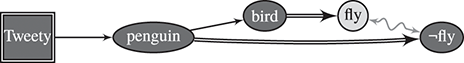
Example 3 (Tweety; Doyle and McDermott (1980)). Another well-known example is Tweety the penguin (see Fig. 2) based on the following information:
- 1. Tweety is a penguin.
- 2. Penguins are birds.
- 3. By default, birds fly.
- 4. By default, penguins don’t fly.

 and (b)
  . According to the specificity principle more specific defaults such as
  are prioritized over less specific ones, such as
  . The reason is that more specific defaults may express exceptions to the more general ones. So, in this example the preferred outcome
  will be obtained since the less specific defeasible argument (a) should be retracted in favor of (b).
Figure 1 The Nixon Diamond from Example 2. Double arrows symbolize defeasible rules, single arrows strict rules, and wavy arrows conflicts. Black nodes represent unproblematic conclusions, while light nodes represent problematic conclusions. Rectangular nodes represent the starting point of the reasoning process. We use the same symbolism in the following figures.

Figure 2 Tweety and specificity, Example 3.
Figure 2Long description
A single arrow from penguin leads to bird (black node). A double arrow from penguin leads to ¬ fly (black node) and from bird leads to fly (light node). A way arrow is drawn between fly and ¬fly.
Our examples indicate that, first, conflicts between defeasible arguments can occur, and second, the context may determine whether and, if so, how a conflict can be resolved. We now take a look at two further challenges that come with conflicts in defeasible reasoning.
Figure 3 encodes the following information:  ,
,  ,
,  , and
, and  . Should we infer
  ? Nonmonotonic logics that block this inference have been said to suffer from the drowning problem (Benferhat et al., Reference Benferhat, Cayrol, Dubois, Lang and Prade1993). Examples like the following seem to suggest that we should accept
  .
.

Figure 3 A drowning scenario.
Example 4. We consider the scenario:
- 1. Micky is a dog.
- 2. Dogs normally (have the ability to) to tag along with a jogger.
- 3. Dogs normally (have the ability to) bark.
- 4. Micky lost a leg and can’t tag along with a jogger.


In this example it seems reasonable to infer,  , Micky has the ability to bark, despite the presence of
  . In other contexts one may be more cautious when jumping to a conclusion.
Example 5. Take the following scenario.
- 1. It is night.
- 2. During the night, the light in the living room is usually off.
- 3. During the night, the heating in the living room is usually off.
- 4. The light in the living room is on.


In this scenario it seems less intuitive to infer,  , The heating in the living room is off. The fact that we have in (4) an exception to default (2) may have an explanation in the light of which also default (3) is excepted. For example, the inhabitant forgot to check the living room before going to sleep, she is not at home and left the light and heating on before leaving, she is still in the living room, and so on.
These examples show that concrete reasoning scenarios often contain a variety of relevant factors that influence what real-life reasoners take to be intuitive conclusions. Specific NMLs typically only model a few of these factors and omit others. For instance, although Elio and Pelletier (Reference Elio and Pelletier1994) and Koons (Reference Koons and Zalta2017) argue that it is useful to track causal and explanatory relations in the context of drowning problems, systematic research in this direction is lacking.
Another class of difficult scenarios has to do with so-called floating conclusions.Footnote 10
These are conclusions that follow from two opposing arguments. For example, formally the scenario may be as depicted in Fig. 4.

Figure 4 A scenario with the floating conclusion  .
.
Example 6. Suppose two generally reliable weather reports:
- 1. Station 1: The hurricane will hit Louisiana and spare Alabama.
- 2. Station 2: The hurricane will hit Alabama and spare Louisiana.
- 3. If the hurricane hits Louisiana, it hits the South coast.
- 4. If the hurricane hits Alabama, it hits the South coast.


The floating conclusion, (5), The storm will probably hit the South coast, may seem acceptable to a cautious reasoner. The rationale being that both reports agree on the upcoming storm and even roughly where it will hit. The disagreement may be due to different weighing of diverse factors in their respective underlying scientific weather models. But the combined evidence of both stations seems to rather confirm conclusion (5) than dis-confirm it. This is not always the case with partially conflicting expert statements, as the next example shows.
Example 7. Assume two expert reviewers, Reviewer 1 and Reviewer 2, evaluating Anne for a professorship. She sent in two manuscripts, A and B.
- 1. Reviewer 1: Manuscript A is highly original, while manuscript B repeats arguments already known in the literature.
- 2. According to Reviewer 1, one manuscript is highly original.
- 3. Reviewer 2: Manuscript B is highly original, while manuscript A repeats arguments already known in the literature.
(We assume the inconsistency of
with .)- 4. According to Reviewer 2, one manuscript is highly original.


Should we conclude that one manuscript is highly original, since it follows from both reviewers’ evaluations? It seems a more cautious stance is advisable. The disagreement may well be an indication of the sub-optimality of each of the two reviews. Indeed, a possible explanation of their conflicting assessments could be that (a) Reviewer 1 is aware of an earlier article  (by another author than Anne) that already makes the arguments presented in
  and which is not known to Reviewer 2, and vice versa, that (b) Reviewer 2 is aware of an earlier article
  in which similar arguments to those in
  are presented. In view of this possibility, it would seem overly optimistic to infer that Anne has a highly original article in her repertoire.
2 Central Concepts
Nonmonotonic logics are designed to answer the question what are (defeasible) consequences of some available set of information. This gives rise to the notion of a nonmonotonic consequence relation. In this section we explain this central concept and some of its properties from an abstract perspective (Section 2.2). Nonmonotonic consequences are obtained by means of defeasible inferences, which are themselves obtained by applying inference rules. We discuss two ways of formalizing such rules in Section 2.3. Before doing so, we discuss some basic notation in Section 2.1.
2.1 Notation and Basic Formal Concepts
Let us get more formal. We assume that sentences are expressed in a (formal) language  . We denote the standard connectives in the usual way:
  (negation),
  (conjunction),
  (disjunction),
  (implication), and
  (equivalence). We use lowercase letters
  as propositional atoms, collected in the set
  , and uppercase letters
  as metavariables for sentences such as
  ,
,  or
or  . We denote the set of sentences underlying
  by
by  . In the context of classical propositional logic and typically in the context of a Tarski logic (see later), this will simply be the closure of the atoms under the standard connectives.Footnote 11 We denote sets of sentences by the uppercase calligraphic letters
  ,
,  , and
, and  . Where
  is a finite nonempty set of sentences, we write
  and
and  for the conjunction resp. the disjunction over the elements of
  .Footnote 12
A consequence relation, denoted by  , is a relation
  between sets of sentences and sentences:
  denotes that
  is a
is a  -consequence of the assumption set
  . So, the right side of
  encodes the given information resp. the assumptions on which the reasoning process is based, while the left side encodes the consequences which are sanctioned by
  given
given  .
.
We will often work in the context of Tarski logics  , whose consequence relations
  are reflexive (
 ), transitive (
 and
and  implies
  ) and monotonic (Definition 2.1). We will also assume compactness (if
  then there is a finite
  for which
  ). The most well-known Tarski logic is, of course, classical logic
  .
.
2.2 An Abstract View on Nonmonotonic Consequence
The following definition introduces one of our key concepts: nonmonotonic consequence relations.
Definition 2.1. A consequence relation  is monotonic iff (“if and only if”) for all sets of sentences
  and
and  and every sentence
  it holds that
  if
if  . It is nonmonotonic iff it is not monotonic.
We use  as a placeholder for nonmonotonic consequence relations. Our definition expresses that for nonmonotonic consequence relations
  there are sets of sentences
  and
and  for which
  while
while  (i.e.,
  is not a
  -consequence of
  ).
).
In the following we will introduce some properties that are often discussed as desiderata for nonmonotonic consequence relations.Footnote 13 A positive account of what kind of logical behavior to expect from these relations is particularly important given the fact that ‘nonmonotonicity’ only expresses a negative property. This immediately raises the question whether there are restricted forms of monotonicity that one would expect to hold even in the context of defeasible reasoning? One proposal is
- Cautious Monotonicity (CM).
- , if and .Footnote 14


Whereas nonmonotonicity expresses that adding new information to one’s assumptions may lead to the retraction resp. the defeat of previously inferred conclusions, CM states that some type of information is safe to add: namely, adding a previously inferred conclusion does not lead to the loss of conclusions.
We sketch the underlying rationale. Suppose  and
and  . In view of
  , the defeasible consequence
  of
of  is sanctioned. So,
  does not contain defeating information for concluding
  . Now, the only reason for
  would be that the addition of
  to
to  generates defeating information for concluding
  . However,
  already followed from
  , since
  . Thus, this defeating information should have already been contained in
  , before adding
  . But then
  , a contradiction.
One may also demand that adding  -consequences to an assumption set should not lead to more consequences.
- Cautious Transitivity (CT).
- , if and .


Combining CM and CT comes down to requiring that  is robust under adding its own conclusions to the set of assumptions.
- Cumulativity (C).
If
, then iff .


Instead of considering the dynamics of consequence under additions of new assumptions, one may wonder what happens when assumptions are manipulated. For instance, it seems desirable that a consequence relation is robust under substituting assumptions for equivalent ones.
- Left Logical Equivalence (LLE).
Where
and are classically equivalent sets,Footnote 15 iff .


Note that in the context of nonmonotonic consequence it would be too strong to require
- Left Logical Strengthening (LLS).
Where
, implies .


In order to see why LLS is undesirable, consider an example featuring Tweety. If it is only known that Tweety is a bird, it nonmonotonically follows that it can fly,  . The situation changes when it is also known that Tweety is a penguin,
  .
.
For the right-hand side of  one may also expect a property similar to LLE: if
  is a consequence, so is each equivalent formula
  . The following principle is stronger. It is motivated by the truth-preservational nature of CL-inferences (but recall from Section 1.2 that in the context of generics it may be problematic):
- Right Weakening (RW).
Where
, implies .


Finally, if we take our assumptions to express certain information (rather than defeasible assumptions, see Section 4), then one may expect
- Reflexivity (Ref).
- .

Consequence relations that satisfy RW, LLE, Ref, CT, and CM are called cumulative consequence relations (Kraus et al., Reference Kraus, Lehman and Magidor1990).Footnote 16 The authors consider them “the rockbottom properties without which a system should not be considered a logical system.” (p. 176), a point mirroring Gabbay (Reference Gabbay and Apt1985). Some other intuitive principles hold for a cumulative  .
.
Proposition 2.1. Every cumulative consequence relation  also satisfies:
1. Equivalence. If
and then: iff .2. AND. If
and then .


Proof. Item 1 follows by CT and CM. To see this suppose (a)  , (b)
, (b)  , and (c)
  . We show
  (the inverse direction is analogous). By CM, (a) and (c),
  . Thus, by CT and (b),
  .
.
Ad 2. Suppose (a)  and (b)
  . By Ref,
  and by LLE, (c),
  . By CM, (a) and (b),
  . By CT and (c),
  . By (a) and CT,
  . □
. □
Another property of some NMLs is constructive dilemma: given a fixed context represented by  , if
, if  is both a consequence of
  and of
  , it should also be a consequence of
  .
.
- Constructive Dilemma (OR)
If
and then .


Cumulative consequence relations that also satisfy OR are called preferential (Kraus et al., Reference Kraus, Lehman and Magidor1990). We show some derived principles for preferential consequence relations.
Proposition 2.2. Every preferential consequence relation  also satisfies:
1. Reasoning by Cases (RbC). If
and then .2. Resolution. If
then .


Proof. (RbC). Suppose  and
and  . By OR,
  and by LLE,
  . (Resolution). Suppose now that
  . By RW, (a),
  . By Ref,
  and by RW, (b),
  . By RbC, (a) and (b),
  . □
. □
A more controversial property than CM is rational monotonicity (RM).Footnote 17 The basic intuition is similar to CM: given an assumption set  , we are interested in securing a safe set of sentences under the addition of which
  is monotonic. While for CM this was the set of the
  -consequences of
  , RM considers the set of all sentences that are consistent with the consequences of
  (consistent in the sense that their negation is not a
  -consequence of
  ).
).
- Rational Monotonicity (RM)
- , if and .


One way to think about RM is as follows. Let us (i) say that  is defeating information for
  if there is an
  for which
  , while
  , and (ii)
  is rebutted by
  in case
  .Footnote 18 Then, when putting CM and RM in contrapositive form,
CM expresses that no defeating information for
is derivable from any : formally, if and then ;RM expresses the stronger demand that every defeating information for
is rebutted by : formally, if and then .


So, RM requires that reasoners take into account potentially defeating information by having rebutting counterarguments at hand. This is quite demanding, since, as we have discussed in Section 1, (a) the reasoner may not be aware of all possibly rebutting information to her previous inferences and (b) it may be counterintuitive to conclude that each and every possible defeater is false.
Poole (Reference Poole1991) points out another problem. Consider the statement that Tweety is a bird. Now, all bird species are exceptional to some defaults about birds: penguins don’t fly, hummingbirds have an unusual size, sandpipers nest on the ground, and so on. But, then RM requires us to infer that Tweety is not a penguin, not a hummingbird, not a sandpiper, and so on, and therefore does not belong to any bird species.
In this section we have seen various properties of nonmonotonic consequence relations, many of which are considered desiderata by nonmonotonic logicians. Their study is therefore of central interest in NML and we will come back to them in the context of many of the methods presented in this Element.
2.3 Plausible and Defeasible Reasoning
A fundamental question underlying the design of NMLs is whether to model defeasible reasoning
1. by means of classical inferences based on defeasible assumptions, or
2. by means of (genuinely) defeasible inference rules.
The former is sometimes called Plausible Reasoning, the latter Defeasible Reasoning.Footnote 19 Table 1 provides an overview on which of the two reasoning styles is modeled by various NMLs discussed in this Element. We illustrate with an abstract example. Suppose we want to model that
- defeasibly implies , and that
- defeasibly implies .


In the first approach we encode these two defeasible regularities in terms of classical implications. It can be realized in two ways.
Plausible Reasoning via abnormality assumptions. One way is by formalizing the defeasible rules by

where  and
and  are atomic sentences that encode exceptional circumstances, that is, abnormalities, for the respective rules. These abnormalities are assumed to be false, by default. Suppose that
  is true. Then, by also assuming the falsity of
  and
and  we can apply modus ponens to both material implications and conclude
  .
.

Table 1Long description
The table consists of four columns: NML, Defeasible Reasoning, Plausible Reasoning, and Blank. It read as follows. Row 1: ASPIC plus; checkmark in Defeasible Reasoning; checkmark in Plausible Reasoning; Section 8. Row 2: Logic-based argumentation; checkmark in Plausible Reasoning; Section 9. Row 3: Rescher and Manor; checkmark in Plausible Reasoning; Section 11 dot 3 dot 1. Row 4: Default Assumptions; checkmark in Plausible Reasoning; Section 11 dot 3 dot 1. Row 5: Adaptive Logic; checkmark in Plausible Reasoning; Section 11 dor 3 dot 1. Row 6: Input-Output Logic; checkmark in Defeasible Reasoning; checkmark in Plausible Reasoning with asterisk; Section 11 dot 3 dot 2. Row 7: Reiter Default Logic; checkmark in Defeasible Reasoning; checkmark in Plausible Reasoning with asterisk; Section 12. Row 8: Logic Programming; checkmark in Plausible Reasoning; Section 16.
Let us see how retraction works in this approach by supposing  . In this case we can classically derive
  , but neither
  nor
nor  . Note that contraposition of defeasible rules is available in this approach. For instance,
  is CL-equivalent to
  .Footnote 20 So, we know (at least) one of the assumptions must be false, but we don’t know which. Absent any other reason to prefer one over the other, we can’t rely on
  to derive
  . In view of this,
  should not be considered a nonmonotonic consequence of the given information.
Plausible Reasoning via naming of defaults. Another way to proceed is by naming defaults (see, e.g., Poole (Reference Poole1988)). Here, we make use of defeasible assumptions  and
and  , which name defeasible inference rules and which are assumed to be true, by default. In our example, we add

to the (nondefeasible) assumptions. Note that  (resp.
  ) is classically equivalent to
  (resp.
  ). So, when substituting
  for
for  and
and  for
for  the approach based on naming defaults and the approach based on abnormality assumptions boil down to the same.
Defeasible Reasoning. In this approach, regularities are expressed as genuinely defeasible rules (written with  ), that is, without additional and explicit defeasible assumptions that are part of the antecedent of the rule. We encode our preceding example by

Note that  is not classical implication, in particular
  does, in general, not follow from
  in this approach. In the first scenario, where only
  is given, we apply a defeasible modus ponens rule to obtain
  and then again to obtain
  . Many NMLs implement a greedy style of reasoning, according to which defeasible modus ponens is applied as much as possible. Now, if
  is also part of the assumptions, we derive
  from
from  and
and  , but then stop, since inferring
  from
from  and
and  would result in inconsistency.
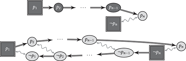
Example 8. For a more general context, we consider an example with defaults  and the (certain) information
  and
and  depicted in Figure 5. In the greedy style of reasoning underlying Defeasible Reasoning we will be able to apply defeasible modus ponens to derive
  ,
,  , …,
, …,  . Only the last application resulting in
  is blocked by the defeating information
  . The situation is different for Plausible Reasoning. Since contraposition is available, for each argument
  (where each
  is modeled by
  ) there is a defeating argument
  . Altogether, we obtain

This means that at least one  cannot be assumed to be false, but we don’t know which one. Thus, no
  (for
(for  ) is derivable according to Plausible Reasoning.

Figure 5 Top: Defeasible Reasoning giving rise to a greedy reasoning style. Bottom: Plausible Reasoning giving rise to contrapositions of defeasible rules.
3 From Knowledge Bases to Consequences and NMLs
Nonmonotonic logics represent the information relevant for the reasoning process (knowledge representation) and determine what follows defeasibly from the given information (nonmonotonic consequence, see Fig. 6).

Figure 6 The workings of NMLs.
The task of knowledge representation concerns, for instance, the structuring of the starting point of defeasible reasoning processes in terms of knowledge bases (Section 4) in which different types of information are distinguished, such as different types of assumptions and inference rules. Another task is to organize the given information in a way that is conducive of determining its defeasible consequences. As we have seen, this is challenging since the given information may give rise to conflicts and inconsistencies. NMLs provide methods for generating coherent chunks of information. We will highlight several ways of doing so, most roughly distinguished into syntactic and semantic approaches. The following three concepts play essential roles in the ways knowledge is represented in these approaches:Footnote 21
- Extensions
In syntactic approaches, coherent units of information are typically called extensions. What exactly extensions are differs in various NMLs. They may, for example, be sets of defeasible information from the knowledge base, sets of arguments (given a underlying notion of argument), or sets of sentences. In Section 5.1, 5.2 we will introduce two major families of syntactic approaches: argumentation and consistent accumulation. In Parts II and III they will be studied in more detail.
- Arguments
In syntactic approaches, arguments (or proofs) play a central role when building extensions. Arguments are obtained by applications of the given inference rules to the assumptions provided in the knowledge base.
- Models
In semantic approaches the focus is on classes of models provided by a given base logic. In Section 5.3 we will introduce semantic approaches and study some of them in more detail in Part IV.
The attentive reader will have noticed that we did not yet define what exactly NMLs are. In the narrow sense, one may consider them as nonmonotonic consequence relations (see Section 2.2), so a theory of what sentences follow defeasibly in the context of some knowledge base. In the wider sense they are methods for both knowledge representation and for providing nonmonotonic consequence relation(s).
In this Element we minimally assume that every NML  comes with a formal language
  including a notion of what counts as a formula or sentence (written
  ), an associated class of knowledge bases
  (see Section 4 for details), at least one consequence relation and one of the following two:
in syntactic approaches: a notion of (in)consistent sets of sentences, of argument or proof, and a method to generate extensions (see Sections 5.1 and 5.2 and Parts II and III);
in semantic approaches: a notion of model and a method to select models (see Section 5.3 and Part IV).
4 Defeasible Knowledge Bases
Reasoning never starts in a void but it is initiated in a given context. For instance, some information will be factually given and some assumptions may hold by default. Moreover, when we reason we make use of inference rules. Some of these may be truth-preservational (such as the rules provided by  ), others defeasible, allowing for exceptional circumstances. Defeasible knowledge bases structure reasoning contexts into different types of constituents, such as different types of assumptions and inference rules. Most broadly conceived they are tuples of the form:
 (4.0.1)
We let  be the defeasible part of
  consisting of its defeasible assumptions and rules.
A concrete  has an associated fixed class of knowledge bases
  . Its underlying consequence relation(s)
  are relations between
  and
and  .Footnote 22
In concrete NMLs, usually not all components of (4.0.1) are utilized or explicitly listed. For example, some NMLs do not consider defeasible rules, some come without defeasible assumptions, some without priorities, many without metarules. Take, for instance, NMLs that model Plausible Reasoning. Here, we omit  since such NMLs do not work with defeasible rules. Moreover, specific components of the knowledge base are fixed for many NMLs, or they are constrained. For instance, only specific preferences relations
  may be allowed for, such as transitive ones. Or, often the strict rules are induced by classical logic. (In such cases, the strict rules are often omitted from
  .) In some NMLs the strict rules vary over different applications (e.g., in logic programming where strict rules usually represent domain-specific knowledge such as “penguins are birds”). In Table 2 we provide an overview for NMLs presented in this Element.

Table 2Long description
The table with seven columns titled: NML, A subscript s, A subscript d, R subscript s, R subscript d, R subscript m, and Section. The rows read as follows: Row 1: ASPIC plus, tick in A subscript s, A subscript d, R subscript s, and R subscript d; Section 8. Row 2: Logic-based argumentation, tick in A subscript s and A subscript d, tick with R subscript L in R subscript s; Section 9. Row 3: Rescher and Manor: tick in A subscript d, tick in R subscript CL in R subscript s; Section 11 dot 3 dot 1. Row 4: Default Assumptions, tick in A subscript s and A subscript d, tick with R subscript CL in R subscript s; Section 11 dot 3 dot 1. Row 5: Input-output logics, tick in A subscript s, tick with R subscript CL in R subscript s; tick in R subscript d and tick mark in R subscript m; Section 11 dot 3 dot 2. Row 6: Reiter Default Logic, tick in A subscript s, tick with R subscript CL in R subscript s, tick in R subscript d; Section 12. Row 7: Logic Programming, tick in R subscript s; Section 16.
We now explain in more detail the components of  .
.
- Strict assumptions
- is a set of sentences expressing information that is taken as indisputable or certain.
- Defeasible assumptions
- is a set of sentences that are assumed to hold normally/typically/and so on but which may be retracted in case of conflicts.
- Strict rules
- is a set of truth-preservational inference rules or relations, written .Footnote 23 There are two types of such rules. On the one hand, we have material inferences, such as “If it is a penguin, it is a bird” which may be encoded by . On the other hand, we have inferences that are valid with respect to an underlying logic , such as classical logic. If such inferences are considered, we let if . If consist exclusively of such rules, we say that it is induced by the logic and write for the set containing them. All logics considered in this Element will be Tarski logics. If is induced by a logic (with an implication ) one may model the former class of material inferences simply by means of . For example, in our example one may add to the strict assumptions . Sometimes we find strict assumptions being modeled as strict rules with empty bodies .
Given a set of strict rules
and a set of sentences , we write to indicate that there is a deduction of based on and . This means that there is a sequence where and for each (with ), either or there are for which . - Defeasible rules
- is a set of defeasible inference rules written , often just called defaults. As discussed in Section 2.3, defeasible rules are sometimes “indirectly” modeled as strict rules with defeasible assumptions. In NMLs that adopt this method of Plausible Reasoning, may be empty. In such cases we are typically dealing with a logic-induced set of strict rules and defaults are sentences of the type in where . Defeasible assumptions may be also considered as defaults with empty bodies.


For reasons of simplicity and following the tradition of many central NMLs, we do not consider  as a defeasible conditional operator in the object language
  , that is, an operator that can be nested within Boolean connectives. Rather, we model
  as representing a defeasible rule that prima facie justifies detaching
  , given
  . However, it should be noted that this does impose a limitation on our expressive capabilities. For instance, we cannot “directly” express canceling in the context of specificity, such as
  . Many systems have been developed to overcome this limitation, such as Delgrande (Reference Delgrande1987) or conditional logics of normality (Boutilier, Reference Boutilier1994a).Footnote 24
Example 9. In Section 2.3 we presented two ways to model a scenario in which  defeasibly implies
  and
and  defeasibly imply
  . Suppose now additionally that
  and
and  both strictly imply
  and that
  defeasibly implies
  .
.
In Defeasible Reasoning we may work with the knowledge base 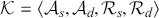 consisting of
  ,
,  ,
,  , and
, and  . Alternatively, one may use the strict assumptions
  and
and  and
and  as strict rules.
In Plausible Reasoning we may utilize  , where
  and
and  .
.
- Metarules
- is a set of metarules, written (where are strict and defeasible rules and is a defeasible rule) that allow one to infer new defeasible rules from those in and . For example, metarules implementing reasoning-by-cases and right weakening are:
- OR
- RW
Given a set
, we write for the set of defeasible rules that are -deducible from by the metarules in (where deductions are defined as in the context of the strict rules ).Footnote 25- Preferences
- is an order on the defeasible elements of . It encodes that some sources of defeasible information may be more reliable or have more authority than others. This information can be utilized for the purpose of resolving conflicts between defeasible arguments of different strengths. Typically is reflexive and transitive, but it may allow for incomparabilities and for equally strong but different defeasible elements. We write for the strict version of , that is, iff and .


Example 10.
Consider  with
with  and
and  . There is a conflict between the arguments
  and
and  . Absent priorities, there is no way to resolve the conflict on the basis of
  . If we enhance
  to
to  where
where  it seems reasonable to resolve the conflict in favor of
  .
.
The situation can get more involved, as the following example shows.
Example 11 (Example 9 cont.). We may extend our knowledge base to  by adding the preference order:
  (assuming transitivity).Footnote 26 In this case we have two conflicting arguments,
  and
and  . Comparing their strengths is no longer straightforward, since the former involves both a stronger and a weaker default than the latter. In Part III (Examples 28 and 29) we will see that different methods give rise to different conclusions for
  (see also Liao et al. (Reference Liao, Oren, van der Torre, Villata, Cariani, Grossi, Meheus and Parent2016)).
5 Methodologies for Nonmonotonic Logics
We now introduce three central methodologies to obtain nonmonotonic consequence relations and to represent defeasible knowledge, namely: formal argumentation (Section 5.1), consistent accumulation (Section 5.2), and semantic methods (Section 5.3). In this part we explain basic ideas underlying each method based on simplified settings (e.g., without metarules and preferences). More details are presented in the dedicated Parts II to IV.
5.1 The Argumentation Method
The possibility of inconsistency complicates the question as to what follows from a knowledge base  . As described earlier, the idea is to generate coherent sets of information from
  and to reason on the basis of these. For this, arguments and attacks between them play a key role. Arguments are obtained from
  by chaining strict and defeasible inference rules. We can define the set of arguments
  induced by
  , their conclusions, subarguments, and defeasible elements (written
  ,
,  , resp.
  for some
  ) in a bottom-up way.Footnote 27
Definition 5.1 (Arguments). Where  is a knowledge base we let
  iff
iff
- , where .
We let
, , , . - where , and is a rule in .
We let
, , , .


Where  we let
  . Where
  , we let
  be the set of all
  for which
  .
.
Example 12 (Example 9 cont.). Given our knowledge base  in Example 9 we obtain the arguments depicted in Fig. 7 (left). We have, for instance,
  ,
,  , and
, and  .
.

Figure 7 The arguments and the argumentation framework for Example 13 (omitting the nonattacked and nonattacking  and
and  ). We explain the shading in Example 14.
There are many ways to define argumentative attacks and subtlety is required to avoid problems with consistency in the context of selecting arguments. We will go into more details in Part II. For now we simply suppose there to be a relation  that determines when two arguments attack each other. We end up with a directed graph
  , a so-called argumentation framework (Dung, Reference Dung1995).
Example 13 (Example 12 cont.). One way to define attacks in our example is to let  attack
  if for some
  of the form
  ,
,  or
or  . For instance,
  and
and  attack each other. In Fig. 7 (right) we find the underlying argumentation framework.
Argumentation frameworks allow us to select coherent sets of arguments  , which we will call A-extensions (for argumentative extensions). The latter represent argumentative stances of rational reasoners equipped with the knowledge base
  . For this we utilize a number of constraints which represent rational desiderata on these stances. Two such desiderata on sets of arguments
  are, for instance (we refer to Part II for a more comprehensive overview):
- Conflict-freeness:
avoid argumentative conflicts, that is, for all
, ; and- Stability:
additionally, be able to attack arguments that you don’t commit to, that is, for all
there is an for which .


Such sets of constraints give rise to so-called argumentation semantics which determine A-extensions of a given argumentation framework (Dung, Reference Dung1995). For instance, according to the stable semantics the set of A-extensions is the set of all sets of arguments that satisfy stability. Once we have settled for an argumentation semantics  (such as the stable semantics) we denote the set of A-extensions of
  relative to
  by
by  .
.
Example 14 (Example 13 cont.). We have two stable A-extensions, that is, sets of arguments that satisfy the stability requirement (see the shaded sets in the argumentation framework of Fig. 7):

Suppose we select an A-extension  . We then commit to all of the conclusions of the arguments in
  , that is, to
  , where
  . This induces another notion of extension, which we dub P-extensions (propositional extensions) which are sets of conclusions associated with A-extensions. We write
  for the set of P-extensions of
  (relative to a given argumentation semantics
  ).
).
Example 15 (Example 14 cont.). The following P-extensions are associated with our A-extensions:

Once an argumentation semantics is fixed and the A- and corresponding P-extensions are generated, we can define three different consequence relations for two underlying reasoning styles (see Fig. 8): skeptical and credulous reasoning.

Figure 8 The skeptical and the credulous reasoning style.
Figure 8Long description
The diagram depicts the following: Defeasible knowledge base leads to build extensions which further leads to 1. Sceptical approach: infer A if it is supported in every extension and 2. Credulous approach: infer A if it is supported in some extension by some argument |~ ∪Ext. Sceptical approach further leads to 1. by some argument (conclusion-focused) |~ ∩PExt and 2. by the same argument (argument-focused) |~∩AExt. Both of which further lead to floating conclusion.
Definition 5.2. Where  is a knowledge base,
  a sentence, and
  is an argumentation semantics, we define the consequence relations in Table 3.

Table 3Long description
The table consists of two columns. It read as follows: Row 1: Skeptical 1: K turnstile superscript S subscript intersection P-extensions A iff A element of intersection P-extensions subscript S (K), A is a member of every extension in P-extensions subscript S (K). Row 2: Skeptical 2: K turnstile superscript S subscript intersection A extensions A iff there is an a element A-extensions subscript S (K) s. t. Con (a) equals A, There is an argument a with Con (a) equals A that is contained in every A-extension of K. Row 3: Credulous: K turnstile superscript S subscript union extensions A iff A element of union P extensions subscript S (K), A is a member of some extension in P-extensions subscript S (K).
To avoid clutter in notation, we will omit the super- and subscripts whenever the context disambiguates or the strategy is not essential to a given claim. Note that the definition of the three consequence relations imposes a hierarchy in terms of strength, namely:

Example 16 (Example 15 cont.). Based on our extensions, we have the following consequences:

Table 016Long description
The table consists of five columns: p, q, not r, r, and s. It reads as follows: Row 1: Turnstile intersection P extensions: tick in p, tick in q, blank in not r and r, tick in s. Row 2: Turnstile intersection A extensions: tick in p and q; blank in not r, r, and s. Row 3: Turnstile union extensions: tick in all columns - p, q, not r, r, and s.
The example illustrates that a floating conclusion such as  follows by
  but not by the more cautious
  .
.
5.2 Methods based on Consistent Accumulation
Given a knowledge base  , the basic idea behind the accumulation methods is to iteratively build coherent sets of defeasible elements from
  .Footnote 28 We will call such sets D-extensions (extensions consisting of defeasible elements). Below we identify two central methods of building D-extensions: the greedy and the temperate method. Once D-extensions have been generated by one of these methods, we can associate each D-extension
  with an A-extension
  consisting of all the arguments based on elements in
  . Moreover, each A-extension
  has the corresponding P-extension
  as discussed in Section 5.1. Once A- and P-extensions are obtained, we define consequence relations just like in Definition 5.2 (see the overview in Fig. 9). We now discuss the two types of accumulation methods.

Figure 9 Types of nonmonotonic consequence based on syntactic approaches.
Figure 9Long description
Both a. and b. leads to extensions which further leads to 1. Skeptical consequence and 2. Credulous consequence. Skeptical consequence leads to |~ ∩PExt and |~ ∩AExt. Credulous consequence leads to |~ UExt.
5.2.1 The Greedy Method
Given a knowledge base  , methods based on consistent accumulation build iteratively sets of defeasible elements from
  . One may think of a rational agent that extends her commitment store
  consisting of elements in
  in a stepwise manner. She starts off with the empty set and in each step she adds an element of
  to
to  or she stops the procedure. She stops when adding any new element
  would lead to inconsistency, that is, in case she would be able to construct conflicting arguments on the basis of
  .
.
According to the greedy method, she will only consider adding elements in  to her commitment store that (a) give rise to new arguments (that is the greedy part) and (b) do not give rise to conflicting arguments. We will make this formally precise with the algorithm GreedyAcc in what follows, but we first need to introduce some concepts. Where
  , we say that a default
is triggered by
, if ,Footnote 29is consistent with
, if .


If  is triggered by
  , adding
  to
to  gives rise to new arguments in
  . The reason for this is that for each
  (with
(with  ) there is an argument
  with conclusion
  , and
, and  . We treat defeasible assumptions
  like defaults with empty left-hand sides: they are always triggered, and consistent with
  only if
  .
.
The algorithm GreedyAcc implements the greedy accumulation method. We note that the element  in lines 3 and 4 is chosen nondeterministically.

Algorithm 1Long description
The Algorithm displays seven lines: 1. procedure Greedy Accumulation (K); K equals A subscript s, A subscript d, R subscript s, R subscript d. 2. Defeasible asterisk left arrow empty set; init scenario. 3. while exists d element of Defeasible (K) backslash Defeasible asterisk triggered by and consistent with Defeasible asterisk do. 4. Defeasible asterisk left arrow Defeasible asterisk union {d}; update scenario. 5. end while; no more triggered and consistent defaults. 6. return Defeasible asterisk; return D-extension. 7. end procedure.
GreedyAcc takes as input a knowledge base  and outputs a D-extension
  . Its associated A-extension is given by
  and its associated P-extension by
  . The latter can be used to determine our three consequence relations from Definition 5.2. We write
  [resp.
  ,
,  ] for the set of D-[resp. A-, P-]extensions of
  (
( for greedy accumulation). We are now in a position to define three consequence relations analogous to Definition 5.2 (see Table 3), for example, by:

Example 17 (Example 12 cont.). We apply GreedyAcc to the given knowledge base  . There are three different runs (due to the nondeterministic nature of the algorithm):

Table 01Long description
The table consists of three columns titled: Run 1, Run 2, and Run 3. Row 1: Round 1: p implies r; p implies q; p implies q. Row 2: Round 2: p implies q; p implies r; q implies not r. Row 3: P-extension: set of p, r, q, and s; set of p, r, q, and s; set of p, not r, q, and s. Row 4: A-extension: set of a subscript 1, a subscript 2, a subscript 4, and a subscript 6; set of a subscript 1, a subscript 2, a subscript 4, and a subscript 6; set of a subscript 1, a subscript 2, a subscript 3; set of a subscript 5.
Next we list consequences according to the three different consequence relations:

Table 02Long description
The table consists of five columns: p, q, not r, r, and s. It reads as follows: Row 1: Turnstile intersection P-extension, tick in columns p, q, and s. Row 2: Turnstile intersection A-extension, tick in columns p and q. Row 3: Turnstile union extension, tick in columns p, q, not r, r, and s.
Note that for  we have to consider the intersection of all P-extensions
  and so we get the floating conclusion
  (just like in Example 16). For
  we consider the intersection of the A-extensions
  : while
  the floating conclusion
  is not in
  . Finally, for
  we consider the union of all P-extensions
  .
.
5.2.2 Temperate Accumulation
Our second accumulation method is nongreedy (or, temperate) in that the defeasible elements from  that may be added to the commitment store
  in each step of the algorithm can be such that they don’t give rise to new arguments. In more technical terms, our agent may also add defeasible rules which are not triggered by
  . This is described in Algorithm 2, TemAcc. We use the same notation as before:
  is the set of D-extensions generated by TemAcc(
 ) and
) and  resp.
resp.  is the corresponding set of A- resp. P-extensions. The three types of consequence relations
  ,
,  , and
, and  are defined analogously to the greedy versions (see Table 3).

Algorithm 2Long description
The Algorithm displays seven lines: 1. Procedure Temperate accumulation (K). 2. Defeasible asterisk left arrow empty set, init scenario. 3. while exists d element of Defeasible (K) backslash Defeasible asterisk consistent with Defeasible asterisk do. 4. Defeasible asterisk left arrow Defeasible asterisk union {d}, update scenario. 5. end while, no more consistent defaults. 6. return Defeasible asterisk, return D-extension. 7. end procedure.
Remark 1. Let us make two immediate observations to better understand how the greedy approach relates to the temperate approach. First, since defeasible assumptions are always triggered, the greedy and the temperate accumlation methods coincide for knowledge bases without defeasible rules (where  ). Second, every run via GreedyAcc corresponds to the initial segment of some runs via TemAcc.
Example 18 (Example 17 cont.). We apply TemAcc to our knowledge base. There are six possible runs, omitting runs 1–3 which are analogous to Example 17:

Table 03Long description
The table consists of three columns titled: Run 4, Run 5, and Run 6. Row 1: Round 1: q implies not r; q implies not r; p implies r. Row 2: Round 2: p implies q; p implies r; q implies not r. Row 3: P-extension: set of p, not r, q, and s; set of p, r, and s; set of p, r, and s. Row 4: A-extension: set of a subscript 1, a subscript 2, a subscript 3, and a subscript 5; set of a subscript 1, a subscript 4, and a subscript 6; set of a subscript 1, a subscript 4, and a subscript 6.
In comparison with GreedyAcc we get three additional runs, namely 4–6. While run 4 is just a permutation of run 3, runs 5 and 6 give rise to new D-extensions. They show the nongreedy character of TemAcc. Consider, for instance, run 6: although in round 2 the default  is both triggered and consistent with
  , the algorithm chooses the nontriggered
  .
.
We list consequences according to the different notions of consequence, marking differences to GreedyAcc with [!]:

Table 04Long description
The table consists of five columns titled: p, q, not r, r, and s. Row 1: Turnstile intersection P-extension, tick in columns p and s; exclamation mark in column q; columns not r and r are empty. Row 2: Turnstile intersection A-extension, tick in column p; exclamation mark in column q; columns not r, r, and s are empty. Row 3: Turnstile union extension, tick in all five columns - p, q, not r, r, and s.
We see that  does not follow anymore by
  and
and  .
.
While in our example every D-extension based on greedy accumulation is also one based on temperate accumulation, the example demonstrates this typically doesn’t hold vice versa. As a consequence, temperate accumulation gives rise to a more cautious style of reasoning than the greedy approach, at least in terms of the skeptical consequence relations and when there are no preferences involved (see Example 29 for a counterexample with preferences).
Figure 10 gives an overview on NMLs discussed in this Element and where they fall in terms of our classification.

Figure 10 The syntactic approach and NMLs discussed in this Element.
Figure 10Long description
Argumentation, Part Two further leads to A S P I C and logic-based. Accumulation, Part Three branches into 1. temperate, Chapter 11, which further leads to M C S-based reasoning and input/output logic and 2. greedy, Chapter 12, which further leads to default Logic.
5.2.3 Temperate Accumulation and Maxicon Sets
Alternative to the iterative procedure TemAcc, the D-extensions of temperate accumulation can also be characterized in terms of maxicon sets (for maximally consistent sets).
Definition 5.3. Given a knowledge base  , a set
  is a maxicon set of
  (in signs,
  ) iff (i)
  is consistent in
  (i.e.,
  is consistent) and (ii) for all
  , if
, if  then
then  is inconsistent.
Proposition 5.1. Let  be a knowledge base and
  .
.  is a D-extension generated by TemAcc iff
  .
.
Proof. Suppose  . We consider a run of TemAcc in which in the
  th round of the loop
  is added to
  . We note that since
  is consistent in
  , so is every of its subsets. Thus, the while loop is not exited before the
  th round. When the condition of the loop is checked the
  th time,
  . By the maximal consistency of
  in
in  , there is no
  left for which
  is consistent in
  . So, TemAcc terminates and returns
  . The other direction is similar. □
Example 19 (Example 18 cont.). Our knowledge base  has the maxicon sets
  ,
,  , and
, and  . These exactly correspond to the D-extensions of temperate accumulation.
As a consequence of Proposition 5.1 we obtain an alternative characterizations of the nonmonotonic consequence relations  ,
,  , and
, and  .
.
Corollary 5.1. Let  be a knowledge base and
  a set of sentences.
1.
iff for every , .2.
iff there is an .3.
iff for some , .


The consequence relation  can be equivalently characterized by means of minimal conflict sets:
Definition 5.4.  is a minimal conflict set for
  iff
iff  is inconsistent in
  but every
  is consistent in
  . The set of innocent bystanders in
  ,
,  , consists of all members of
  that are not members of minimal conflict sets for
  .
.
Example 20 (Example 9 cont.). For our knowledge base  we have
  since every defeasible element is part of a minimal conflict. Were we to add, for instance,
  to
to  , resulting in
  , we would have
  .
.
Proposition 5.2. Let  be a knowledge base. Then, (i)
  and (ii)
  iff
iff  .
.
Proof. We show (i). (ii) follows then immediately by Corollary 5.1. Suppose  . Thus, there is a minimal conflict set
  in
in  with
with  . So,
. So,  is consistent and there is a
  with
with  and
and  . So
. So  . The other direction is similar and left to the reader. □
5.3 Semantic Methods
Let us suppose a knowledge base of the form  for a Tarski logic
  (such as
  , see Section 4). A natural interpretation of
  is that
  holds in the most normal situations that are consistent with the strict assumptions
  in
in  , where the standard of normality is contributed by the defeasible elements
  of
of  .
.
In many NMLs this idea is realized in terms of semantic selections.Footnote 30 Supposing that  provides a model semantics to interpret formulas in
  , we consider the models of
  , written
  . We write
  if
if  is interpreted as true in
  . On these models an order
  is imposed where
  in case
  is at least as normal as
  . What it means to be more normal is determined by the defeasible information in
  (a concrete example is given in the next paragraph). The entailment relation is then defined by:

that is, the most normal models of  validate
  .
.
To make this idea more concrete we return to the system of Plausible Reasoning in Section 2.3. There we modeled defeasible inferences  in terms of implications
  supplemented with normality assumptions
  . The strict rules
  were contributed by classical logic. So, the knowledge base has the form
  , or in short
  . We additionally assume that
  is classically satisfiable (so it has a model). According to the rationale stated earlier,
  means that
  holds in all situations in which the assumptions of
  are true and which are most normal relative to the defeasible assumptions in
  .
.
Where  is a classical model of
  , let for this
  be the normal part of
  . We can then order the models by
  as follows:

In other words, the more defeasible assumptions a model verifies, the more normal it is. The most normal models will then be those in  . See for an illustration Fig. 11.

Figure 11 Nonmonotonic entailment by semantic selections.
Example 21 (Example 9 cont.). We take another look at  from Example 9. We have, among others, the classical models of
  listed in Fig. 12 (left) whose ordering
  is illustrated on the right. The minimal models are
  and
and  . We therefore have, for instance,
  and
and  .
.
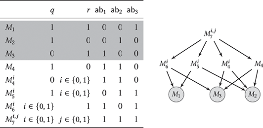
Figure 12 The order  on the models of Example 21. Highlighted are the
  -minimal models. The atoms
  and
and  are true in every model of
  .
.
Figure 12Long description
The row-wise data is as follows: Row 1 (highlighted): M subscript 1: 1, 1, 0, 0 and 1. Row 2 (highlighted): M subscript 2: 1, 0, 0, 1 and 0. Row 3 (highlighted): M subscript 3: 0, 1, 1, 0 and 0. Row 4: M subscript 4: 1, 0, 1,1 and 0. Row 5: M superscript i end superscript subscript 4: 0, i is an element of left curly bracket 0, 1 right curly bracket, 1, 1 and 0. Row 5: M superscript i end superscript subscript 5: 1, i is an element of left curly bracket 0, 1 right curly bracket, 0, 1 and 1. Row 6: M superscript i end superscript subscript 6: i is an element of left curly bracket 0, 1 right curly bracket, 1, 1, 0 and 1. Row 7: M superscript i end superscript subscript 7, : i is an element of left curly bracket 0, 1 right curly bracket, : j is an element of left curly bracket 0, 1 right curly bracket, 1, 1 and 1. On the left, it shows the following sequence: M superscript i, j end superscript subscript 7 leads to M superscript i end superscript subscript 6, M superscript i end superscript subscript 5, M superscript i end superscript subscript 4 and M subscript 4. M superscript i end superscript subscript 6 and M superscript i end superscript subscript 5 leads to M subscript 1. M superscript i end superscript subscript 6 leads to M subscript 3. M superscript i end superscript subscript 5 also leads to M subscript 2. M superscript i end superscript subscript 4 leads to both M subscript 3 and M subscript 2. M subscript 4 leads to M subscript 3 and M subscript 2.
Semantic selections have also been used as a model of the closed-world assumption in McCarthy’s circumscription (McCarthy, Reference McCarthy1980).Footnote 31 In our presentation this is realized by letting  be a set of negated atoms.
Example 22. Suppose Anne checks the online menu of the university canteen and finds the information that fries are served and that either pizza or burger is available. Consider the knowledge base  where
where  ,
,  consists of
  , and
, and  . In Fig. 13 we find the
  -ordering of the models of
  . With
  Anne concludes, for instance,
  and
and  . This is in accordance with the closed-world assumption: what is not listed in the menu is assumed not to be offered.

Figure 13 Models of  in Example 22 with highlighted
  -minimal models.
Figure 13Long description
The row-wise data is as follows: Row 1 (highlighted): M subscript 1: 1, 1, 0 and 0. Row 2 (highlighted): M subscript 2: 1, 0, 1 and 0. Row 3: M subscript 3: 1, 1, 1 and 0. Row 4: M subscript 4: 1, 1, 0 and 1. Row 5: M subscript 5: 1, 0, 1 and 1. 6. M subscript 6: 1, 1, 1 and 1. The sequence shows the following: M subscript 6 leads to M subscript 4, M subscript 3 and M subscript 5. M subscript 4 and M subscript 3 further leads to M subscript 1. M subscript 3 and M subscript 5 further leads to M subscript 2.
6 A Roadmap
In this introduction we have explained the main ideas and concepts behind several core methods of NML. In what follows we will deepen our understanding of
the argumentation method in which a reasoner analyzes the interplay between arguments and their counterarguments to determine coherent sets of arguments (Part II);
the methods based on consistent accumulation, temperate and greedy, in which a reasoner gradually commits to more and more defeasible information from the given knowledge base (Part III); and
the semantic method in which a reasoner determines the most normal interpretations of the given knowledge base (Part IV).
We will study metatheoretic properties that come with these methods and discuss central logics from the literature that implement them.
Given that the field of NML comes with such a variety of systems and methods, it will also be our task to provide links between the methods. As we will see, several classes of logics belonging to different methods give rise to the same class of nonmonotonic consequence relations (see Fig. 14 for an overview).

Figure 14 Links between the various methods studied in this Element.
Figure 14Long description
The links are as follows: Semantic Methods is connected to the following: 1. Greedy Accumulation via Thm.16.1; 2. Argumentation via Thm.16.2; 3. Temperate Accumulation via Cor.15.1; Thm.15.2; 4. Fixpoints via Def.16.4. Greedy Accumulation is connected to the following: 1. Argumentation via Prop.12.1; 2. Temperate Accumulation via Rem.1; 3. Fixpoints via Prop.12.1; Thm.10.1. Argumentation leads to the follows: 1. Temperate Accumulation via Thm.11.3; Thm.9.1 and 2. Fixpoints via Def.7.1. Temperate Accumulation is connected to Fixpoints via Thm.10.1.
Part II Formal Argumentation
Argumentation theory as a study of defeasible reasoning has been proposed already by Toulmin (Reference Toulmin1958). His book provides a critique of formal logic as a model of the defeasible nature of commonsense reasoning. While in the early 1980s many NMLs were proposed, we have to wait for the most influential pioneering works in formal argumentation such as Pollock (Reference Pollock1991, Reference Pollock1995) and Dung (Reference Dung1995) until the 1990s. What distinguishes these approaches from earlier NMLs is the prominent status of arguments and defeat. The ambition is to provide both an intuitive and unifying account of defeasible reasoning. Recently, Mercier and Sperber (Reference Mercier and Sperber2017) have made a strong case for the argumentative nature of human reasoning. Together with the rich tradition in informal argumentation theory (e.g., Eemeren & Grootendorst, Reference Eemeren and Grootendorst2004; Walton et al., Reference Walton, Reed and Macagno2008) this strongly motivates formal argumentation as an account of defeasible reasoning which is close to human reasoning practices.
In this part we deepen our understanding of formal argumentation theory. In Section 7 we explain how Dung’s abstract perspective provides a way to select arguments from an argumentation framework. In Section 8, 9, we present two ways of equipping arguments with logical structure.
7 Abstract Argumentation
In formal argumentation the question as to what follows from a given defeasible knowledge base  is answered by means of an argumentative analysis. It is the essential idea behind abstract argumentation (introduced by Dung (Reference Dung1995) that as soon as the arguments induced by
  are generated and collected in the set
  , and as soon as the attacks between them are determined and collected in the relation
  , we can abstract from the concrete content of those arguments, focus on the directed graph given by
  and select arguments simply by means of analyzing this graph.Footnote 32 The latter is called the argumentation framework for
  . The argumentation semantics defined in the following definition offer criteria to select arguments that form a defendable and consistent stance. We call the selected sets of arguments A-extensions of
  . A-extensions form the basis of three types of nonmonotonic consequence relations:
  , and
, and  (see Table 3). Due to its strict division of labor between argument and attack generation, on the one hand, and argument selection with its induced notion of nonmonotonic consequence, on the other hand, formal argumentation offers a transparent and clean methodology.
Definition 7.1 (Argumentation Semantics, Dung (1995)). Let  be an argumentation framework and
  a set of arguments. We say that
  defends
  if for all
  , if
, if  then there is a
  such that
  . We write
  for the set of arguments that are defended by
  . In Table 4 we list several types of A-extensions.

Table 4Long description
The table consists of two columns: X is, and iff. It reads as follows: Row 1: conflict-free; for all a, b elements of X, (a, b) not an element of att. Row 2: admissible; X subset or equal to defended (X). Row 3: complete; X equals defended (X). Row 4: grounded; X is the unique subset or equal to-minimal complete set. Row 5: preferred; X is a subset of or equal to the maximal admissible. Row 6: stable; X is conflict-free and for all a element of Arguments backslash X, there is a b element of X such that (b, a) element of Arguments.
In Fig. 15 we see the logical connections between the different argumentation semantics, all of which have been shown in Dung (Reference Dung1995). Dung also showed that, except for stable extensions, extensions of all other types always exist (they may be empty, though) and the grounded extension consists exactly of those arguments that are contained in every complete extension. Stable extensions often do not exist in frameworks that give rise to odd cycles: consider, for instance, 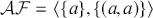 in which neither
  nor
nor  is stable. In Fig. 16 we find an argumentation framework with five arguments. Depicted are some of its extensions.

Figure 15 Relations between argumentation semantics. Every extension of the type left of an arrow is also an extension of the type to its right.

Figure 16 Left: An argumentation framework composed of five arguments. Highlighted in the center and on the right are its two preferred extensions. The extension in the center is the only stable extension. The grounded extension in this example is  .
.
8 ASPIC+
We now move from abstract to structured argumentation.Footnote 33 This means that our arguments will now get a logical form and attacks will be defined in terms of logical relations between arguments. ASPIC+ is one of the most prominent and most expressive frameworks in formal argumentation (Modgil & Prakken, Reference Modgil and Prakken2013). Arguments are generated on the basis of the inference rules and assumptions in a given knowledge base  of the form
  (see Definition 5.1). We let
  denote the set of all arguments induced by
  . In the context of ASPIC+ we frequently find three types of attacks. In order to define them, we need to enhance knowledge bases with two elements. (a) A contrariness relation
  associates formulas with a set of contraries, for example,
  or
or  . (b) A naming function
  allows us to refer to defeasible rules
  in the object language by
  . So our knowledge bases will have the extended form
  .
.
Definition 8.1. Where  , we define three types of attacks:
- Rebut:
- rebuts in iff is of the form and .
- Undercut:
- undercuts in iff is of the form where the top rule is and .
- Undermining:
- undermines in a defeasible assumption in case and .


An informal example of a rebut is one where Peter calls upon weather report 1 to argue that it will rain, while Anne counters by calling upon weather report 2 that predicts the opposite. An undercut may occur in a case of specificity: while Peter argues that Tweety can fly based on the fact that Tweety is a bird and birds usually fly, Anne counters that the default “Birds fly” is not applicable to Tweety since Tweety is a penguin and, as such, Tweety is exceptional to “Birds fly.” Undermining happens if Anne argues against one of Peter’s basic (defeasible) assumptions: Peter may argue that they should go and buy groceries, since the shop is open, when Anne reminds him of the fact that it is a public holiday and therefore shops are closed.
Whenever the defeasible elements of a knowledge base differ in strength, not every attack may be successful. In the context of ASPIC+ we refer to successful attacks as defeats. There are various ways defeats can be defined, but they are all based on a lifting of  to the level of arguments (recall that
  orders the defeasible elements of our knowledge base
  ). We present here the most common approach, called weakest link. To simplify things, we also suppose that
  is a total preorder (so it is reflexive, transitive and total). Where
  , we let
  if there is a
  such that for all
  ,
,  . Then, for two arguments
  , we let
  iff
iff  .Footnote 34 We now say that
  defeats
  iff
iff  attacks
  (Definition 8.1) and (i)
  or (ii) the attack is an undercut.Footnote 35
In the special case in which no preference order  is specified in the knowledge base,
  defeats
  iff
iff  attacks
  . If the naming function is left unspecified in
  , undercuts are omitted.
Definition 8.2. Let  be a knowledge base.
  is an ASPIC+-based argumentation framework, where for
  ,
,  iff
iff  defeats
  .
.
A-extensions obtained via the different argumentation semantics  (grounded, preferred, stable, etc.) in Definition 7.1 can serve as a basis for the three types of consequences, defined exactly as in Definition 5.2 and Table 3 in Section 5.1.
Example 23. We consider the knowledge base  , where
  ,
,  ,
,  ,
,

 , and
, and  . In order to define
  we “rank” the members of
  as indicated in the superscripts of the defaults and let the rank of the defeasible assumption
  be
be  . Where
  , we then let
  iff
iff  .
.
The arguments induced by  and the corresponding argumentation framework are depicted in Fig. 17. We note that
  is defeated by
  despite the fact that
  is weaker than
  (by comparing their weakest links) since the attack is an undercut, for which the strength of the attacker plays no role. The defeat between
  and
and  is symmetric. We have an undermine attack from
  to
to  , while the other way around it is a rebuttal. In Table 5 we list the different argumentation extensions and the corresponding consequence relations.

Figure 17 The argumentation framework for Example 23. Solid arrows represent rebuttals, dashed arrows undermining, and dotted arrows undercuts.

Table 5Long description
The table has four columns: Complete, Grounded, Preferred, and Stable. It reads as follows: Row 1: X subscript zero equals set of a subscript zero, b subscript one; X subscript zero; blank; blank. Row 2: X subscript one equals set of a subscript zero, b subscript one, b subscript two, b subscript three; blank; X subscript one; blank. Row 3: X subscript two equals set of a subscript zero, b subscript one, c subscript zero, c subscript one, c subscript two, c subscript three; blank; X subscript two; X subscript two. Row 4: Turnstile intersection P-extension: set of p and s; set of p and s; set of p, s, and u; set of p, q, u, s, t, and v. Row 5: Turnstile intersection A-extension: set of p and s; set of p and s; set of p and s; set of p, q, u, s, t, and v. Row 6: Turnstile union extension: S equals set of p, q, not q, t, s, not s, u, and v; set of p and s; S; set of p, q, u, s, t, and v.
Example 24. Consider the knowledge base  (without preferences), where
  and
and  . We have, for instance, the following arguments:

Table 05Long description
The six knowledge base rules are: 1. a subscript 1 equals p implies q; 2. a subscript 2 equals p implies s; 3. a subscript 3 equals p implies not (q and s); 4. a subscript 4 equals a subscript 1, a subscript 2 right arrow q and s; 5. a subscript 5 equals a subscript 1, a subscript 3 right arrow not s; and 6. a subscript 6 equals a subscript 2, a subscript 3 right arrow not q.
The reader may be puzzled by on odd restriction in Definition 8.1, namely, when attacking an argument in which inference rules have been applied, only attacks in the heads of defeasible rules are allowed. Why did we not simply define:  attacks
  iff
iff  ? Figure 18 features the resulting argumentation framework. We observe that there is now a preferred (and stable) extension with the conclusions
  and
and  . This may be considered as unwanted if we want our A-extensions to represent rational and therefore consistent stances of debaters.

Figure 18 Example 24 with the inconsistent preferred and stable extension  .
.
Problems such as the one highlighted in our previous example show the need for a set of design desiderata, or rationality postulates, that argumentation-based NMLs should fulfill. The following have become standard in the literature (Caminada & Amgoud, Reference Caminada and Amgoud2007). Given a standard of consistency, a knowledge base  , an argumentation semantics, an A-extension
  based on it, and the argumentation framework
  , we define
- Direct consistency.
For all
, is consistent.- Indirect consistency.
- is consistent.
- Strict closure.
Where
and , also .


In Example 24 we have seen that allowing in our simple framework for “unrestricted” rebut results in a violation of indirect consistency and strict closure,Footnote 36 unlike the unrestricted rebut of Definition 8.1.
Another rationality property has to do with syntactic relevance. We give an example to motivate it.
Example 25. Consider the knowledge base  , where
  ,
,  , and
, and 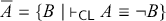 . Clearly, the grounded extension will contain the argument
  and therefore both
  and
and  follow with
  and
and  .
.
We now extend our knowledge base to 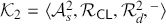 , where
  and
and  . Figure 19 shows a relevant excerpt of the argumentation framework for
  . Argument
  is obtained by the rule
  that holds due to the classical explosion principle.
Note that we only added information to  that is syntactically irrelevant to both
  and
and  . Nevertheless, the grounded extension of
  only consists of arguments that do not involve defeasible rules (such as
  or
or  ). Therefore,
  is not part of it. As a consequence,
  and
and  will deliver only classical consequences of
  , but not anymore
  .
.

Figure 19 Excerpt of the argumentation framework of Example 25.
The rationality property noninterference (Caminada et al., Reference Caminada, Carnielli and Dunne2012) expresses, informally, that adding syntactically irrelevant information to a knowledge base should not lead to the loss of consequences. Our example shows that this property does not hold for grounded extensions.
9 Logic-Based Argumentation
Another line of research within structured argumentation is logic-based (or deductive) argumentation. In what follows we will show that it has close connections to temperate accumulation and that, just as in the case of ASPIC+, ill-conceived combinations of attack forms and argumentation semantics can lead to undesired metatheoretic behavior.
Logic-based argumentation has been proposed, for instance, in Arieli and Straßer (Reference Arieli and Straßer2015) and Besnard and Hunter (Reference Besnard and Hunter2001). Our presentation follows the approach in Arieli et al. (Reference Arieli, Borg and Straßer2023), but simplifies it in some respects.Footnote 37 Knowledge bases have the form  , where the set of strict rules
  is induced by an underlying Tarski logic
  .
.
In Definition 5.1, arguments are proof trees. In the context of knowledge bases without defeasible rules and for which the strict rules are induced by a base logic  , arguments are often modeled more abstractly simply as premise-conclusion pairs.
Definition 9.1. Where  , we let
  . Where
  is an argument in
  ,
,  and
and  . Where
  ,
,  .
.
Attacks between arguments can be defined in various ways. Some examples are given in Table 6.Footnote 38

Table 6Long description
The table consists of four columns: Type, Attacker, Attacked, and Conditions. Row 1: Defeat; A subscript 1, not A subscript 2; A subscript 2 union A prime subscript 2, C; A subscript 2 not equal to the empty set, A subscript 2 is a subset of A subscript d. Row 2: DirDefeat; A subscript 1, not A; A subscript 2 union the set containing A, C; A is an element of A subscript d. Row 3: ConDefeat; A subscript 1, not A subscript 2 back slash A subscript s; A subscript two, C; A subscript 1 is a subset of A subscript s, A subscript 2 intersection A subscript d is not equal to the empty set.
Definition 9.2. Let  be a nonempty set of attack types based on the knowledge base
  from Table 6, arguments be defined as in Definition 9.1, and
  be defined by
  iff
iff  attacks
  in view of an attack type in
  . We let
  be the argumentation framework induced by
  and
and  . For a given argumentation semantics
  (see Table 4) and an attack type
  , we denote the corresponding set of A-extensions by
  and the underlying nonmonotonic consequences analogous to Table 3. For instance,
- iff in every -extension there is an argument .


Let in the following  , and
, and  .
.
Example 26. We let  , where
  and
and  . In Fig. 20 we see (a fragment of) the argumentation framework
  . We note that for
  the grounded extension concludes
  , but not for
  . The latter is counterintuitive since
  is syntactically unrelated to the conflicts in
  and
and  and the conflict in
  and
and  . On the right (center and bottom) we see the two stable resp. preferred extensions for this example. In both cases we can conclude
  and the floating conclusion
  .
.
We also note a correspondence between the argumentative extensions and selections based on maxicon sets of  (see Section 5.2.3). We have
  and
and  . So, in our example, the grounded semantics induces the same consequence relations
  and
and  as
as  for
for  , while the stable and preferred semantics (
 ) induce the same consequence relations
  as
as  for any
  (recall Section 5.2.3 and Corollary 5.1). This is not coincidental, as we see with Theorem 9.1.

Figure 20 Example 26. Left: We let  . The black nodes represent the grounded extension. Dashed arrows correspond to those Defeats and ConDefeats that are not DirDefeats, while solid arrows are (also) DirDefeats. Right top: The grounded extension for
  . Right center and bottom: the two stable resp. preferred extensions.
In fact, there is a close relation between logic-based argumentation and reasoning based on temperate accumulation.Footnote 39
Theorem 9.1 (Arieli et al., 2021b). Let  be a knowledge base. We have:
1.
and , for and .2.
and , for and .


While Theorem 9.1 identifies well-behaved combinations of attack types and argumentation semantics, the following two examples show that one has to be careful in order to avoid counter-intuitive behavior. (Recall similar problems in the context of ASPIC+ in Section 8.)
Example 27. We consider the knowledge base

In Fig. 21 we see that with  we obtain a problematic stable and preferred extension
  featuring the inconsistent set of conclusions
  violating the indirect consistency property (see Section 8). On the right we find the argumentation framework with
  where
where  is not anymore preferred (and therefore also not stable).

Figure 21 Example 27. Left:  . Right:
  .
.
Selected Further Readings
An excellent overview on the state of the art in formal argumentation is provided by the handbook series Handbook of Formal Argumentation (Baroni et al. Reference Baroni, Gabbay and Giacomin2018) and Handbook of Formal Argumentation (Gabbay et al. Reference Gabbay, Giacomin, Guillermo and Thimm2021). Volume 5 of Argument & Computation contains several tutorials on central approaches, such as Modgil and Prakken (Reference Modgil and Prakken2014), and Toni (Reference Toni2014).
Already in the seminal Dung (Reference Dung1995) several embeddings of NMLs in abstract argumentation were provided, including default logic. A recent overview on structured argumentation can be found in Arieli et al., (Reference Arieli, Borg, Heyninck and Straßer2021a). Links to default logic with a special emphasis on preferences are established in, for example, Liao et al. (Reference Liao, Oren, van der Torre and Villata2018); Straßer and Pardo (Reference Straßer, Pardo, Liu, Marra, Portner and Van de Putte2021), and Young et al. (Reference Young, Modgil and Rodrigues2016), connections to maxicon sets are numerous (Arieli et al., Reference Arieli, Borg and Heyninck2019; Cayrol, Reference Cayrol1995; Heyninck & Straßer, Reference Heyninck and Straßer2021b; Reference Vesic2013), and links to adaptive logics are to be found in Borg (Reference Borg2020), Heyninck and Straßer (Reference Heyninck, Straßer, Kern-Isberner and Wassermann2016), and Straßer and Seselja (Reference Straßer and Seselja2010), and to logic programming in Caminada and Schulz (Reference Caminada and Schulz2017); Heyninck and Arieli (Reference Heyninck and Arieli2019), and Schulz and Toni (Reference Schulz and Toni2016). Nonmonotonic reasoning properties of several systems of structured argumentation are studied in Borg and Straßer (Reference Borg, Straßer and Lang2018; Reference Čyras, Toni, Black and Modgil2015; Čyras and Toni (Reference Heyninck and Straßer2021a), and Li et al. (Reference Li, Oren and Parsons2018). Probabilistic approaches can be found, for instance, in Haenni (Reference Haenni2009); Hunter and Thimm (Reference Hunter and Thimm2017), and Straßer and Michajlova (Reference Straßer and Michajlova2023). The Handbook of Formal Argumentation offers an excellent overview and detailed surveys of central topics in the area (see Handbook of Formal Argumentation, Reference Gabbay, Giacomin, Guillermo and Thimm2021).
Part III Consistently Accumulating Defeasible Information
10 Consistent Accumulation: General Setting
In this section we study in a systematic way the two variants of the consistent accumulation method: greedy and temperate accumulation. First, in Section 10.1 we present the algorithms GreedyAcc and TemAcc in the settings of knowledge bases in the general form of Section 4 (including preferences). Then, in Section 10.2 we present alternative characterizations in terms of fixed points. In Section 10.3 we study metatheoretic properties of extensions and nonmonotonic consequences. While this section provides a general perspective, we dive into particularities and concrete systems in Sections 11 and 12.
10.1 Greedy and Temperate Accumulation
We now consider knowledge bases with all components

as introduced in Section 4, with the only restriction that the set of defeasible elements in  ,
,  , is finite. As compared to Part I, we slightly generalize our two accumulation methods, greedy and temperate accumulation, by taking into account preferences among elements in
  . For this, we suppose there to be a reflexive and transitive order
  on
on  .
.
In the following we suppose for any given  a formal language
  , a class of associated knowledge bases
  , a notion of what it means that a set of sentences
  is (in)consistent, for each
  a set
a set  of arguments based on
  , and for each
  a notion
  of conclusion and
  of the defeasible part of
  (e.g., Definitions 5.1, 9.1 and 11.3). Moreover, where
  ,
,  . Many of the results presented in this part of the Element (e.g., the metatheoretic insights in Section 10.3, 11.1) will not rely on a specific underlying notion of argument, but apply to many concrete logics from the literature (such as the ones presented in Section 11.3.1, 11.3.2).
We first discuss greedy accumulation. As explained in Section 5.2, the main idea behind the algorithm is to build a D-extension by accumulating (1) triggered and (2) consistent defeasible information  . Since we now consider prioritized defeasible information, we add the requirement (3) that
  is
is  -maximal with properties (1) and (2). Let us make this precise.
Definition 10.1. For a defeasible rule  , we let
  and
and  . Similarly, for any
  , we let
  and
and  . Then, where
  and
and  , we say that
- is triggered by iff .Footnote 40
- is consistent with iff is consistent.
- iff and for all , .


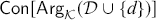


We write  for all the elements in
  that are consistent with
  ,
,  for all elements in
  triggered by
  , and
, and  for all the elements in
  that are triggered by
  .
.
Note that our definition implies that defeasible assumptions are automatically triggered. Algorithm GreedyAcc generates D-extensions for the greedy accumulation method. The A- resp. the P-extension associated with a D-extension  is defined by
  resp. by
  . We write
  resp.
resp.  for the set of A-resp. P-extensions for
  . In this way we obtain the consequence relations
  and
and  (see Table 3), where the superscript indicates that the underlying extensions have been obtained via greedy accumulation.
Example 28 (The order puzzle, Example 11 cont.). We recall the knowledge base  containing the preference order:
  (supposing reflexivity and transitivity). Our algorithm GreedyAcc has exactly one run in which in the first round of the loop
  is added to
  , since it is the
  -preferred one among the two triggered and consistent defaults
  and
and  . In the second round only
  is triggered and consistent. So we end up with
  and GreedyAcc terminates since the remaining default
  is inconsistent with the set of the already selected ones. This implies that
  for all
  .
.

Algorithm 3Long description
The Algorithm displays in eight lines: 1. procedure Greedy accumulation (K), where K equals (A subscript s, A subscript d, R subscript s, R subscript d, R subscript m, subset or equal). 2. Defeasible asterisk left arrow empty set, init D-extension. 3. while Trig subscript K superscript T (Defeasible asterisk) backslash Defeasible asterisk not equals empty set do. 4. (nondeterministically) choose d element of max subscript subset or equal to (Trig subscript K superscript T (Defeasible asterisk) backslash Defeasible asterisk). Defeasible asterisk left arrow Defeasible asterisk union the set containing d, update D-extension. 6. end while, no more triggered and consistent defaults. 7. return Defeasible asterisk, return D-extension. 8. end procedure.
We now move to temperate accumulation which is characterized by the algorithm TemAcc. Recall that the main difference from greedy accumulation is that, when building D-extensions, temperate accumulation also considers nontriggered defaults that are consistent with the already accumulated defeasible elements. The set of D-, A-, and P-extension of  (denoted by
  ,
,  , and
, and  ) and the consequence relations
  , and
, and  are defined in analogy to the greedy case.

Algorithm 4Long description
The Algorithm displays code in eight lines: 1. procedure Temperate accumulation(K), where K equals (A subscript s, A subscript d, R subscript s, R subscript d, R subscript m, subset or equal). 2. Defeasible asterisk left arrow empty set, init D-extension. 3. while Cons subscript K superscript T (Defeasible asterisk) backslash Defeasible asterisk not equals empty set do. 4. (nondeterministically) choose d element of maximum subscript subset or equal to (Cons subscript K (Defeasible asterisk) backslash Defeasible asterisk). 5. Defeasible asterisk left arrow Defeasible asterisk union {d}, update D-extension. 6. end while, no more consistent defaults. 7. return Defeasible asterisk, return D-extension. 8. end procedure.
Example 29 (Example 28 cont.). We now apply TemAcc to  . There is again only one possible run: in the first round we choose (the nontriggered)
  as it is preferred over the other two defaults. In the second round we choose
  as it is preferred over
  . This is when TemAcc terminates since the only remaining default
  is not consistent with
  . This implies that
  for all
  .
.
This shows that unlike in the nonprioritized setting, for knowledge bases with preferences there may be D-extensions for temperate accumulation that do not correspond to D-extensions for greedy accumulation.
10.2 Accumulation and Fixed Points
In this section we consider alternative characterizations of our two accumulation methods. Instead of using iterative algorithms such as TemAcc and GreedyAcc, we now describe these reasoning styles, that is, the D-extension they characterize, as fixed points of specific operations  . The underlying idea is that the possible final products of the reasoning process of a rational agent can be characterized as equilibrium states based on the given knowledge base
  . In what follows, we only consider knowledge bases without preferences.
Lemma 10.1. Let  be a knowledge base. Then,
  iff
iff  .
.
Proof. Let  . By Definition 5.3 (i) and Definition 10.1,
  . If
. If  , then
  by Definition 5.3 (ii), and so
  . The other direction is similar. □
Theorem 10.1. Let  be a knowledge base and
  .
.
1.
is a D-extension generated by TemAcc iff .2.
is a D-extension generated by GreedyAcc iff .


Proof. Item 1 follows with Proposition 5.1 and Lemma 10.1.
Consider Item 2. ( ) Let
) Let  be produced by GreedyAcc such that
  in round
  and
and  for
for  .
.
“ ”. Let
  . So
. So  for some
  . We have to show that
  . Since
  ,
,  . Assume for a contradiction that
  . So, there is a
  -minimal
  such that
  is inconsistent in
  . Let
. Let  be the element in
  with maximal index. If
  ,
,  . If
. If  ,
,  . Each case is a contradiction. So,
  and so
  .
.
“ ”. Let
  . By the guard of the while-loop (line 3),
  .
.
( ) Let now
  . It can easily be seen that
  can be enumerated by
  in such a way that
  ,
,  ,
,  , and
, and  and
and  . Moreover, there is a run of GreedyAcc in which each
  is added to the scenario at round
  for each
  . Note that the algorithm terminates after round
  since
since  . □
. □
An advantage of the characterization of D-extensions in terms of fixed points as in Theorem 10.1 or with maxicon-sets as in Proposition 5.1 is that the restriction to finite sets of defeasible information  in our knowledge bases can be lifted. The restriction was necessary to warrant the termination of GreedyAcc and TemAcc.
10.3 More on Nonmonotonic Reasoning Properties
In this section we take another, more detailed look at abstract properties of nonmonotonic consequence relations (see Section 2.2). To simplify things, we will study them in a nonprioritized setting.
10.3.1 Knowledge Bases and Abstract Properties of Consequence Relations
Now that we have a better understanding of knowledge bases, let us have another look at the properties introduced in Section 2.2. Recall that consequence relations are used to study the question of what follows from a given defeasible knowledge base. An  gives an answer to this question on the basis of the coherent units of information provided by its underlying model of knowledge representation.Footnote 41 It gives rise to nonmonotonic consequence relations
  that hold between knowledge bases (in its associated class
  ) and sentences in its object language
  . In proof-theoretic approaches consequences will be determined by the given extensions of the knowledge base, while in semantic approach they will be based on (typically a selection of) its models.
In the remainder of the Element it will be our task to explain different central methods of knowledge representation and consequence underlying NMLs. Before doing so, we have to comment on what the introduction of knowledge bases means for the abstract study of nonmonotonic consequence presented in Section 2.2. There, the left-hand side of  merely consisted of sets of sentences, but defeasible knowledge bases typically come with more structure. That means that the reasoning principles discussed in Section 2.2 need to be disambiguated. For example, one may distinguish between a strict and a defeasible form of cautious (or rational) monotonicity (see Fig. 22). Where
- ,
- ,


Figure 22 Versions of cautious monotonicity with defeasible knowledge bases
Figure 22Long description
Conclusions lead to strict A subscript s via C M subscript s. Conclusions lead to defeasible A subscript d via C M subscript d. Inference engine loops back to inference engine via meta R subscript m.
and where  , we define:

Table 06Long description
The list is as follows: 1. CM subscript i (turnstile): K turnstile A and K turnstile B implies K oplus subscript i B turnstile A. 2. CT subscript i (turnstile): K turnstile A and K oplus subscript i B turnstile A implies K turnstile B. 3. C subscript i (turnstile): CM subscript i (turnstile) and CT subscript i (turnstile) hold. 4. M subscript i (turnstile): K turnstile A implies K oplus subscript i B turnstile A. 5. OR subscript i (turnstile): K oplus subscript i A turnstile C and K oplus subscript i B turnstile C implies K oplus subscript i (A or B) turnstile C. 6. LLE subscript i (turnstile): A element of Cn subscript R subscript s of set of B, B element of Cn subscript R subscript s of set of A, and K oplus subscript i A turnstile C implies K oplus subscript i B turnstile C. 7. Ref (turnstile): K oplus subscript s A turnstile A. 8. RW (turnstile): K turnstile A and B element of Cn subscript R subscript s of set of A implies K turnstile B.
Since it seems not desirable to expect for defeasible assumptions to be derivable in just any given context, we didn’t include reflexivity under the addition of defeasible assumptions ( ). Similarly, we only stated the RW and LLE in the less demanding version relative to strict rules (as opposed to defeasible rules).
Definition 10.2. Let  . A nonmonotonic consequence relation
  is
is  -cumulative if it satisfies RW
  , LLE
, LLE  , Ref(
 ), and C
  . It is
  -preferential if it additionally satisfies OR
  .
.
10.3.2 Nonmonotonic Reasoning Properties and Extensions
So far, we have discussed cumulativity and related properties in the context of nonmonotonic consequence relations. We now consider these and similar properties from the perspective of extensions. The shift in perspective is well-motivated since, after all, nonmonotonic consequence is determined by the given extensions (see Table 3). In view of this, nonmonotonic reasoning properties should have counterparts from a perspective more focused on knowledge representation. E.g., where cautious monotonicity and transitivity concern the robustness of the consequence set under the addition of consequences to the knowledge base, we should expect a similar robustness of the set of extensions.
In this section we show that many metatheoretic properties hold for both accumulation methods if the underlying notion of argument satisfies some basic requirements.
Given a knowledge base  , a sentence
  , and a set
  , we let
  ,
,  ,
,  , and
, and

Definition 10.3. Let  be an NML based on consistent accumulation with an associated class of knowledge bases
  and let
  . We define the following properties for
  . For all
  and all sentences
  , if
, if  , then
CM
(PExt) holds, if implies .CM
(DExt) holds, if implies .CT
(PExt) holds, if implies .CT
(DExt) holds, if implies .


Moreover,
C
(PExt) holds, if CT (PExt) and CM (PExt) hold.C
(DExt) holds, if CT (DExt) and CM (DExt) hold.


These notions are related as in Fig. 23 (see Theorem 10.2) for D-extensions induced by greedy or temperate accumulation and for any underlying notion of argument, as long as it fulfills the following requirements.

Figure 23 Relations between extensional and consequence-based notions of cumulativity, cautious transitivity and monotonicity (where  ).
).
(arg-trans) Let  and
and  . If there is an
  with
with  , then for all
  , there is a
  with
with  .
.
The criterion states that adding a conclusion  to
to  and
and  does not generate new conclusions:
  .
.
(arg-mono) Let  and
and  . We have
  .
.
The criterion expresses that adding assumptions to a knowledge base does not result in the loss of arguments.
(arg) (arg-trans) and (arg-mono).
Since by the definition of  , we have
  for any
  , by (arg-mono),
  . Therefore, if (arg) holds and
  , then
  .
.
Lemma 10.2. Definitions 5.1 and 9.1 satisfy (arg).
Proof. In the case of Definition 9.1 this follows by the monotonicity and the transitivity of  . (arg-mono) follows directly by Definition 5.1. For (arg-trans), let
  , where
  for some
  . Let
. Let  be the result of replacing every
  in
in  by
by  . Clearly
  and
and  . □
. □
CT  (DExt) and CM
  (DExt) (highlighted in Fig. 23) have a central place. Instead of showing the corresponding properties CT
  and CT
  for the nonmonotonic consequence relations directly, one can show the corresponding extensional principles.Footnote 42
Theorem⋆ 10.2. Given (arg), the logical dependencies of Fig. 23 hold for both accumulation methods.
Moreover, both accumulation methods satisfy CT  (DExt) if (arg) holds.
Proposition⋆ 10.1. Let  . Given (arg), CT
 (DExt) holds for both accumulation methods.
Also LLE and RW hold given some intuitive requirements on the underlying notion of argument.
(arg-re) Let  . If
. If  and
and  , then for every
  there is a
  with
with 

The criterion expresses that if assumptions in the knowledge base are replaced with equivalent ones, we can still conclude the same sentences.
(arg-strict) For all  , (i)
, (i)  and (ii) for all
  and all
  , if
, if  then
then  .
.
The criterion expresses that every strict assumption gives rise to an argument and arguments can be extended by strict rules.
Lemma 10.3. Definitions 5.1 and 9.1 satisfy (arg-re), and (arg-strict).
Proof. Consider Definition 5.1. (arg-strict) follows trivially. For (arg-re), let  and
and  . So, there is a
  of the form
  . Let
. Let  be the result of replacing each
  in
in  by
by  . Then
  and
and  satisfy the requirements of (arg-re). The proof for Definition 9.1 is similar, making use of the transitivity of
  . □
. □
Proposition⋆ 10.2. Let  ,
,  and
and  . If (arg-re), LLE
 (
( ) holds.
Proposition⋆ 10.3. Let  and
and 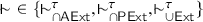 . If (arg-strict), Ref(
 ) and RW(
 ) hold.
11 Temperate Accumulation: Properties and Some Concrete Systems
In this section we study temperate accumulation in more detail. We show that it gives rise to preferential consequence relations (Section 11.1), if some basic conditions are met. Moreover, by “naming” default rules the structure of knowledge bases can be simplified (Section 11.2.1). Temperate accumulation can be characterized in terms of formal argumentation (Section 11.2.2).
Finally, we present two families of systems based on temperate accumulation: reasoning with maxicon-sets (Section 11.3.1) and input–output logics (Section 11.3.2) and apply the results from Section 11.1 to them.
11.1 Cumulativity and Preferentiality
The temperate accumulation method often yields cumulative or even preferential consequence relations. Table 7 gives an overview for the following two classes of knowledge bases:
the “universal” class
containing all knowledge bases of the form ;the class
containing all knowledge bases of the form for a Tarski logic . In this context we suppose that arguments are defined by Definition 9.1 and fulfill the following two properties:(arg-ex) it is explosive in the sense that a set of sentences is inconsistent iff its consequence set is trivial; and
(arg-or)
iff and .Footnote 43

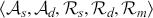


Table 7Long description
The table consists of five columns. The first column lists two knowledge bases: K subscript omega and K subscript A d. The next four columns are grouped under two headers: i-cumulativity and i-preferentiality. Under i-cumulativity: Column 2: Turnstile superscript t e m intersection P-extension. Column 3: Turnstile superscript t e m intersection A-extension. Under i-preferentiality: Column 4: Turnstile superscript t e m intersection P-extension. Column 5: Turnstile superscript t e m intersection A-extension. Row 1: K subscript omega, tick in all four consequence relation columns; each entry references Corollary Eleven point One. Row 2: K subscript A d, tick in the first three consequence relation columns, referencing Corollary Eleven point One; the fourth column also has a tick, referencing Theorem Eleven point One.
As the reader may expect, the results in this section depend also on the underlying notion of argument construction (see Fig. 24 for an overview). In the following we show that any NML based on temperate accumulation and on the argument construction in Definition 5.1 or another definition satisfying (arg-re), (arg-strict), and (arg), satisfies C  (DExt) (for
  ) and is therefore cumulative, that is, C
  (
( ) holds for
  .
.

Figure 24 Nonmonotonic reasoning properties for temperate accumulation, where  ,
,  , and
, and  .
.
Proposition⋆ 11.1.
Let  . Given (arg), C
 (DExt) holds for
  .
.
With Theorem 10.2 and Propositions 10.1 to 10.3 we get:
Corollary 11.1. Let  and
and  . Given (arg), (arg-re), and (arg-strict),
  is
is  -cumulative for
  .
.
In the presence of defeasible rules OR( ) does not hold in general.
Example 30. Let  and
and 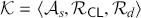 with
with  and
and 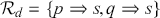 . Clearly,
  while
while  and
and  .
.
There are good news, however, for knowledge bases in  ,
,  is
is  -preferential for
  .
.
Theorem 11.1. Let  .
.  is
is  -preferential for
  .
.
Proof. In view of Corollary 11.1 and Lemmas 10.3 and 10.2 we only have to show OR( ), where
  . Suppose
  and
and  . We show the case
  . Suppose
  and hence, by Theorem 10.1,
 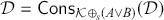 . If
. If  is inconsistent in
  , then
  by (arg-ex). Else, assume for a contradiction that there is a
  for which
  that is consistent in
  . So,
. So,  is nontrivial and by (arg-or) so is
  . So
. So  which is a contradiction. So,
 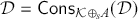 and hence, by Theorem 10.1,
  . Thus,
  since
since  . So, in any case
  .
.
For an analogous reason  . By (arg-or),
  . Hence,
  . □
. □
The preceding result does not consider  . We will show in Section 11.3.1 that OR(
 ) does not hold even for
  .
.
As a last result in this section we show that  is monotonic.
Proposition 11.2.  (and so also CM
 and RM
 ) hold for
  .
.
Proof. Let  and suppose
  . Thus, there is a
  for which there is an
  with
with  . We have to show that
  where
where  is an arbitrary sentence. We have,
  . So,
. So,  is consistent in
  . Thus, there is a maxicon-set
  for which
  . We have
  . Thus,
  . □
. □
11.2 Alternative Characterizations
In this section we present two alternative characterizations of temperate accumulation. First, in Section 11.2.1 we show that in temperate accumulation defeasible rules are dispensable in that a given knowledge base featuring defeasible rules can be translated into one without, in such a way that extensions and consequences are preserved. In Section 11.2.2 we show that temperate accumulation can be translated into formal argumentation.
11.2.1 Naming Defaults in Temperate Accumulation
We now show that, in the context of NMLs based on temperate accumulation, every knowledge base of the form  can be translated into a knowledge base of the form
  , which gives rise to the same D- and P-extensions (Theorem 11.2). The idea is to refer (or “name”) the defaults in
  in the object language, add a strict modus ponens–like rule, and a rule that expresses that a default is defeated in case its antecedents hold but its conclusion is false. This implies that genuinely defeasible rules can be “simulated” by strict rules in systems of temperate accumulation.
Suppose in the following that  is a NML based on a language
  with a class of associated knowledge bases
  of the form of
  . We assume that the notion of inconsistency underlying
  satisfies for any set of sentences
  the sufficient condition:
  implies that
  is inconsistent. Our translated knowledge bases
  make use of an enriched language: every sentence in
  is a sentence in
  , for every
  ,
,  and
and  are sentences in
  , nothing else is a sentence in
  . Note that
  is an object-level symbol in
  but not in
  . We write
  [resp.
  ] for the set of all sentences in
  [resp. in
  ].
].
Definition 11.1. Let the translation of a knowledge base  to
to  be given by:

Note that  .
.
Example 31. Recall the knowledge base from Example 9,  with
with  ,
,  ,
,  and
and  . We translate it to
  with
with
- and
- .


Theorem⋆ 11.2. Let  be based on temperate accumulation, let
  be of the form
  , and let
  be the translation defined in Definition 11.1. Then,
  and
and  .
.
11.2.2 Temperate Accumulation as a Form of Argumentation
In the following we give an elegant argumentative characterization of NMLs based on temperate accumulation and on knowledge bases of the type  .Footnote 44 We work under the assumption that (a)
  and
and  are defined as in Definition 5.1 and (b) the inconsistency of a set of defeasible assumptions
  can be argumentatively expressed by
- (⋆)
- is inconsistent in iff for every there is an that concludes that the assumption is false, that is, .


(⋆) holds if  or, more generally, if
  for some logic
  which has the property that
  is inconsistent in
  iff for all
  ,
,  .
.
Definition 11.2. We define the argumentation framework  where
where  for
for  iff
iff  for some
  . Where
  , we let, moreover,
  be the consequence relation induced by the X-extensions and the stable argumentation semantics (see Definition 5.2) and
  be the set of stable A-extensions of
  .
.
Example 32. We consider  . An excerpt from the argumentation framework
  is illustrated in Fig. 25. We note that
  and
and  .
.
We have, on the one hand, two D-extensions according to temperate accumulation,  and
and  , with the corresponding A-extensions
  and
and  and the P-extensions
  and
and  . On the other hand, we have two stable A-extensions of
  (highlighted in Fig. 25), namely
  and
and  , with the corresponding P-extensions
  and
and  .
.

Figure 25 The argumentation framework for the knowledge base of Example 32 based on the arguments to the right. The rectangular node represents a class of arguments based on the inconsistent assumption set  . An outgoing [resp. ingoing] arrow symbolizes an attack from [resp. to] some argument in the class.
The following theorem shows that the observed correspondences are not coincidental.
Theorem 11.2. Let  be an NML based on temperate accumulation for which (⋆) holds and
  be a knowledge base.
1. If
then .2. If
, there is a such that .


Proof. For Item 1 suppose  . By Proposition 5.1,
  . Consider
  such that
  and
and  . By (⋆) and the consistency of
  in
in  ,
,  . Thus,
  is conflict-free.
Let now  . So, there is an
  . Since
  ,
,  is inconsistent in
  and by (⋆) there is a
  with
with  . Thus,
  .
.
For Item 2 let  and
and 
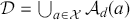 . Clearly,
 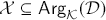 . Assume for a contradiction that there is an
  . By stability, there is a
  such that
  and so
  for some
  . Since
  and
and  , there is a
  for which
  and so
  in contradiction to the conflict-freeness of
  . Thus,
  .
.
By Proposition 5.1, we have to show that  . In view of (⋆) and the conflict-freeness of
  ,
,  is consistent in
  . Suppose
  is such that
  is consistent. If
  , then
 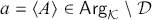 and by stability, there is a
  such that
  and therefore
  . But then, by (⋆),
  is inconsistent in
  . So,
. So,  and therefore
  . □
. □
11.3 Two Families of NMLs from the Literature
In this section we will introduce two well-known families of NMLs, both based on the idea of forming maxicon sets of defeasible information from the given knowledge base.
11.3.1 Reasoning with Maxicon Sets of Sentences
A time-honored family of NMLs has been proposed by Rescher and Manor (Reference Rescher and Manor1970). These NMLs model reasoning scenarios in which an agent is confronted with reliable but not infallible information (e.g., resulting from testimonies, weather reports, and so on) that may give rise to contradictions. Such information is encoded by sets of defeasible assumptions. Clearly, due to the possibility of logical explosion, classical logic cannot be applied to such sets, at least not naively. The basic idea behind Rescher’s and Manor’s approach is to form ( -maximal) consistent sets of defeasible assumptions and reason on their basis. In our terminology these maxicon sets of defeasible assumptions form D-extensions and their classical closures are P-extensions induced by temperate accumulation. We obtain the three types of consequences that have been introduced in Definition 5.2.
While Rescher and Manor considered knowledge bases of the form  , Makinson’s system of Default Assumptions (Makinson (Reference Makinson2005)) also considered strict assumptions and so generalized the considered class of knowledge bases to those of the form
  .Footnote 45 Of course, one may consider other Tarski-logics
  instead of classical logic. Let the class
  consist of all knowledge bases of the form
  . We let:Footnote 46
1.
iff for every .2.
iff there is a for which .3.
iff there is a such that .


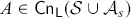


In what follows we let arguments be defined as in Definition 9.1.
Example 33. Consider the knowledge base  where
where  and
and  . We have
  where
where  , and
, and  . Note that the defeasible assumption
  conflicts with the strict assumption
  .
.
We first observe that  is a floating conclusion in view of the conflicting arguments
  and
and  . Indeed,
  while
while  .
.
In view of Proposition 5.1 the three consequence relations  , and
, and  are identical to
  , and
, and  on the class
  . Therefore, the results from Section 11.1 are applicable (Table 8).

Table 8Long description
The table consists of eleven columns. The first column lists three consequence relation types: turnstile subscript m c o n intersection P-extension, turnstile subscript m c o n intersection A-extension, and turnstile subscript m c o n union extension. The next ten columns are titled: M subscript d, M subscript s, C M subscript d, C M subscript s, C T subscript d, C T subscript s, R M subscript d, R M subscript s, O R subscript d, and O R subscript s. Row 1: Turnstile subscript m c o n intersection P-extension: tick in columns C M subscript d, C M subscript s, C T subscript d, C T subscript s, O R subscript d, and O R subscript s. Row 2: Turnstile subscript m c o n intersection A-extension: tick in columns C M subscript d, C M subscript s, C T subscript d, C T subscript s, and O R subscript s. Row 3: Turnstile subscript m c o n union extension: tick in columns M subscript d, M subscript s, R M subscript d, and R M subscript s.
Proposition 11.3. Let  . Then, (i)
  iff
iff  , (ii)
  iff
iff  , and (iii)
  iff
iff  .
.
Proof. We show case (ii). The others are analogous and left to the reader.  , iff, there is an
  with
with  , iff,
  , iff [by Proposition 5.1],
  , iff,
  . □
. □
In view of Corollary 11.1, Theorem 11.1 and Lemmas 10.2 and 10.3 we therefore get:
Corollary 11.2. Let  .
.  is
is  -cumulative. If (arg-ex) and (arg-or) hold,
  is
is  -preferential.
Example 34. Where  , in Table 9 we list counter-examples to (OR) and therefore to the
  -preferentiality of
  and
and  . In Table 10 we find counterexamples to RM
  for
for  .
.

Table 9Long description
The table consists of four columns: K asterisk equals, K Oplus subscript i p, K Oplus subscript i q, and K Oplus subscript i (p or q). It read as follows: Row 1: i equals s, K equals K subscript 1: maxcon (K asterisk); {not q and r}; {not p and r}; {not q and r}, {not p and r}. Row 2: i equals s, K equals K subscript 1: intersection D-extension (K asterisk); {not q not r}; {not p not r}; empty set. Row 3: i equals s, K equals K subscript 1: K asterisk turnstile superscript mcon subscript A-extension r question mark; checkmark; checkmark; cross. Row 4: i equals d, K equals K subscript 2: maxcon (K asterisk); A subscript 2 superscript p backslash {not p} and below it A subscript 2; A subscript 2 superscript p backslash {not q} and below it A subscript 2; A subscript 2 superscript p or q backslash {not p} and below it A subscript 2 superscript p or q backslash {not q} and below it A subscript 2. Row 5: i equals d, K equals K subscript 2: intersection D-extension (K asterisk); A subscript 2 backslash {not p}; A subscript 2 backslash {not q}; A subscript 2 backslash {not p, not q}. Row 6: i equals d, K equals K subscript 2: K asterisk turnstile superscript mcon subscript A-extension r question mark; checkmark; checkmark; cross. Row 7: i is an element of {s, d}, K equals K subscript 3: maxcon (K asterisk); A subscript 3 superscript u Oplus subscript i p and below it A subscript 3 superscript not u Oplus subscript i p; A subscript 3 superscript u Oplus subscript i q and below it A subscript 3 superscript not u Oplus subscript i q; A subscript 3 superscript u Oplus subscript i (p or q) and below it A subscript 3 superscript not u Oplus subscript i (p or q). Row 8: i is an element of {s, d}, K equals K subscript 3: K asterisk turnstile superscript mcon subscript U-extension r question mark; checkmark; checkmark; cross.

Table 10Long description
The table consists of four columns: K asterisk equals, K, K oplus subscript s not (p and r), and K oplus subscript d not (p and r). It reads as follows: Row 1: maxcon of K asterisk; set of p, q and r; set of not p, q and r; set of p; set of not p, q and r; set of p, not (p and r); set of p, q and r; set of not p, q and r, not (p and r). Row 2: intersection D-extension of K asterisk; set of q and r; empty set; empty set. Row 3: K asterisk turnstile superscript m c o n subscript intersection A-extension r question mark; tick; cross; cross. Row 4: K asterisk not turnstile superscript m c o n subscript intersection A-extension not (p and r) question mark; tick; blank; blank. Row 5: K asterisk turnstile superscript m c o n subscript intersection P-extension r question mark; tick; cross; cross. Row 6: K asterisk not turnstile superscript m c o n subscript intersection P-extension not (p and r) question mark; tick; blank; blank.
We end this section with two simple counterexamples concerning the cautious monotonicity and transitivity of  and a positive result concerning its rational monotonicity.
Example 35. Let  . We first let
  . Then,
  and
and  , but
, but  . Note for this that
  . This shows that CM
  and M
and M  don’t hold.
Let now  and
and  . We note that
  (since
  ) and
) and  (since
  ). However,
  . This shows that CT
  does not hold.
Proposition 11.4. Let  ,
,  , and
, and  . Then, RM
 holds.
Sketch of the Proof. Suppose  and
and  and let
  . In view of
  every
every  is consistent with
  . It is therefore easy to see that
  iff
iff  and therefore also
  .
.
11.3.2 Reasoning with Consistent Sets of Defaults and Metarules: Input–Output Logic
Input–output logics (in short, IO-logics) have been first presented in Makinson and Van Der Torre (Reference Makinson and Van Der Torre2000) and in a nonmonotonic setting in Reference Makinson and Van Der Torre2001. We work with the class of knowledge bases  of the type
  , where the strict rules are provided by a Tarski base logic
  (such as classical or intuitionistic logic).Footnote 47 Instead of Definitions 5.1, arguments in IO-logic are constructed according to the following “two-phase” definition in which (a) the derivation of information from strict assumptions by the strict rules and (b) the derivation of defeasible rules from strict and defeasible rules by means of metarules are separated. The detachment of argument conclusions is applied to the results of (a) and (b).
Definition 11.3 (Arguments, Consistency, and Consequences in IO-logic). Let  . Where
  ,
,  iff (a)
  and (b)
  . We let
  and
and  .
.
 is consistent in
  iff there is no sentence
  for which
  .
.
We define D-, A-, and P-extensions as usual (see Section 10). Where  , we will write
  for the induced consequence relation (see Definition 5.2) on the class of knowledge bases
  .
.
In IO-logic metarules play a central role. Paradigmatic rules are:

Table 07Long description
The Paradigmatic rules are: 1. Right Weakening (RW); (A right arrow B), (C implies A) turnstile (C implies B). 2. Left Strengthening (LS): (A right arrow C), (C implies B) turnstile (A implies B). 3. Right Conjunction (AND): (A implies B), (A implies C) turnstile (A implies B and C). 4. Cumulative Transitivity (CT): (A implies B), (A and B implies C) turnstile (A implies C). 5. Left Disjunction (OR): (A implies C), (B implies C) turnstile (A or B implies C). 6. Identity (ID): Turnstile A implies A.
Depending on the underlying class of knowledge bases, we have 12 base systems, summarized in Fig. 26.

Figure 26 The basic input–output logics and their associated knowledge bases where  and
and  .
.
Example 36. Let  where
where  ,
,  , and
, and  . We have three maxicon sets for
  :
:  ,
,  , and
, and  . By Proposition 5.1, we know that these correspond to the D-extension generated by TemAcc. We have
  since
since  doesn’t contain an argument for
  .
.
Note that  is not consistent since it contains the argument
  for
for  and
and  for
for  based on the
  -derivation
IO-logics have found applications in deontic logic where the rules in  are interpreted as conditional norms:
  is read as “
 commits us/you/etc. to bring about
  ” (Parent & van der Torre, Reference Parent, van der Torre, Gabbay, Horty, Parent, van der Meyden and van der Torre2013). The right side of the consequence relation
  encodes the obligations derivable from a knowledge base, where the latter represents the information available about the actual situation
  and the given conditional norms
  . In deontic logic, conflicts between norms can occur in various ways, for example, in terms of contrary-to-duty situations.
Example 37. Let  stand for “helping the neighbor,” and
  for “notifying the neighbor” (Chisholm, Reference Chisholm1963). Consider
  ,
,  and
and  . We have three maxicon sets, namely
  ,
,  , and
, and  . One may object to
  being part of the D-extensions since our strict assumptions express that our agent already determined the outcome
  and so
  would not be action-guiding. Moreover, in
  this leads to a pragmatic oddity according to which an agent should help and also not notify the neighbor. To deal with this problem, knowledge bases have been extended with a set of constraints (such as here
  ) on the output in Makinson and Van Der Torre (Reference Makinson and Van Der Torre2001). In order to simplify the presentation, we have omitted constraints in this section.
We will now consider some of the properties studied in Section 10.3. We say that  has a proper conjunction
  iff (a)
  iff
iff  and (b)
  , …,
, …,  implies
  . In the following we assume that
  has a proper conjunction.
Lemma 11.1. An IO-logic whose metarules include LS and CT satisfies (arg-re) and (arg).
Proof. For (arg-trans) consider a  for which there is an
  and suppose
  . Thus, there are proofs
  resp.
resp.  based on the rules in of
  resp. of
  from
from  . Moreover,
  and
and  . So, there are
  for which
  . By the monotonicity of
  and since
  is a proper conjunction,
  and
and  . Consider the following proof based on the metarules
  :
:

Note that  and so
  .
.
The simple proofs of (arg-re) and (arg-mono) are left to the reader. □
By Lemma 11.1, Propositions 10.2 and 11.1, and Theorem 10.2 we get:
Corollary 11.3. Let  . Any IO-logic whose metarules include LS and CT satisfies C
 and LLE
 .
.
In view of Corollary 11.1 the logics  with
with  from Fig. 26 are
  -cumulative, since their notions of argument satisfy (arg-strict).
Lemma 11.2. Any IO-logic  from Fig. 26 satisfies (arg-strict).
Proof. Concerning (i) we note that if  , since
  , also
  . Concerning (ii), where
  , suppose
  and there are
  . So,
. So,  for each
  . So,
. So,  where
where  . By (LS),
  for each
  . By AND,
  where
where  . Since
  and by RW,
  . □
. □
By Corollary 11.1 and Lemmas 11.1 and 11.2 we get:
Corollary 11.4. Let  and
and  .
.  satisfies
  -cumulativity for
  .
.
Example 38.  -cumulativity is not satisfied for
  since Ref does not hold. Consider
  . Clearly, there are maxicon sets including
  in view of which
  , where
  .
.
The situation is different when considering  . Now, the only D-extension is
  and therefore
  since
since  due to the presence of the metarule
  .
.
The following example demonstrates that the OR metarule allows for a form of disjunctive reasoning that is not available in systems without.
Example 39. Let  , where
  and
and  . Note that
  in view of the proof:
  (by OR and LS) and
  by CT. Note also that
  is consistent. Therefore,
  and
and  . The situation is different for weaker logics; for example, if we let
  where
where  and
and  , then
  and so
  and
and  .
.
If OR is available, we get OR  for base logics that satisfy (arg-or) and (arg-ex) (such as
  , see Section 11.1).
Proposition 11.5. Let  and
and  . If (arg-or) and (arg-ex), we have OR
 for
for  .
.
Proof. Let  . Suppose
  and
and  and consider
  . Assume for a contradiction that
  is inconsistent in both
  and
and  . So, there are
  and
and  . By (arg-ex) and LS,
  for some
  . By (arg-or),
  . So, by OR,
  . This shows that
  is inconsistent in
  , which is a contradiction.
So,  or
or  . Without loss of generality, assume the former. Thus, there is a
  for which
  . Assume for a contradiction that
  is inconsistent in
  . So, there are
  . Since
  and by (arg-or), also
  . But then
  is not consistent in
  , which is a contradiction. So,
  is consistent in
  and by the
  -maximally of
  ,
,  . Since
  ,
,  .
.
Altogether this shows that  . □
. □
An immediate consequence of Corollary 11.4 and Proposition 11.5 is:Footnote 48
Corollary 11.5. Let  . If (arg-or) and (arg-ex),
  satisfies
  -preferentiality for
  .
.
12 Greedy Accumulation: Properties and Reiter’s Default Logic
In this section we take a closer look at greedy accumulation. We start by considering some of the properties of nonmonotonic inference for greedy accumulation in Section 12.1. We then investigate Reiter’s more general formulation of default rules in Section 12.2. In Section 12.3 we show that default logic can be considered a form of formal argumentation.
12.1 Properties of Nonmonotonic Reasoning
As we have seen in Section 10.3, some properties of nonmonotonic inference (Propositions 10.1 to 10.3, in particular CT, LLE, Ref, and RW) hold for greedy accumulation. In this section we present some negative results.
Example 40 (Makinson, 2003). We consider the default theory

We get one D-extension, namely  with corresponding P-extension
  and so
  ,
,  ,
,  , and
, and  .
.
When considering  resp.
resp.  the situation changes. We now have the additional D-extension
  resp.
resp.  with the corresponding P-extension
  . Thus, where
  ,
,  and
and  .
.
The example shows that CM does not hold for greedy accumulation. The next example shows that also OR fails (it is analogous to Example 30 for temperate accumulation).
Example 41. Let  ,
,  , and
, and

We note that  and
and  , although
 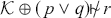 (since the only D-extension of
  is
is  ).
).
It is not surprising that several alternative formulations of default logic have been introduced to obtain CT or OR, a discussion of which goes beyond the scope of this Element (see Section 12.3).
12.2 Nonnormal Defaults
Reiter’s default logic is one of the most prominent NMLs to reason with default rules such as “Birds usually fly.” In Reiter’s original account defaults are more expressive in the sense that they allow one to express additional consistency assumptions. They have the following general form:
 (12.2.1)
Besides the body  and a head
  , each default rule also comes with justifications
  . Where
  is a set of generalized defaults we call knowledge bases of the form
  Reiter default theories.Footnote 49
Example 42. We compare the following two defaults:

Defaults of the form  , for which the justification is identical to the conclusion, are called normal defaults. Both,
  and
and  have the same conditions of defeat: defeat happens if we learn that a person is not guilty or not suspect. However,
  has a weaker conclusion in that it only allows one to infer that the person who has a motive is suspect, but unlike
  it does not warrant the inference to the person’s guilt as well. The use of nonnormal defaults is motivated by cases in which the conclusion is logically weaker than the justification. From the perspective of argumentation these are cases in which we do not only want to retract inferences when being rebutted, but also allow other forms of defeat which are expressed in terms of richer justifications (one may think of these justifications as anchors for undercuts).
Definition 12.1. Let  be a Reiter default theory and
  . We let
  and
and  be defined similar to Definition 5.1:
  iff
iff
- , where . We let , , and .
- , where , , and
We let
, , and .
- , where , , and .
We let
, , and .


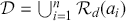


Where  and
and  , we let
  and
and  . We let
  be the set of all
  such that for all
  there is an
  with
with  . Where
  is a set of
  -sentences, we let
  be the set of all
  for which each
  is consistent with
  . We let
  .
.
D-extensions of Reiter default theories are generated by an algorithm, similar to GreedyAcc. However, we need to accommodate the consistency check (in the loop guard, line 3) to the additional ingredient of defaults, their justifications. Since justifications need not be implied by the heads of their respective defaults, the consistency check cannot proceed iteratively anymore. This is to avoid that a justification of a default added earlier conflicts with the head of one added later on in the procedure. Reiter solved this problem by means of a semi-inductive procedure in which the reasoner has to first guess the outcome. Consistency checks are then performed relative to the guessed set of sentences. This results in the algorithm GreedyAccGen.Footnote 50

Algorithm 5Long description
The Algorithm displays code in twelve lines: 1. procedure Generalized Greedy Accumulation (K, D): where K equals A subscript s, R subscript d, R subscript s and D is a subset of R subscript d. 2. D asterisk left arrow empty set: init. 3. E left arrow Con [Arg subscript K (D)]: the guessed P-extension. 4. while exists r in Trig superscript T subscript K (E, D asterisk) backslash D do: scan triggered and consistent defaults. 5. D asterisk left arrow D asterisk union {r}: update scenario. 6. end while: no more triggered and consistent defaults. 7. if D equals D asterisk then. 8. return (D asterisk): correct guess. 9. else. 10. return(failure): incorrect guess. 11. end if. 12. end procedure.
Definition 12.2. A Reiter D-extension of a Reiter default theory  is a set
  for which
  . Its corresponding A-extension is
  , and its corresponding P-extension is
  . We write again
  [resp.
  ,
,  ] for the set of Reiter D- [resp. A-,P-]extensions of
  .
.
Example 43. We consider  , where

We simulate two runs of GreedyAccGen.
1. When running GreedyAccGen
, is the set closed under classical logic. In the first round of the while-loop we add to . In the second round we add since its justification is also consistent with . This leads to failure since .2. We consider GreedyAccGen
. Now is the set closed under classical logic. Since is inconsistent with , the loop terminates with and therefore returns the only D-extension of .


Reiter’s format of defaults and the GreedyAccGen algorithm generalize greedy accumulation as presented in Section 5.2.1. Suppose we have a knowledge base  with only defaults of the form
  . We can translate
  to a Reiter default theory
  by translating each default
  to a Reiter default

Applying GreedyAcc to  and GreedyAccGen to
  will lead to the same D-extensions (under the translation) and therefore the same P-extensions (Łukaszewicz, Reference Łukaszewicz1988).
Nevertheless, the introduction of generalized defaults may lead to scenarios in which no D-extensions exist.
Example 44. Consider  where
where  and
and  only contains the default
  . We have two possible guesses to run GreedyAccGen:
  and
and  . Note that with the first guess the algorithm never enters the while-loop, since the justification
  of
of  is inconsistent with
  and it therefore returns failure. With the second guess, however, since
  is consistent with
  , the while-loop is entered and
  is added to
  , again leading to failure.
Similarly as described in Section 10.2 for normal default theories, also Reiter D-extensions can be characterized in terms of fixed-points.
Proposition⋆ 12.1. Let  be a Reiter default theory,
  , and
, and  .
.  is a Reiter D-extension of
  iff
iff  .
.
12.3 An Argumentative Characterization of Reiter’s Default Logic
In this section we demonstrate that there is a natural argumentative characterization of extensions of Reiter default theories.Footnote 51 For this we use a slightly generalized language  . The unary operator
  will track the consistency assumptions underlying the justifications in generalized defaults. For this, it need not get equipped with logical properties, but it will be used when defining argumentative attacks.
Definition 12.3. Given a Reiter default theory  , we define the argumentation framework
  , where
  ,
,  ,
,  contains
  for every sentence
  , and
, and  ,
,  iff
iff
(12.2.1)
We let  if there is a
  such that
  , where
  for all sentences
  .
.
Example 45 (Ex. 43 cont.). We recall  from Example 43. In Fig. 27 we see an excerpt of
  . The only Reiter D-extension of
  is
is  . Its induced P-extension corresponds exactly to the consequences of the arguments in the only stable A-extension of
  (highlighted).

Figure 27 Illustration of Example 45.
The following result shows that the correspondence between Reiter extensions and stable A-extensions is not coincidental.
Theorem⋆ 12.1 Let  be a general default theory and
  as in Definition 12.3. Then
1. for every Reiter P-extension
of , there is a stable A-extension of for which ,2. for every stable A-extension
of , is a Reiter P-extension of .


Selected Further Readings
Metatheoretic properties of reasoning on the basis of maxicon sets in the style of Rescher and Manor have been thoroughly studied in Benferhat et al. (Reference Benferhat, Dubois and Prade1997). A well-known prioritized version is provided in Brewka (Reference Brewka1989). An overview on the state of the art in input–output logic can be found in Parent and van der Torre (Reference Parent, van der Torre, Gabbay, Horty, Parent, van der Meyden and van der Torre2013). Input–output logics have also been applied to causal and explanatory reasoning in many works by Bochman: Bochman (Reference Bochman2005) is a good starting point. Proof theories for input–output logics that allow for Boolean combinations of defeasible conditionals are presented in Straßer et al. (Reference Straßer, Beirlaen and Van De Putte2016) and van Berkel and Straßer (Reference van Berkel, Straßer, Toni, Polberg, Booth, Caminada and Kido2022). The latter also provides a translation of input/output logic to formal argumentation. Hansen’s approach to (prioritized) deontic conditionals falls within temperate accumulation (Hansen, Reference Hansen2008), while Horty’s follows the greedy approach of deontic logic (Horty, Reference Horty2012).
An overview on many variants of default logic can be found in Antoniou and Wang (Reference Antoniou, Wang, Gabbay and Woods2009). Due to the problems indicated in Section 12.1, some cumulative variants have been proposed (Antonelli, Reference Antonelli1999; Brewka, Reference Brewka1991) as well as disjunctive versions (Gelfond et al., Reference Gelfond, Lifschitz, Przymusinska and Truszczynski1991). In Poole (Reference Poole1985) special attention is paid to specificity.
Moore’s autepistemic logic has close links to default logic (Denecker et al., Reference Denecker, Marek and Truszczynski2011; Konolige, Reference Konolige1988) and to logic programming (Gelfond & Lifschitz, Reference Gelfond and Lifschitz1988). The equi-expressivity of adaptive logics and default assumptions have been shown in Van De Putte (Reference Van De Putte2013). A modal selection semantics (as presented in Sections 5.3 and Section 15) for default logic has been studied in Lin and Shoham (Reference Lin and Shoham1990).
Part IV Semantic Methods
In this final part of the Element we move the focus from syntax to semantics. The main underlying method will be based on imposing preference orders on interpretations and selecting specific interpretations of the given information. In Section 13 we will study a well-known semantics for defaults (Kraus et al., Reference Kraus, Lehman and Magidor1990) based on the idea of preferring more “normal” models over less “normal” ones. In particular, we investigate a sophisticated method to determine the set of defaults that are entailed by a given set of defaults, the Rational Closure (Lehmann & Magidor, Reference Lehmann and Magidor1992). Section 14 provides an overview on some quantitative methods for providing meaning to defaults, including probabilistic methods. In Section 15 we use the idea of ordering models to obtain a semantics for temperate accumulation. Finally, in Section 16 we introduce one of the central paradigms in logic programming, answer set programming, and show how it is closely related to both default logic and formal argumentation. In this way, we once more demonstrate that although the underlying formal methods of NMLs are quite diverse, they often result in the same consequence relations and extensions (recall Fig. 14).
13 A Semantics for Defaults
In Section 1.1 we proposed to interpret defaults  as “If
  then normally/typically/usually/etc.
  ”. The argumentation (Part II) and accumulation methods (Part III) model reasoning with defaults by focusing on inference rules: arguments are formed by treating
  as a defeasible inference rule and the notions of consistency and conflict are used to obtain nonmonotonic consequence relations. In this way the meaning of
  is characterized in a syntax-based, proof-theoretic way.
In what follows, we will interpret  in a semantic, model-theoretic way, by:
- (⋆)
- holds under the most normal/plausible/etc. situations in which holds.


This interpretation naturally leads to nonmonotonicity: while Anne jogs most mornings ( ), rainy mornings are exceptional (
 ).
).
The proposed interpretation can be made precise by using models of the form  with a nonempty set of situations
  which are interpreted by means of an assignment function
  that associates atoms with the set of those situations (also referred to as states) in which they hold, and an order
  that orders situations according to their normality. We read
  (where
  ) as expressing that
  is less normal than
  . Where
  we let
- for an atom iff
- iff
- iff and
- iff or .


We let  be the set of all situations which validate
  and skip the subscript whenever the context disambiguates. Such sets of situations are called propositions. Following the idea expressed in (⋆), we let:Footnote 52
- iff in all , .


Note that validity for  is defined globally, not relative to a given state. In the following we write
  for the set of all
  for which
  , and we write
  in case
  . We will call
  the conditional theory induced by
  .
.
By letting  we can express that
  is “more normal” than
  . Indeed, if in all minimal states of
  ,
,  holds, then the minimal states of
  are
are  -lower than those of
  .
.
One may think of  as a model of the belief state of an agent.
  expresses that if the agent were to learn
  , she would believe
  , where
  means that, absent new information, the agent believes
  . If
. If  , the agent would be less surprised when learning
  than when learning
  .
.
Example 46. Let  where
where  ,
,  ,
,  ,
,  ,
,  , and
, and  . We have, for instance,
  ,
,  ,
,  ,
,  , and
, and  . Thus,
1.
and ,2.
and so ,3. but
and .


In models with infinite sequences of more and more normal states we may face situations in which  is empty, although
  is not. To exclude such scenarios, we restrict the focus on only those models for which it holds that for all sentences
  and all
  there is an
  such that
  . Models that satisfy this requirement are called smooth (Kraus et al., Reference Kraus, Lehman and Magidor1990) or stuttered (Makinson, Reference Makinson2003). In what follows we will discuss some other basic properties one may impose on
  , such as transitivity (if
  and
and  , then also
  ) or irreflexivity (
 ).
).
In particular, we will study two classes of well-behaved models by only considering models for which the underlying order  has specific properties.
13.1 Preferential Models
Let us now state properties one may expect from the conditional theory  induced by a model
  . For this, we adjust the properties from Section 4 to statements of the form
  .
.
The properties are to be read as closure conditions on a set of defaults  . For example, REF states that
  for all sentences
  , or CM states that if
  , then also
  for all sentences
  .
.

Table 08Long description
The list of logical properties includes: 1. Left Logical Equivalence (LLE): If turnstile subscript CL A equivalence B, then A implies C iff B implies C. 2. Right Weakening (RW): If A turnstile subscript CL B and C implies A implies C implies B. 3. Reflexivity (Ref): A implies A. 4. Constructive Dilemma (OR): If A implies C and B implies C, then A or B implies C. 5. Cautious Monotonicity (CM): If A implies B and A implies C, then A and B implies C. 6. Cautious Transitivity (CT); If A implies B and A and B implies C, then A implies C.
We call a set of defaults  preferential theory in case it is closed under these properties.
Given the intuitive nature of the previously mentioned properties, a natural question is: what kinds of models give rise to preferential theories? With Kraus et al. (Reference Kraus, Lehman and Magidor1990) we call  a preferential model in case
  is smooth, irreflexive, and transitive. It is an easy exercise to confirm that the preceding properties hold for
  , where
  is a preferential model. We paradigmatically consider CM (for which smoothness is needed) and OR.
For CM, suppose that  and
and  . In case
  , trivially
  . Otherwise, consider some
  . Assume for a contradiction that
  . Thus, by smoothness, there is a
  such that
  . Since
  and
and  ,
,  and so
  . But then
  was not
  -minimal in
  , a contradiction. So,
  and so
  since
since  . Thus,
  .
.
For OR suppose that  and
and  . If
. If  , trivially
  . Otherwise consider an
  . Assume for a contradiction that
  . Then, there is a
  such that
  . Since
  , this contradicts the
  -minimality of
  . So,
. So,  and so, by the supposition,
  . So,
. So,  .
.
Altogether, it can be shown that:
Theorem 13.1 (Kraus et al., 1990). If  is a preferential model,
  is a preferential theory.
Also the inverse holds, that is, any preferential  can be characterized by a preferential model. As a result, preferential models provide an adequate semantic characterization of preferential theories.
Theorem 13.2 (Kraus et al., 1990). If  is a preferential theory, then there is a preferential model
  for which
  .
.
13.2 Ranked Models
Preferential models do not, in general, validate the rational monotonicity property:Footnote 53
| RM | If  and and  then then  . . |
RM has in  a negative condition. A set of defaults
  is closed under RM if for all sentences
  , if
, if  and
and  , then
  . A preferential theory
  that is closed under RM is called rational.
Example 47 (Example 46 cont.). In our example we have:  and
and  , but
, but  . So,
. So,  does not validate RM, although it is preferential.
As Example 47 shows, preferential models  do not, in general, give rise to rational theories
  . What kind of models are such that their induced conditional theories are rational? The key will be to let all states be comparable.
Preferential models allow for incomparabilities of states in the following sense: there are  for which
  but
but  is not comparable to
  and
and  . We have such a situation in Example 46. We notice that this is responsible for a violation of RM by
  .
.
The RM property holds if the set of minimal states of  is contained in the set of minimal states of
  , in case there are some minimal states of
  that validate
  . In view of
  , one may expect them to be, since there are indeed minimal states of
  that do not satisfy
  and in which therefore
  holds. In our example the outlier is
  . The situation improves if
  is comparable to
  and/or to
  . In the rightmost model of Fig. 28 we have
  ,
,  , and
, and  (while in the model in the center we have
  ).
).

Figure 28 (Left) The preferential model  of Example 46. (Middle and Right) Ranked models
  based on modular extension
  of
of  . The dashed arrow is optional.
A ranked model  is a preferential model for which
  is modular, that is, for all
  , if
, if  , then
  or
or  . It can easily be seen that an order is modular in case its states can be “ranked” by a function
  to a total order
  in such a way that
  iff
iff  . So, any states
  and
and  in a ranked model are comparable in that
  or
or  . Ranked models provide an adequate semantic characterization of rational theories.
Theorem 13.3 (Lehmann and Magidor (1992)). (i) If  is a ranked model,
  is a rational theory. (ii) If
  is a rational theory, there is a ranked model
  for which
  .
.
13.3 What Does a Conditional Knowledge Base Entail?
While so far our focus has been on semantic characterizations of defaults, we now turn to a different, although related question. Given a set of defaults  (of the form
  ): what other defaults follow from them? To answer this question, one may take the principles LLE, RW, REF, OR, CM, and CT (and RM) underlying preferential (resp. rational) consequence relations and use them as metarules
  , just like we have seen metarules being applied to defeasible rules in the context of input–output logic (see Section 11.3.2).
The set of metarules consisting of LLE, RW, REF, OR, CM and CT is often referred to as system  , while adding RM to
  results in system
  . Where
  , we write
  if
if  is derivable from
  by means of the metarules in
  .
.
Example 48. Suppose we have the set of defaults  ;
;  . Then,
  follows from
  in both system
  and system
  (by means of CM).
Given the representational results Theorems 13.1 to 13.3 from Section 13.1, 13.2 concerning the adequacy of preferential resp. of ranked models, it is easy to see that  - and
- and  -entailment can be semantically expressed. We say that a preferential model
  is a model of
  iff for all
  ,
,  .
.
Theorem 13.4 (Lehmann and Magidor, 1992). Where  is a set of defaults,
  iff for all preferential models
  of
of  ,
,  .
.
The preferential theory  is called the preferential closure of
  . It is interesting, and maybe somewhat disappointing, to observe that for any
  ,
,  -entailment and
  -entailment are identical, that is,
  . This is for a rather trivial reason: the rule RM is also applied to negated defaults, no set of defaults
  contains such objects, and so RM is never applied. In fact, the question is, what is a more rewarding interpretation of
  in the context of RM? It seems reasonable to consider RM as a closure principle, that is, a principle that extends
  to a set
  for which:
(†) if
(α1)
and(α2)
,
(γ) then
.


But, how to find such a set  ? A first idea could be to simply take the theory provided by the intersection of the theories induced by ranked models of
  . But, as the following example shows, this does not work.
Example 49 (Example 48 cont.). We now show that, although
(α1) in all ranked models of
, holds; and(α2) there are ranked models of
in which doesn’t hold; but(γ‾) there are ranked models of
in which doesn’t hold.


Given  , in view of
  , being a drummer is irrelevant to the question whether environmentalists are usually vegans (
 ). If Anne is an environmentalist who happens to be a drummer, this should still allow us to infer that she (likely) is a vegan (
 ). While from an intuitive point of view the rule RM seems to exactly allow for the strengthening of an antecedent with information that is not atypical for the antecedent (like being a drummer for being an environmentalist), the example demonstrates that it doesn’t fulfill this role. For this we consider the following states (where
  and in the case of
  we let
  ):
):

Table 09Long description
The table consists of four columns: S subscript 1; S subscript 2; S subscript 3 superscript i, j, k, and S subscript 4 superscript i, j, k. It read as follows: Row 1: environmentalist: 1; 1; 1; 0. Row 2: vegan: 1; 1; i; i. Row 3: drummer: 0; 1; j; j. Row 4: avoidsFlying: 1; 1; k; k.
Figure 29 shows two ranked models of  . Only
  validates
  . Not so
  , since

The problem with  is that it validates
  due to the fact that

and in  ,
,  is true. In contrast, in
  ,
,

and since in 
 holds,
  is invalid in this model, and by means of RM it has to be the case that
  holds. Indeed, in
  we have:

In sum, although each ranked model  satisfies RM for its induced theory
  , RM as interpreted in
  is not satisfied for the consequence relation induced by the ranked models. We need another approach.
In order to let RM fulfill this role, it would seem that we need to interpret sentences  as not being default entailed by
  (i.e.,
  ) as much as possible, in order to allow for the inference from
  to
to  via RM. After all, in all ranked models
  of
of  in which
  doesn’t hold,
  holds (unlike in our
  ). So, our strategy is to somehow trade in the invalidity of more general defaults (
 ) for the validity of more specific defaults (
 ). How to execute this tricky task?

Figure 29 Two ranked models of Example 49.
Figure 29 gives a hint at a procedure for this: when moving from model  to
to  we ranked one state, namely
  , more normal. We can generalize this: our goal is to rank each state as normal as possible. This intuitive idea can be made precise in terms of imposing an order
  on the ranked models of a given set of defaults
  and to select the best model. The way two ranked models
  and
and  of
of  are compared has an argumentative interpretation. Suppose there are two discussants, one arguing in favor of
  , the other one in favor of
  . Each discussant produces attacks against the model favored by the other agent and defends her model against such attacks.
  is preferred to
  (written:
  ) if the proponent of
  can attack
  such that the proponent of
  cannot defend
  , and
, and  can be defended from every attack by the latter. But, how are attacks and defenses supposed to work?
A proponent of  may attack the model
  favored by the other agent by accusing it of validating too many inferential relations, that is, by pointing to a default
  that holds in
  but not in
  . Recall that our goal is to invalidate for arbitrary
  and
and  the default
  , if possible. There is a trade-off though, since invalidating some
  may lead, via RM, to the strengthening of the antecedent of others, for example, from
  to
to  .
.
In Fig. 29, the discussant arguing in favor of  may attack the proponent of
  by stating that

However, a way to defend  is to point out that (a)

and (b)  is according to
  ’s standards even more normal than
  (formally,
  ).
).
Altogether, our informal discussion motivates the following definition of an order  between models of a set of defaults
  . For this we let

Definition 13.1. Where  and
and  are two ranked models,
  iff the following two conditions hold:
- (defeat)
there is an
such that , and- (defense)
for all
, .
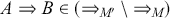

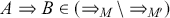
(defeat) expresses that there is an attack from  to
to  which is undefendable, while (defense) expresses that every attack from
  to
to  can be defended. In terms of the preceding described argumentative reading, the two conditions describe winning conditions for the proponent of
  when arguing with an opponent favoring
  .
.
Definition 13.2. In case there is a unique  -minimal model
  among all ranked models of a given set of defaults
  ,
,  is called the rational closure of
  .Footnote 54
Example 50 (Exaple 49 cont.). We consider models  and
and  in Fig. 29. We have
  . (defeat) holds since

Also (defense) holds, for example, where  , although
  , there is

We now discuss an alternative characterization of the rational closure in terms of ranking sentences according to their normality (relative to  ). This will also help defining a significant class of sets of defaults for which the rational closure exists, so-called admissible sets (see Proposition 13.1). For this we inductively associate sentences with ordinals via a function
  . We say that a sentence
  is exceptional for
  in case
  , so in case
  expresses that normally
  is false. Similarly,
  is exceptional for
  if
if  is exceptional for
  . We collect the exceptional defaults in
  in the set
  . Where
  , we let
  for all successor ordinals
  and
and  for all limit ordinals
  . Now, some sentence
  has a rank for
  in case there is a least ordinal
  for which
  is not exceptional for
  , in which case the rank of
  is
is  . Otherwise,
  has no rank.Footnote 55
Example 51 (Example 50 cont.). For all  ,
,  and
and  are not exceptional for
  and so have rank 0. Exceptional for
  are, for instance,
  and
and  . These formulas have rank 1.
We call a set  admissible if for every sentence
  that has no rank,
  . Examples for admissible sets are sets
  based on a finite language (a language with only finitely many atoms), or for which the preferential closure has no infinite sequences of more and more normal sentences.
Proposition 13.1 (Lehmann and Magidor (1990). Where  is admissible, the rational closure of
  exists and it consists of all
  for which
  has no rank, or for which
  .
.
Example 52 (Example 51 cont.). In view of Proposition 13.1, for instance,  is in the rational closure of
  since
since  has rank 0 while
  has rank 1.
However,  is not in the rational closure of
  since
since

have the same rank, namely 1. This shows that rational closure “suffers” from the drowning problem (see Section 1.2): since nonvegans are exceptional with respect to  , they turn out exceptional also with respect to
  .Footnote 56
14 Quantitative Methods
So far, we have interpreted  as
as  holds in the most normal situations in which
  holds (recall (⋆)). According to a similar idea:
- ()
- holds if, given , is more normal/plausible/etc. than .


The notion of normality was rendered precise in terms of a preference order on the logically possible situations. Instead of this qualitative approach, one may follow the idea behind  but proceed quantitatively and interpret
  in terms of probabilities: given
  ,
,  is more probable than
  . In what follows we introduce the central approach to probabilistic semantics by Adams (Reference Adams1975), which corresponds to system
  .Footnote 57
14.1 Adams’ Approach: -Semantics

We again consider a set of situations  interpreted via an assignment
  .Footnote 58
We now equip  with a probability function
  which maps sets of situations into
  such that (1)
  and (2) for any pairwise disjoint
  ,
,  . We call each
  a probabilistic model. For every formula
  , a probabilistic model provides information of how probable it is to be in a situation consistent with
  . Where
  (we skip the subscript when the context disambiguates), we will write
  instead of
  for the formal expression of this information. The conditional probability
  is, as usual, defined by
  in case
  (otherwise, it is undefined). It expresses the probability of being in a situation in which
  holds, given that
  holds.
Example 53. Let  , where
  stands for ‘being a bird’,
  for ‘flying’ and
  for ‘having wings’. The probabilistic models
  and
and  are given by Table 11.
We have, for instance,  ,
,  and therefore
  , while
  ,
,  and
and  .
.

Table 11Long description
The table consists of six columns: situations; s Double Turnstile b; s Double Turnstile f; s Double Turnstile w; p subscript 1; and p subscript 2. It read as follows: Row 1: s subscript 1; checkmark; Blank; Blank; dot 2; dot 1. Row 2: s subscript 2; checkmark; Blank; checkmark; dot 2; dot 1. Row 3: s subscript 3; checkmark; checkmark; Blank; dot 2; dot 2. Row 4: s subscript 4; checkmark; checkmark; checkmark; dot 4; dot 2. Row 5: s subscript 1 prime; Blank; Blank; Blank; 0; dot 1. Row 6: s subscript 2 prime; Blank; Blank; checkmark; 0; dot 1. Row 7: s subscript 3 prime; Blank; checkmark; Blank; 0; dot 1. Row 8: s subscript 4 prime; Blank; checkmark; checkmark; 0; dot 1.
We now define when a default  holds in a given probabilistic model
  (in signs,
  ). A consequence relation can then be defined as follows. Where
  is a set of defaults:
  iff for all probabilistic models
  of
of  ,
,  .Footnote 59 Before moving to Adams’ approach, we state three naive ideas. Let
  .
.
Naive 1
, iff or if .Footnote 60Naive 2
, iff or if .Naive 3
, iff for some threshold value (such as ), or if .Footnote 61


We note that approaches Naive 1 and Naive 2 are equivalent since, in case  :
:  , iff
, iff  , iff
, iff  . The weakness of the preceding naive approaches can be illustrated by applying them to our example.
Example 54 (Example 53 cont.). Let  . In model
  we have
  which is why
  . Similarly,
  , which is why
  . However, since
  , we also have
  , even
  .
.
This means that AND is violated for the induced consequence relation. This model allows for a situation where  , albeit
  is an inconsistent set. Similarly, other central properties of nonmonotonic entailment, such as CT, fail in our naive approaches.
In view of these weaknesses, Adams introduced another approach. In his semantics the degree of assertability of  is modelled by the conditional probability
  . In a nutshell, the central idea is that some
  is entailed by a set of defaults
  in case its assertability approximates 1 when the elements of
  are being interpreted as increasingly assertable. In formal terms, let
  be a proper probability function for
  in case
  for all
  . We define:
Definition 14.1 (ϵ-entailment, Adams, 1975; Pearl, 1989). Let  be a set of defaults. We define:
  , iff, for any
  , there is a
  such that for all proper probability functions
  for
for  : if, for all
  ,
,  , then
  .
.
Does this approach lead to a more well-behaved entailment relation and what are characteristic properties of  -entailment? Let us have another look at our example.
Example 55 (Example 54 cont.). Where  , we have, for instance,
  . In order to show this, let
  be arbitrary and consider a probability function
  . We need to find a
  such that if
  , then
  . Let
. Let  and suppose that
  . Then,

What we have just shown in the context of our example is not coincidental. Indeed, the proof of AND for  -entailment follows exactly the structure of the proof in Example 55. What is more,
  -entailment can be shown to coincide with system
  for finite knowledge bases (Geffner, Reference Geffner1992; Lehmann & Magidor, Reference Lehmann and Magidor1990): a remarkable correspondence between two rather different perspectives on the meaning of
  .
.
14.2 Other Quantitative Approaches
We close this section with some pointers to related approaches. While in Adams’ approach we find a probabilistic characterization of  -entailment, the reader may wonder whether also
  -entailment can be represented by a quantitative approach. Indeed, utilizing a nonstandard probabilistic approach including infinitesimal values, Lehmann and Magidor (Reference Lehmann and Magidor1992) present a variant of Adams’ system that characterizes rational entailment.
Instead of probability measures other quantitative measures have been utilized in the literature to give meaning to defaults. We let  again be a finite set of situations and
  an assignment function.
A possibility measure (Dubois & Prade, Reference Dubois, Prade, Shafer and Pearl1990)
determines the possibility of a set of situations, from impossible (0) to maximally possible (1).Footnote 62 It is required that , , and for any , . A possibilistic model is of the form .An ordinal ranking function (Goldszmidt & Pearl, Reference Goldszmidt and Pearl1992; Spohn, Reference Spohn, Harper and Skyrms1988)
associates each set of situations with a level of surprise, from unsurprising (0) to shocking (). It is required that , , and, for any , . An ordinal ranking model is of the form .


It is easy to see that letting  iff
iff  in the context of a possibilistic model
  [resp. iff
  in the context of an ordinal ranking model
  ] gives rise to a ranked model
  .
.
In each of these approaches the meaning of defaults in a given model is defined analogous to the underlying idea of ( ):
):
Where
is a possibilistic model, we let iff or Where
is an ordinal ranking model, we let iff or .


We say that a possibilistic model [resp. an ordinal ranking model]  is a model of a set of defaults
  in case
  for all
  .
.
For instance, a possibilistic model verifies  just in case
  is impossible, or if
  is strictly more possible than
  . Since ranking functions model the level of surprise an agent would face when learning that some
  is true, according to a ranking function
  is valid in case
  would cause maximal surprise or if learning about
  would cause strictly less surprise than learning about
  .
.
Example 56 (Ex. 53 cont.). We consider the set of states  in Example 53. Fig. 30 shows a cardinal ranking function
  and a possibility function
  . Recall that for
  ,
,

which is why the figure fully characterizes  and
and  by illustrating what values are assigned to single states. Where
  and
and  , we have:
- since
- since
- since , and
- since .


Figure 30 Example 56. (Left) The cardinal ranking  . (Right) The possibility function
  .
.
Entailment relations are induced in the usual way. Given a set of defaults  , we let
- iff for all possibilistic models of , ,
- iff for all ordinal ranking models of , .


It is a most astonishing result in NML that all these different perspectives lead exactly to a characterization of  -entailment, a result that strongly underlines the central character of its underlying reasoning principles.
Theorem 14.1 (Dubois and Prade, 1991; Geffner, 1992; Lehmann and Magidor, 1992). Let  be a finite set of defaults. We have:
  iff
iff  iff
iff  iff
iff  iff
iff  .
.
15 A Preferential Semantics for Some NMLs
In this section we present a preferential semantics for logics based on temperate accumulation and knowledge bases of the type  ,Footnote 63 such as Rescher and Manor’s logics based on maxicon sets and Makinson’s default assumptions (see Section 11.3.1).
In fact, this is exactly the semantics we introduced in Section 5.3, so our main aim in this section is to show its adequacy for temperate accumulation. We refer to Example 21, 22 in Section 5.3 for an illustration of this idea.
Let us briefly recall the general setup. We work in the context of a Tarski logic  (such as classical logic) which has an adequate model-theoretic semantic representation: for any set of
  -sentences
  it holds:
  iff for all
  -models
  of
of  (i.e., for all
  ,
,  ) it is the case that
  . In particular, we assume that the consistency of a set of sentences
  can be expressed by
  .
.
In order to determine whether  defeasibly follows from
  , we compare the
  -models of the strict assumptions
  in terms of how normal they interpret the defeasible assumptions in
  . For this, we consider the normal part of a given model
  , which is simply the subset of defeasible assumptions it validates:
  . Now we define an order on the
  -models of
  by:
by:

We select the most normal models of  and define a consequence relation
  by:
by:

In the following we show how  and
and  can be characterized by a semantics based on
  .Footnote 64 For this we make use of the characterization of temperate accumulation in terms of maxicon sets (see Lemma 10.1 and Theorem 10.1).
Theorem 15.1. Let  be a knowledge base. Then,
  iff
iff  .
.
The theorem follows in view of the following lemmas.
Lemma 15.1. For every  ,
,  .
.
Proof. Suppose that  and let
  . Thus,
  is consistent. Consider some
  for which
  is consistent and
  . Thus, there is a
  . Since
  ,
,  and by the
  -minimality of
  ,
,  . Thus,
  . □
. □
Lemma 15.2. For every  there is an
  for which
  .
.
Proof. Suppose  . By the consistency of
  , there is an
  . Consider a
  for which
  . Then
  is consistent. Since
  and the maximality of
  ,
,  . So,
. So,  and thus,
  . □
. □
Proof of Theorem 15.1  , iff [by Proposition 11.3], for all
  ,
,  , iff [by Lemmas 15.1 and 15.2], for all
  ,
,  , iff,
  . □
. □
We now move on to characterize  semantically. We can capture this consequence relation by defining a threshold function
  on the degree of normality a selected model is allowed to have.

So the core of  consists of those models whose normal part contains at least all those sentences that are part of the normal parts of every
  -minimal model. Clearly, each
  -minimal model belongs to the core, but possibly also other models. Let, moreover,

Given that  , the consequence relation
  will typically give rise to a more cautious reasoning style than
  .
.
Example 57 (Example 21 cont.). For our  with
with

and  we have three minimal models:
  with
with  ,
,  with
with  , and
, and  with
with  (see Fig. 12). So,
  and therefore
  , and
, and  iff
iff  . This highlights the fact that
  leads to a more cautious reasoning style than
  .
.
We now consider  , where
  . In Fig. 31 we highlight the models in
  . In this case
  . This is reflected, for instance, in the consequences
  while
while  , and
, and  while
while  .
.

Figure 31 The order  on the models of
  in Example 57. Highlighted are the models in
  . The atoms
  , and
, and  are true in every model of
  .
.
With Lemmas 15.1 and 15.2 we immediately get:
Corollary 15.1. Let  be a knowledge base and
  . Then,
  iff
iff  .
.
Theorem 15.2. Let  be a knowledge base. Then,
  iff
iff  .
.
Proof. Suppose  . Thus, by Proposition 11.3,
  . Let
. Let  . By Corollary 15.1,
  and so
  . Thus,
  . So,
. So,  .
.
Suppose  . Thus, by Proposition 11.3,
  . So, there is a
  such that
  . So,
. So,  . By Corollary 15.1,
  . So,
. So,  . □
. □
Combining our previous results with the result in Proposition 11.3, we get:
Corollary 15.2. Let  be a knowledge base. Then,
1.
iff iff .2.
iff iff .


16 Logic Programming
Logic programming is a declarative approach to problem solving. The idea is that a user describes a given reasoning problem by means of a so-called logic program in a simple syntax, without the need of encoding an algorithm to solve the problem. Automated proof procedures or semantic methods are then used to provide answers to queries. With the addition of negation-as-failure(-to-prove) (Section 16.1) or default negation, logic programming became a key paradigm in NML. It gave rise to a rich variety of applications, from legal reasoning (Sergot et al., Reference Sergot, Sadri, Kowalski, Kriwaczek, Hammond and Cory1986), to planning (including applications for the Space Shuttle program in Nogueira et al. (Reference Nogueira, Balduccini, Gelfond, Watson and Barry2001)), to cognitive science (Stenning & Van Lambalgen, Reference Stenning and Van Lambalgen2008), and others. In this section we will introduce one of the central semantical approaches based on stable models (Section 16.2), which under the addition of classical negation became known as answer set programming (in short: ASP, Section 16.3). In Section 16.4 we note that ASP and default logic coincide under a translation and that ASP can be considered a form of formal argumentation.
16.1 Normal Logic Programs and Default Negation
A logic program in its simplest form is a collection of strict inference rules of the form
 (16.1.1)
where  are atomic formulas (incl.
  or
or  ).Footnote 65 These rules are called the clauses of the program. Factual information is represented by rules with empty bodies, such as
  . We reason with such programs as one would expect:
  follows from a program
  just in case there is an argument based on
  with the conclusion
  (recall Definition 5.1).
Similar to default logic, logic programming also accommodates defeasible assumptions in the body of rules such as:
On Sunday mornings Jane goes jogging, except it is stormy.
In logic programming the “except …” part is expressed with a dedicated negation  whose exact interpretation we discuss as follows:
 (16.1.2)
More generally, we are now dealing with rules of the form
 (16.1.3)
where  are atomic formulas. Sets of rules
  of the form (16.1.3) are called normal logic programs. The technical term for
  is “negation-as-failure(-to-prove)” or simply “default negation.” The basic idea is that
  is considered true in the context of
  unless there is an argument for
  (based on
  ). So,
  is entailed by the program only consisting of the rule (16.1.2), but if we add
  it should not be entailed.
How to define a nonmonotonic consequence relation for negation-as-failure? Prima facie, the following simple (but ultimately flawed) idea seems to be in its spirit. We consider arguments that can be built with the rules in the given program  and that are based on defeasible assumptions of the type
  . Let for this
  be all formulas of the type
  , where
  occurs in some rule in
  and let
  be the knowledge base consisting of the defeasible assumptions
  and the strict rules in
  . So
. So  is of the form
  , or in shorter notation
  . We then let an atom
  be entailed by
  just in case the following two criteria are fulfilled:
1. there is an argument
for in (recall Definition 5.1), and2. there is no argument for
in for any occurring in .


This would allow us to conclude  from
from

The reason is that, where  , there is an argument
  in
in  for
for  , namely
  , and there is no argument for
  in
in  . At the same time, this approach blocks the conclusion
  from
from  since now there is an argument
  for
for  in
in  , where
  .
.
However, we run quickly into problems with our naive approach once the logic programs are slightly more involved.
Example 58. Consider, for instance, the following logic program:

In this case, although it seems reasonable to infer  , our naive approach doesn’t permit it. To see this, we observe that the argument
  for
for  relies on the assumption
  . Although
  can be concluded in view of a (counter-)argument
  based on the assumption
  , the latter is problematic since
  follows strictly in
  by the argument
  . This kind of reinstatement, in which an attacked argument is successfully defended by a nonattacked argument, cannot be handled by our naive approach.Footnote 66
Several ways that deal with such and similar problems have been proposed in various semantics for logic programming (see e.g., Eiter et al. (Reference Eiter, Ianni and Krennwallner2009)). In the following we will focus paradigmatically on one of the central approaches based on so-called stable models (Gelfond & Lifschitz, Reference Gelfond and Lifschitz1988).
16.2 Stable Models
A way to tackle the problem of reasoning with logic programs that contain default negation is by considering interpretations of programs. Let us start with the simple case of a  -free logic program
  consisting of rules of the form (16.1.1). A model
  of
of  is a function that associates each atom
  occurring in a rule in
  with true (written
  ) or false (written
  ). As usual, we let
  and
and  . Where
  , we write
  (“
(“ validates
  ”) in case
  , …,
, …,  implies
  . A compact representation is by letting
  be the set of those atoms in
  that it interprets as true (and so
  iff
iff  ).Footnote 67
Example 59. Let  and consider
  ,
,  ,
,  , and
, and  . Then,
  ,
,  , and
, and  are not models of
  :
:  and
and  violate the first rule (since
  and
and  ) and
) and  violates the second rule (since
  although
  ). The only model of
  is
is  .
.
It is easy to see that a  -free program
  has a minimal model, that is, a model
  of
of  such that for all other models
  of
of  ,
,  . In fact, as the reader can easily verify, the minimal program will consist exactly of the conclusions of arguments based on the rules in
  .
.
Fact 16.1. Let  be a
be a  -free program. Then,
  is the minimal model of
  .
.
As we have seen in the previous section, things get more interesting when we also consider default negation  . For this we adjust the notion of validity in a model.
Definition 16.1. Let  be a set of atoms. We let
- , iff, or and
- , iff, .


Where  is a rule of type (16.1.3),
- , iff, , …, , , …, implies .


We write  for the set
  and
and  for the set of atoms occurring in
  .
.
Let  be a normal logic program and
  . We say that
  is a model of
  in case
  for all
  . We write
  for the set of all models of
  .
.
By having another look at  we note that not all models of a given program are equally representative of a rational reasoner.
Example 60 (Example 58 cont.). We consider the following candidates for models of  :
:

We have  for
for  and
and  .
.  is not a model of
  since
since  .
.  and
and  are models of
  .
.
However, we also notice problems with  . In particular we have
  , although the only argument for
  based on
  is
is  while
while  . So,
. So,  is “unfounded” in
  : it is valid but not supported by an argument in
  . A desideratum for us will thus be that models
  of a program
  are founded in these programs in the sense that every atom contained in
  can be inferred by means of
  and the defeasible assumptions
  in
in  . Let us make this precise.
Definition 16.2. Let  be a normal logic program and
  be a model. We let
  be the knowledge base consisting of the defeasible assumptions in
  and the rules in
  . A model
  of
of  is founded (in
  ) if for each
  there is an argument
  with conclusion
  (so,
(so,  ).
).
In order to filter out unfounded models, Gelfond and Lifschitz (Reference Gelfond and Lifschitz1988) have proposed the concept of a reduction program.
Definition 16.3. Given a model  of
of  , we let the reduction of
  by
by  , written
  , be the result of (i) replacing each occurrence of a
  -negated formula
  in
in  by
by  in case
  and by
  else, and of (ii) adding the rule
  .
.
Definition 16.4. Let  be a normal logic program.
  is a stable model of
  in case it is identical to the minimal model of
  . We write
  for the set of stable models of
  .
.
It is reassuring to note that (a)  is a
is a  -free program and therefore has a minimal model (see Fact 16.1), and (b) if
  is a model of
  , then it is also a model of
  .
.
Lemma 16.1. Let  and
and  . Then,
  .
.
Proof. Let  such that
  and
and  for each
  . Thus,
  . Since
  ,
,  . □
. □
Example 61 (Example 60 cont.). Let us put this idea to a test with  and the two models
  and
and  .
.

Table 010Long description
The table consists of three columns: pi constant subscript 2; pi constant subscript 2 superscript M subscript 1; and pi constant subscript 2 superscript M subscript 2. It read as follows: Row 1: not q right arrow r; Top right arrow r; Bottom right arrow r. Row 2: not s right arrow q; Bottom right arrow q; and Bottom right arrow q. Row 3: right arrow s; right arrow s; and right arrow s. Row 4: Blank; right arrow Top; and right arrow Top.
The minimal model of  is
is  , the minimal model of
  is
is  . So, as expected, while
  is a stable model of
  ,
,  is not.
Stable models do not exist for every program. Indeed, for some logic programs the only existing models are unfounded ones.
Example 62. A case in point is  . Note that
  is not a model of
  since
since  and so
  would have to be true in
  to be a model of
  . So we are left with
  . But this model is not founded.Footnote 68
Programs containing conflicts may give rise to several stable models.
Example 63. As a simple example, consider  .
.  is not a model of
  , since both rules are applicable in
  , but
, but  . On the other hand,
  is not minimal (and hence unfounded), since neither rule is applicable in
  . We are left with
  and
and  . As the reader can easily verify, these two models are stable.
16.3 Extended Logic Programs and Answer Sets
So far we have limited our attention to a rather weak language, only consisting of atoms and their default negations. We now will add another negation  to the mix which will behave more similar to classical negation. This puts us in the realm of extended logic programs, which are sets of rules of the form
 (16.3.1)
where  are
are  -literals, that is, atoms or
  -negated atoms.
  denotes the set of all
  -literals occurring in an extended program
  .
.
It is our task now to enhance the notion of a model to extended programs. A simple way is by means of a translation  of a given extended program
  to a normal program
  (Gelfond & Lifschitz, Reference Gelfond and Lifschitz1991) in which each occurrence of some
  is replaced by a new atom
  (not occurring in
  ). We then consider only those models
  of
of  for which
- or for all atoms or
- contains all and for all atoms in .Footnote 69


We then translate  back by considering
  , replacing atoms of the form
  by
by  . If
. If  is a stable model of
  then we define
  to be a stable model of
  . The latter are also known as answer sets of
  .
.
Of course, we can also define a nonmonotonic consequence relation based on answer sets: where  is a
is a  -literal, or a
  -negated
  -literal and
  is an extended logic program we let:

Example 64. We consider the extended logic program  consisting of:

In the translated program  , rules 1 and 2 are replaced by:

We have two stable models of  , as the reader can easily verify by inspecting Table 12.

So, the answer sets of  are
are  and
and

We note that  , but
, but  and
and  . This shows that negation-as-failure as interpreted in answer set programming does not realize a closed-world assumption in the strong sense that every atom
  that is not derivable is interpreted as strongly negated,
  .Footnote 70
If we add the additional rule  to
to  , resulting in
  , we end up with one answer set, namely

In terms of nonmonotonic consequence we have
- , while , and
- , while and .


Table 12Long description
The table consists of five columns: M subscript 1, M subscript 2, M subscript 3, M subscript 4, and M subscript 5. It read as follows: Row 1: working: checkmark, checkmark, checkmark, checkmark, checkmark. Row 2: Sunday Morning: checkmark, checkmark, checkmark, checkmark, checkmark. Row 3: jogging: checkmark, Blank, Blank, checkmark, checkmark. Row 4: jogging prime: Blank, checkmark, checkmark, Blank, checkmark. Row 5: stormy: Blank, Blank, checkmark, checkmark, checkmark. Row 6: r subscript 1 prime: checkmark, checkmark, checkmark, checkmark, checkmark. Row 7: r subscript 2 prime: checkmark, checkmark, checkmark, checkmark, checkmark.
Example 65. There are extended programs with only inconsistent (stable) models, for example, 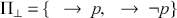 . The only model of
  is
is  . So the only model of
  is
is  .
.
16.4 Answer Sets, Defaults, and Argumentation
Answer sets are closely related to the extensions of Reiter’s default logic (Section 12.2).Footnote 71 We can translate a clause of the form (16.3.1) to a (possibly) nonnormal default by

where for an atom  ,
,  and
and  . Let the resulting translation of an extended program
  be
be

Example 66. We have 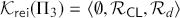 , where
  consists of the following general default rules:

Theorem 16.1 (Gelfond and Lifschitz, 1991). Let  be an extended program and
  . Then,
1. if
, then , and2. for every
there is exactly one for which .


Given this result the metatheoretic results for Reiter’s greedy approach immediately apply (see Section 12.1), such as cautious transitivity for  .Footnote 72
In the following we show that answer sets can also be expressed in logical argumentation.Footnote 73 We will improve our previous naive attempt (see Section 16.1 and recall the problematic Example 58) by allowing for reinstatement.
Definition 16.5. Let  be an extended logic program. We let
  , where
  and for
  , we let
  attack
  (in signs
  ) if there is a sub-argument
  of
of  such that
  .
.
Example 67 (Example 64 cont.). We consider  and list arguments in
  that give rise to the argumentation framework in Fig. 32 (left).

Table 011Long description
The list describes: 1. a subscript zero equals right arrow working; 2. a subscript one equals right arrow Sunday Morning; 3. b subscript one equals similarity jogging; 4. b subscript two equals similarity not jogging; 5. b subscript three equals similarity stormy; 6. c subscript one equals (a subscript one, b subscript two, b subscript three right arrow jogging); 7. c subscript two equals (a subscript zero, b subscript one right arrow not jogging).
We obtain two stable extensions of  :
:

The set of conclusions (in  ) of arguments in the two stable models correspond to the two answer sets of
  , namely:


Figure 32 Argumentation framework for Examples 67 (left) and 68 (right). We omit nonattacked arguments.
Example 68 (Example 58 cont.). We consider the problematic example for our naive argumentation-based account,  . We have the following arguments in
  , giving rise to the argumentation framework in Fig. 32 (right).
The unique stable extension of  is
is  (highlighted). The set of atoms in
  is identical to the only stable model of
  , namely
  .
.

Table 012Long description
The table consists of three columns. It read as follows: Row 1: a subscript 1 not s; b subscript 1 equals right arrow s; b subscript 2 equals a subscript 1 right arrow q. Row 2: a subscript 2 equals not q; blank; b subscript 3 equals a subscript 2 right arrow r.
The correspondence is not coincidental. For a given extended logic program  let
let  be the set of consistent answer sets of
  , that is, those stable models of
  that do not contain contradictory literals.Footnote 74
Theorem⋆ 16.2. Let  be an extended logic program.
1. If
, then .2. If
and , then .


Selected Further Readings
Friedman and Halpern (Reference Friedman and Halpern1996) provided a unifying approach to default reasoning based on plausibility orders covering many of the previously mentioned NMLs, such as the preferential semantics of Kraus et al. (Reference Kraus, Lehman and Magidor1990), the possibilistic approach by Benferhat et al. (Reference Benferhat, Dubois, Prade, Nebel, Rich and Swartout1992), ordinal rankings by Spohn (Reference Spohn, Harper and Skyrms1988), and  -semantics (Adams, Reference Adams1975; Pearl, Reference Pearl1989). Another generalization is provided in Arieli and Avron (Reference Arieli and Avron200), who go beyond a classical base logic. Preferential conditionals have been embedded in the scope of a full logical language (so that they are allowed to occur in the scope of logical connectives such as
  ) in conditional logics (Asher & Morreau, Reference Asher, Morreau and van Eijck1991; Boutilier, Reference Boutilier1994a; Friedman & Halpern, Reference Friedman and Halpern1996). First-order versions of preferential consequence relations and conditional logics have been investigated, for example, in Delgrande (Reference Delgrande1998; Friedman et al. (Reference Friedman, Halpern and Koller2000) and Lehmann and Magidor (Reference Lehmann and Magidor1990). Proof theories for conditional logics in the style of Kraus et al. (Reference Kraus, Lehman and Magidor1990) can be found in Giordano et al. (Reference Giordano, Gliozzi, Olivetti and Pozzato2009), and for rational closure in Straßer (Reference Straßer, Carnielli and D’Ottaviano2009b) in terms of adaptive logics. Deep connections between preferential approaches and belief revision have been observed in many places, for example, Boutilier (Reference Boutilier1994b), Gärdenfors (Reference Gärdenfors1990), Rott et al. (Reference Rott2021).
Logics based on preferential semantics and logic programming have been characterized in terms of artificial neural nets; see for example Besold et al. (Reference Besold, d’Avila Garcez, Stenning, van der Torre and van Lambalgen2017), Hölldobler and Kalinke (Reference Hölldobler and Kalinke1994), and Leitgeb (Reference Leitgeb2018).
An overview and introduction to logic programming with an emphasis on answer sets is, in book form, Lifschitz (Reference Lifschitz2019), and more compactly, Eiter et al. (Reference Eiter, Ianni and Krennwallner2009). As the reader will expect, many variants of logic programming exist, including disjunctions (Minker, Reference Minker1994), preferences (Schaub & Wang, Reference Schaub and Wang2001), probabilities (Ng & Subrahmanian, Reference Ng and Subrahmanian1992) with connections to deep learning (Manhaeve et al., Reference Manhaeve, Dumanéiæ, Kimmig, Demeester and De Raedt2021), and so on. Logic programming has been successfully applied in the psychology of reasoning (Saldanha, Reference Saldanha2018; Stenning & Van Lambalgen, Reference Stenning and Van Lambalgen2008).
Acknowledgments
I want to thank Kees van Berkel, Matthis Hesse, Jessica Krumhus, and Dunja Šešelja for their highly valuable feedback on previous drafts. I am also much obliged to Joke Meheus and Diderik Batens for introducing me to the wonderful world of NMLs. Finally, not to forget Brad and Fred: thanks to my editors, Brad Armour-Garb and Fred Kroon, for their support, trust, and good mood throughout the whole process.
SUNY Albany
Bradley Armour-Garb is chair and Professor of Philosophy at SUNY Albany. His books include The Law of Non-Contradiction (co-edited with Graham Priest and J. C. Beall, 2004), Deflationary Truth and Deflationism and Paradox (both co-edited with J. C. Beall, 2005), Pretense and Pathology (with James Woodbridge, Cambridge University Press, 2015), Reflections on the Liar (2017), and Fictionalism in Philosophy (co-edited with Fred Kroon, 2020).
The University of Auckland
Frederick Kroon is Emeritus Professor of Philosophy at the University of Auckland. He has authored numerous papers in formal and philosophical logic, ethics, philosophy of language, and metaphysics, and is the author of A Critical Introduction to Fictionalism (with Stuart Brock and Jonathan McKeown-Green, 2018).
About the Series
This Cambridge Elements series provides an extensive overview of the many and varied connections between philosophy and logic. Distinguished authors provide an up-to-date summary of the results of current research in their fields and give their own take on what they believe are the most significant debates influencing research, drawing original conclusions.