


1. Introduction
Following the ever-increasing development and complexity of the financial market, credit rating migration risk is playing a more and more important role. The 2008 financial tsunami and 2010 European debit crisis exemplify the importance of proper credit risk management. It gradually becomes an urgent task both for industries and academics to measure and manage the risk [Reference Chen, Dai and Wan5, Reference Dai, Huang and Keppo6]. In theory, there are two main mathematical frameworks for this risk: structure model and intensity one. They are different, one modelled by endogenic causes and the other by exogenous factors.
Structural models involve the reason of the rating objects themselves and usually indicate the rating migration boundaries; therefore, they have some advantages. The works using this kind of model for credit rating migration can be found in [Reference Chen, Hu, Liang and Yin4, Reference Fu, Chen and Liang7, Reference Hu, Liang and Wu10, Reference Liang, Wu and Hu12–Reference Yin, Liang and Wu17] and the reference therein, where a credit migration boundary is used for both upgrading and downgrading. The stochastic feature of the model will then create a phenomena of infinite many upgrading and downgrading since any Brownian motion path oscillates around any level it reached infinitely many times. Thus, a model equipped with a buffer zone, called dead band or hysteresis, is necessarily needed.
In [Reference Chen and Liang3], we establish a model for credit rating migration with different migration upgrading and downgrading thresholds. In the model, credit rating migrations are assumed to depend on the ratio of debt and asset value of the underlying company where debt is assumed to be a zero coupon corporate bond and asset value follows a geometric Brownian motion with volatility depending on credit rating. There is a buffer zone in credit rating migration, so upgrade and downgrade thresholds are different. Mathematically, this model is a system of partial differential equations (PDEs) with two free boundaries that correspond to the hitting boundaries in state space to upgrade and downgrade credit rating, respectively. Under the condition of zero dividend, the existence, uniqueness, regularity and asymptotic behaviour of the solution and free boundaries are obtained. In addition, some nonzero dividend cases are discussed on the behaviours of the solution. However, the existence and uniqueness of the solution in the nonzero dividend case are still open, since the method for the zero dividend case seems to be no more suitable for the nonzero dividend case. In this paper, we are going to fill this gap.
From the discussion of the asymptotic behaviour of the nonzero dividend case in [Reference Chen and Liang3], we see that the migration free boundaries will go to negative infinite time. This adds an interesting phenomena to the model. There exist two times, $T^L$
and
$T^L$
and $T^H$
with
$T^H$
with $0\lt T^H\lt T^L$
. When time to expiry is larger than
$0\lt T^H\lt T^L$
. When time to expiry is larger than $T^L$
, the credit rating is always high. When time to expiry is between
$T^L$
, the credit rating is always high. When time to expiry is between $T^H$
and
$T^H$
and $T^L$
, the credit rating can change at most once and it is from low to high. Only when the time is shorter than
$T^L$
, the credit rating can change at most once and it is from low to high. Only when the time is shorter than $T^H$
, there are credit rating changes that go both directions.
$T^H$
, there are credit rating changes that go both directions.
However, the method in [Reference Chen and Liang3] cannot be directly applied to the nonzero dividend case, as one PDE with nonzero dividend in the buffer zone is no longer suitable to the maximum principle. That means, the upgrade/downgrade condition might be violated in the buffer zone. Thus, the old model for nonzero dividend needs to be modified. To avoid the ratios run out the threshold inside the buffer zone, obstacle problems are applied to the model instead of pure PDEs.
The paper is organised as follows. In Section 1, a model with nonzero dividend is presented, with the model in [Reference Chen and Liang3] being a special case. In Section 3, a priori properties of the solution of our model are discussed; in particular, it is shown that, when dividends are positive, two free boundaries go to $-\infty$
in finite time. In Section 4, some preparations for theoretical proofs are made. In Section 5, we construct two monotonic sequences of super and subsolutions and prove that both sequences approach the unique solution of the problem. Since the free boundaries go to
$-\infty$
in finite time. In Section 4, some preparations for theoretical proofs are made. In Section 5, we construct two monotonic sequences of super and subsolutions and prove that both sequences approach the unique solution of the problem. Since the free boundaries go to $-\infty$
, part of the solutions are limited to finite time to have a financial meaning. Main theorem is stated in Section 6, where uniqueness is also proved. Section 7 gives final conclusion.
$-\infty$
, part of the solutions are limited to finite time to have a financial meaning. Main theorem is stated in Section 6, where uniqueness is also proved. Section 7 gives final conclusion.
2. Model
A credit rating migration model is established in [Reference Chen and Liang3], where only Black–Scholes equations are used. When underlying asset pays zero dividend, the model was shown to be well-posed. When positive dividends are added into the model, only short-time existence can be proved and global solutions do not exist in certain cases. Hence, the model in [Reference Chen and Liang3] needs to be modified. In this paper, we revise the model by replacing the Black–Scholes equations by variational inequalities. We will show later that the revised model is well-posed.
2.1. Basic assumptions
We assume that the underlying firm issues a corporate bond, which is a contingent claim of its (observable) asset value and its credit rating. We consider the simple case where only two ratings are used: “H” and “L”.
Assumption 1 (Firm’s asset under different credit ratings). Let $(\Omega,\{\mathcal{F}_t\}_{t\geqslant 0},P)$
be a complete probability space with filtration. Denoting by
$(\Omega,\{\mathcal{F}_t\}_{t\geqslant 0},P)$
be a complete probability space with filtration. Denoting by $S_t$
the firm’s asset value in the risk neutral world,
Footnote
1
we assume that
$S_t$
the firm’s asset value in the risk neutral world,
Footnote
1
we assume that $\{S_t\}$
obeys the stochastic differential equation (SDE)
$\{S_t\}$
obeys the stochastic differential equation (SDE)
 \begin{equation} \frac{dS_t}{S_t}=\left \{\begin{array}{l@{\quad}l}(r-\delta ^H) dt+\sigma ^H dW_t\quad &\mbox{ in the high rating region,}\\[5pt] (r-\delta ^L) dt+\sigma ^L dW_t\quad &\mbox{ in the low rating region,}\end{array}\right . \end{equation}
where $r$
is the risk free interest rate, and
$r$
is the risk free interest rate, and $({\sigma }^H,{\sigma }^L)$
and
$({\sigma }^H,{\sigma }^L)$
and $(\delta ^H,\delta ^L)$
are constants that represent volatilities and dividend rates of the firm under the high and low credit grades, respectively. Also
$(\delta ^H,\delta ^L)$
are constants that represent volatilities and dividend rates of the firm under the high and low credit grades, respectively. Also $\{W_t\}_{t\geqslant 0}$
is the standard Brownian motion, which generates the filtration
$\{W_t\}_{t\geqslant 0}$
is the standard Brownian motion, which generates the filtration $\{{\mathcal{F}}_t\}$
.
$\{{\mathcal{F}}_t\}$
.

Figure 1. An illustration of the rating migration. Left: starting from a low rating, the rating will upgrade at $\tau _1$
, downgrade at
$\tau _1$
, downgrade at $\tau _2$
, upgrade at
$\tau _2$
, upgrade at $\tau _3$
and downgrade at
$\tau _3$
and downgrade at $\tau _4$
; Right: with the same sample path as the left, but starting from a high rating, the rating will downgrade at
$\tau _4$
; Right: with the same sample path as the left, but starting from a high rating, the rating will downgrade at $\tau _0$
, the rest is the same as the left figure. Starting from different rating, the bond values are different only up to time
$\tau _0$
, the rest is the same as the left figure. Starting from different rating, the bond values are different only up to time $\tau _0$
. After
$\tau _0$
. After $\tau _0,$
initial difference of company’s rating disappears.
$\tau _0,$
initial difference of company’s rating disappears.
In this paper, we assume that
 \begin{equation} 0\lt \sigma ^{H}\lt \sigma ^{L}, \quad 0\leqslant \delta ^L\leqslant \delta ^H. \end{equation}
This means that the volatility in the high rating region should be lower than the one in low rating region, and in high rating, the firm would like to pay more dividend.
When $\delta ^L=\delta ^H=0,$
as one can see from our analysis, no variational inequalities are needed, so the model reduces to the one in [Reference Chen and Liang3]. Hence, in this paper, we consider only
$\delta ^L=\delta ^H=0,$
as one can see from our analysis, no variational inequalities are needed, so the model reduces to the one in [Reference Chen and Liang3]. Hence, in this paper, we consider only $\delta ^L\gt 0$
. We will see later that when
$\delta ^L\gt 0$
. We will see later that when $\delta ^L=0$
and
$\delta ^L=0$
and $\delta ^H\gt 0$
the methods used in [Reference Chen and Liang3] still work.
$\delta ^H\gt 0$
the methods used in [Reference Chen and Liang3] still work.
Assumption 2 (The corporate bond). The firm issues only one zero coupon bond with face value $F$
. Denote by
$F$
. Denote by $\Phi _t$
the discount value of the bond at time
$\Phi _t$
the discount value of the bond at time $t$
. Then, on the maturity time
$t$
. Then, on the maturity time $T$
, the bond value is
$T$
, the bond value is $\Phi _T=g(S_T)$
, where
$\Phi _T=g(S_T)$
, where $g(S)=S\wedge F$
. Throughout this paper, we use notation
$g(S)=S\wedge F$
. Throughout this paper, we use notation $a\wedge b= \min \{a,b\}$
and
$a\wedge b= \min \{a,b\}$
and $a\vee b= \max \{a,b\}.$
Assumption 3 (The credit rating migration). The bond is regarded as debt, and the maturity time $T$
as the debt paying back deadline. We assume that this is the only debt that the underlying company owes. Then the changes of credit ratings are assumed to be determined by the ratio of the debt and asset value. From this view, we define the process of financial situation by
$T$
as the debt paying back deadline. We assume that this is the only debt that the underlying company owes. Then the changes of credit ratings are assumed to be determined by the ratio of the debt and asset value. From this view, we define the process of financial situation by
 \begin{equation*}\gamma _t= \frac {\Phi _t}{S_t}.\end{equation*}
Following [Reference Chen and Liang3], we assume that when $\gamma _t\ge \gamma ^H,$
the company is downgraded; when
$\gamma _t\ge \gamma ^H,$
the company is downgraded; when $\gamma _t\leqslant \gamma ^L,$
the company is upgraded and when
$\gamma _t\leqslant \gamma ^L,$
the company is upgraded and when $\gamma ^L\lt \gamma _t\lt \gamma ^H$
, the rating will not be changed. See Figure
1
for an illustration. Here,
$\gamma ^L\lt \gamma _t\lt \gamma ^H$
, the rating will not be changed. See Figure
1
for an illustration. Here, $\gamma ^H$
and
$\gamma ^H$
and $\gamma ^L$
are downgrade and upgrade thresholds, respectively, and satisfy
$\gamma ^L$
are downgrade and upgrade thresholds, respectively, and satisfy
 \begin{equation} 0\lt \gamma ^L\lt \gamma ^H\lt 1. \end{equation}
This assumption describes that the credit rating migrations have a buffer or grace region, where, as in [Reference Chen and Liang3], downgrade and upgrade boundaries are different.
2.2. The rating process
We use a stochastic process $\{R_t\}_{t\leqslant T}$
to denote the rating of the underlying company. Assume for simplicity that there are only two ratings,
$\{R_t\}_{t\leqslant T}$
to denote the rating of the underlying company. Assume for simplicity that there are only two ratings, $H$
and
$H$
and $L$
, where
$L$
, where $H$
stands for high rating and
$H$
stands for high rating and $L$
stands for low rating. Thus,
$L$
stands for low rating. Thus, $R_t$
takes only two values,
$R_t$
takes only two values, $H$
and
$H$
and $L$
.
$L$
.
We assume that $R_t$
is observable in the sense that there are closed sets
$R_t$
is observable in the sense that there are closed sets $\Sigma ^H$
and
$\Sigma ^H$
and $\Sigma ^L$
, such that
$\Sigma ^L$
, such that
-
(i) If $(S_t,t)\in \Sigma ^H$
, the rating remains at or changes to
$H$
;
$(S_t,t)\in \Sigma ^H$
, the rating remains at or changes to
$H$
; -
(ii) If
$(S_t,t)\in \Sigma ^L$
, the rating remains at or changes to
$L$
; -
(iii) If
$(S_t,t)\notin \Sigma ^H\cup \Sigma ^L$
, the rating will not change.


It is natural to assume that $\Sigma ^H$
is a graph with a low boundary and
$\Sigma ^H$
is a graph with a low boundary and $\Sigma ^L$
is a graph with an upper boundary, i.e.
$\Sigma ^L$
is a graph with an upper boundary, i.e.
 \begin{eqnarray*} &&\mbox{ If }(S,t)\in \Sigma ^H, \mbox{ then }(S+h,t)\in \Sigma ^H \mbox{ for every }h\gt 0;\\[5pt] &&\mbox{ If }(S,t)\in \Sigma ^L, \mbox{ then }(z,t)\in \Sigma ^L \mbox{ for every }z\in (0,S). \end{eqnarray*}
That is, there are functions $b^L$
and
$b^L$
and $b^H$
defined on
$b^H$
defined on $(\!-\!\infty,T]$
such that
$(\!-\!\infty,T]$
such that
 \begin{eqnarray*} \Sigma ^L= \{(S,t) |t\leqslant T,S\leqslant b^H(t) \},\qquad \Sigma ^H= \{(S,t) |t\leqslant T,S\geqslant b^L(t) \}. \end{eqnarray*}
This implies that $b^H$
is the boundary of high credit rating region
$b^H$
is the boundary of high credit rating region
 \begin{equation*}Q^H=\{(S,t)\ |\ t\leqslant T,S\gt b^H(t)\}\end{equation*}
and $b^L$
is that for low credit rating region
$b^L$
is that for low credit rating region
 \begin{equation*}Q^L=\{(S,t)\ |\ t\leqslant T,S\lt b^L(t)\}.\end{equation*}
We call the region
 \begin{equation*}B=\{(S,t)\ |\ t\leqslant T, b^H(t)\lt S\lt b^L(t)\}\end{equation*}
the buffer zone in which no credit rating changes.
The purpose of our paper is to find a model to calculate $b^H$
and
$b^H$
and $b^L$
. Based on the assumption, we have
$b^L$
. Based on the assumption, we have
 \begin{equation*}R_t=\left \{\begin {array}{l@{\quad}l} H\quad &\mbox { if } S_t\geqslant b^L(t),\\[5pt] L\quad &\mbox { if } S_t\leqslant b^H(t),\\[5pt] R_{t-}\quad &\mbox { if }b^H(t)\lt S_t\lt b^L(t).\end {array}\right .\end{equation*}
Then, we have the dynamics of asset value
 \begin{equation} \left \{\begin{array}{l}{dS_t}=(r-\delta ^{R_t}){S_t}dt+\sigma ^{R_t}{S_t}dW_t,\\[5pt] (S_0,R_{0^-}) \mbox{ is given.}\end{array}\right . \end{equation}
2.3. Company debt
Conditioned on $S_t=S$
and
$S_t=S$
and $R_t=R$
, we use
$R_t=R$
, we use $\Phi ^{R}(S,t)$
to denote the value of the bond (debt) at time
$\Phi ^{R}(S,t)$
to denote the value of the bond (debt) at time $t$
. Note that when
$t$
. Note that when $(S,t)\in \Sigma ^H,$
the rating can only be
$(S,t)\in \Sigma ^H,$
the rating can only be $H$
; thus,
$H$
; thus, $\Phi ^L(S,t)$
is undefined. Similarly, when
$\Phi ^L(S,t)$
is undefined. Similarly, when $(S,t,)\in \Sigma ^L,$
the rating can only be
$(S,t,)\in \Sigma ^L,$
the rating can only be $L$
; thus,
$L$
; thus, $\Phi ^H(S,t)$
is undefined. For technical convenience, we artificiallyFootnote 2 define
$\Phi ^H(S,t)$
is undefined. For technical convenience, we artificiallyFootnote 2 define
 \begin{eqnarray*} &&\Phi ^H(S,t)=\gamma ^HS\quad \mbox{if } (S,t)\in \Sigma ^L,\\[5pt] && \Phi ^L(S,t)=\gamma ^LS\quad \mbox{ if } (S,t)\in \Sigma ^H. \end{eqnarray*}
Suppose that current time is $t\in (\!-\!\infty,T).$
We define the upgrade time
$t\in (\!-\!\infty,T).$
We define the upgrade time $\tau ^t_u$
and downgrade time
$\tau ^t_u$
and downgrade time $\tau ^t_d$
by
$\tau ^t_d$
by
 \begin{eqnarray*} &&\tau ^t_u\;:\!=\;\inf \{\tau \geqslant t\ |\ (S_\tau,\tau )\in \Sigma ^H\}=\inf \{\tau \geqslant t\ |\ S_\tau \geqslant b^L(\tau )\}; \\[5pt] &&\tau ^t_d\;:\!=\;\inf \{\tau \geqslant t\ |\ (S_\tau,\tau )\in \Sigma ^L\}=\inf \{\tau \geqslant t\ |\ S_\tau \leqslant b^H(\tau )\}. \end{eqnarray*}
Here, $\tau ^t_u$
has double meaning: (1) it is the time to change rating from
$\tau ^t_u$
has double meaning: (1) it is the time to change rating from $L$
and
$L$
and $H$
; (2) the rating remains at
$H$
; (2) the rating remains at $H$
. Similar meaning applies to
$H$
. Similar meaning applies to $\tau ^t_d$
. Note that if
$\tau ^t_d$
. Note that if $(S_t,t)\in \Sigma ^H,$
then
$(S_t,t)\in \Sigma ^H,$
then $\tau ^t_u=t,$
and if
$\tau ^t_u=t,$
and if $(S_t,t)\in \Sigma ^L,$
then
$(S_t,t)\in \Sigma ^L,$
then $\tau ^t_d=t.$
See Figure 1.
$\tau ^t_d=t.$
See Figure 1.
We assume that $\Phi ^H$
and
$\Phi ^H$
and $\Phi ^L$
are defined by, for
$\Phi ^L$
are defined by, for $y\gt 0$
and
$y\gt 0$
and $ t\leqslant T,$
 \begin{eqnarray*} &&\Phi ^H(S,t)=(\gamma ^HS)\wedge{\mathbb E}\Big [e^{r(t-T)} g(S_{T}) \textbf{1}_{\tau ^t_d\geqslant T} +\gamma ^He^{r(t-\tau ^t_d)}S_{\tau ^t_d} \textbf{1}_{\tau ^t_d\lt T}\Big |S_t=S\Big ], \\[5pt] &&\Phi ^L(S,t)=(\gamma ^LS)\vee{\mathbb E}\Big [e^{r(t-T)} g(S_{T}) \textbf{1}_{\tau ^t_u\geqslant T} +\gamma ^Le^{r(t-\tau ^t_u)}S_{\tau ^t_u} \textbf{1}_{\tau ^t_u\lt T}\Big |S_t=S\Big ]. \end{eqnarray*}
To explain the meaning, let us consider $\Phi ^L(S,t)$
. Conditioned on
$\Phi ^L(S,t)$
. Conditioned on $S_t=S$
and
$S_t=S$
and $R_{t^-}=L$
, there are two cases
$R_{t^-}=L$
, there are two cases
-
(i)
$(S,t)\in \Sigma ^H.$
Then
$\tau ^t_u=t$
; hence
$\Phi ^L(S,t)=\gamma ^LS;$
-
(ii)
$(S,t)\notin \Sigma ^H.$
Then
$\tau ^t_u\gt t$
and
$R_t=L$
for
$\tau \in [t,\tau _u^t)$
, so thatThus, by a standard theory of stochastic process (e.g. [Reference Friedman9]), we can drive that
\begin{equation*}{dS_\tau }=(r-\delta ^L)S_\tau d\tau +\sigma ^LS_\tau dW_\tau \quad \mbox { for } \tau \in [t,\tau ^t_u).\end{equation*}
$\Phi ^L$
is a solution of the variational inequality:(2.5)where
\begin{equation} \left \{\begin{array}{l@{\quad}l}{\mathcal{F}}^L\Phi ^L(S,t)=0\quad &\mbox{ for }t\lt T,\ S\lt b^L(t),\\[5pt] \Phi ^L(S,t)=\gamma ^L S\quad &\mbox{ for }t\lt T,\ S \geqslant b^L(t),\\[5pt] \Phi ^L(S,T)=(\gamma ^LS)\vee g(S) &\mbox{ for }S \gt 0, \end{array}\right . \end{equation}
\begin{equation*}{\mathcal {F}}^L\Phi (S,t)=\min \Big \{\Phi -\gamma ^LS,\ -\frac {{\partial }\Phi }{{\partial } t} -\frac {({\sigma }^L)^2}2 S^2\frac {{\partial }^2\Phi }{{\partial } S^2} - (r-\delta ^L)S\frac {{\partial }\Phi }{{\partial } S}+ r\Phi \Big \}.\end{equation*}


Similarly, $\Phi ^H$
is the solution of the variational inequality
$\Phi ^H$
is the solution of the variational inequality
 \begin{equation} \left \{\begin{array}{l@{\quad}l}{\mathcal{F}}^H\Phi ^H(S,t)=0\quad &\mbox{ for }t\lt T, S\gt b^H(t),\\[5pt] \Phi ^H(S,t)=\gamma ^H S\quad &\mbox{ for }t\lt T, S \leqslant b^H(t),\\[5pt] \Phi ^H(S,T)=(\gamma ^HS)\wedge g(S)&\mbox{ for }S \gt 0, \end{array}\right . \end{equation}
where
 \begin{equation*}{\mathcal {F}}^H\Phi (S,t)=\max \Big \{\Phi -\gamma ^HS,-\frac {{\partial }\Phi }{{\partial } t} -\frac {({\sigma }^H)^2}2S^2\frac {{\partial }^2\Phi }{{\partial } S^2} - (r-\delta ^H)S\frac {{\partial }\Phi }{{\partial } S}+ r\Phi \Big \}.\end{equation*}
2.4. Rating changes
We assume that when the credit rate changes, the bond price does not change. This produces the free boundary condition
 \begin{equation} \left \{\begin{array}{l@{\quad}l} \Phi ^H(b^L(t),t)=\gamma ^Lb^L(t) \quad &\mbox{ if }b^L(t)\gt 0, \\[5pt] \Phi ^L(b^H(t),t)=\gamma ^Hb^H(t) & \mbox{ if }b^H(t)\gt 0.\\[5pt] \end{array}\right . \end{equation}
In conclusion, we model the credit rating change by $(\Phi ^H,\Phi ^L,b^H,b^L)$
which is a solution of (2.5), (2.6), (2.7).
$(\Phi ^H,\Phi ^L,b^H,b^L)$
which is a solution of (2.5), (2.6), (2.7).
Remark 2.1. Define times
 \begin{equation} T^H=\frac 1{\delta ^L}\ln \frac 1{\gamma ^H},\quad \hat{T}^L=\frac 1{\delta ^L}\ln \frac 1{\gamma ^L},\quad T^L=T^H+\frac 1{\delta ^H}\ln \frac{\gamma ^H}{\gamma ^L}. \end{equation}
Due to the dividend paying, we shall show that
 \begin{eqnarray*} &&\left \{\begin{array}{l@{\quad}l}b^H(t)\gt 0 \quad &\mbox{ for }t\in (T- T^H,T],\\[5pt] b^H(t)= 0 \quad &\mbox{ for }t\leqslant T- T^H, \end{array}\right . \\[5pt] &&\left \{\begin{array}{l@{\quad}l}b^L(t)\gt b^H(t)\geqslant 0 \quad &\mbox{ for }t\in (T- T^L,T],\\[5pt] b^L(t)= 0, \quad &\mbox{ for }t\leqslant T- T^L. \end{array}\right . \end{eqnarray*}
In particular, if $t\leqslant T- T^L$
, the company is always in high rating and will remain in the high rating at least up to time
$t\leqslant T- T^L$
, the company is always in high rating and will remain in the high rating at least up to time $T-T^H$
.
$T-T^H$
.
2.5. The free boundary problem
Denote by, for $t\gt 0$
and
$t\gt 0$
and $x\in{\mathbb R},$
 \begin{eqnarray*} && s^H(t)=b^H(T-t),\qquad v^H(x, t)=\frac{\Phi ^H(Fe^{x-r t},T- t)}{Fe^{x-r t}},\\[5pt] && s^L(t)=b^L(T-t), \qquad \ v^L(x, t)=\frac{\Phi ^L(Fe^{x-r t},T- t)}{Fe^{x-r t}}.\quad \end{eqnarray*}
Note that here $t$
represents the amount of time left from maturity date of the bond. From (2.5)–(2.7), we then derive the following free boundary problem.
$t$
represents the amount of time left from maturity date of the bond. From (2.5)–(2.7), we then derive the following free boundary problem.
(FBP): Find lower semicontinuous functions $s^L,\ s^H \;:\; [0,\infty )\mapsto [\!-\!\infty,\infty )$
and continuous functions
$s^L,\ s^H \;:\; [0,\infty )\mapsto [\!-\!\infty,\infty )$
and continuous functions $v^L,\ v^H\;:\;{\mathbb R}\times [0,\infty )\mapsto [0,1]$
such that
$v^L,\ v^H\;:\;{\mathbb R}\times [0,\infty )\mapsto [0,1]$
such that
 \begin{eqnarray} \left \{ \begin{array}{l@{\quad}l} \min \{\mathcal{L}^L v^L, v^L-\gamma ^L\}=0 \quad & \hbox{in }Q^L\;:\!=\;\{(x,t)| t\gt 0,x\lt s^L(t)\}, \\[5pt] \max \{\mathcal{L}^H v^H, v^H-\gamma ^H\}=0 &\hbox{in }Q^H\;:\!=\;\{(x,t)| t\gt 0,x\gt s^H(t)\}, \\[5pt] v^L =\gamma ^L& \hbox{in} \Sigma ^H\;:\!=\;{\mathbb R}\times (0,\infty )\setminus Q^L, \\[5pt] v^H =\gamma ^H& \hbox{in } \Sigma ^L\;:\!=\;{\mathbb R}\times (0,\infty )\setminus Q^H, \\[5pt] v^L(s^H(t),t) =\gamma ^H& \hbox{if } t\geqslant 0\mbox{ and } s^H(t)\gt -\infty, \\[5pt] v^H(s^L(t),t) =\gamma ^L & \hbox{if } t\geqslant 0 \mbox{ and } s^L(t)\gt -\infty, \\[5pt] v^L(\cdot,0)=v^L_0(\!\cdot\!)&\hbox{on }{\mathbb R}, \\[5pt] v^H(\cdot,0)=v^H_0(\!\cdot\!)&\hbox{on }{\mathbb R}, \end{array}\right . \end{eqnarray}
where for $l=L,H,$
 \begin{equation*}\mathcal {L}^l=\frac {\partial }{{\partial } t}-\Big (\frac {(\sigma ^l)^2}2\frac {\partial }{{\partial } x}-\delta ^l\Big ) \Big (\frac {\partial }{{\partial } x}+1\Big ), \end{equation*} $\sigma ^l,$ $\delta ^l$
and
$\delta ^l$
and $\gamma ^l$
are positive constants satisfying (2.2) and (2.3) and
$\gamma ^l$
are positive constants satisfying (2.2) and (2.3) and $v^l_0$
is defined as, for
$v^l_0$
is defined as, for $x\in{\mathbb R},$
 \begin{eqnarray} v_0(x)=1\wedge e^{-x},\ v^L_0(x)=\gamma ^L\vee v_0(x),\ v^H_0(x)=\gamma ^H\wedge v_0(x). \end{eqnarray}
It is clear that
 \begin{equation} s^H(0)=-\ln \gamma ^H,\quad s^L(0)=-\ln \gamma ^L. \end{equation}
This is a new model and in mathematics, it is a new problem. Thus, first, we need to establish the well-posed of the problem, then analyse the properties of the solution and finally verify financial implications.
The rest of the paper is to study the free boundary problem (2.9). Thus, in the sequel, $t$
is not the current time; instead, it is time to maturity. In addition, subscripts denote partial derivatives with respect to the subscripts.
$t$
is not the current time; instead, it is time to maturity. In addition, subscripts denote partial derivatives with respect to the subscripts.
2.6. Idea of the proof of the existence of (2.9)
The free boundary problem (2.9) contains two unknown functions, $v^L$
and
$v^L$
and $v^H$
, and two unknown boundaries,
$v^H$
, and two unknown boundaries, $s^H$
and
$s^H$
and $s^L$
. The unknown
$s^L$
. The unknown $v^L$
can be solved from a standard variational inequality in
$v^L$
can be solved from a standard variational inequality in $Q^L$
, provided that we know its boundary
$Q^L$
, provided that we know its boundary $s^L$
. Similarly,
$s^L$
. Similarly, $v^H$
can be solved from a standard variational inequality in
$v^H$
can be solved from a standard variational inequality in $Q^H$
(indeed an equation
$Q^H$
(indeed an equation $\mathcal{L}^H v^H=0$
) if we know its boundary
$\mathcal{L}^H v^H=0$
) if we know its boundary $s^H$
. See Figure 2 for an illustration.
$s^H$
. See Figure 2 for an illustration.

Figure 2. Sketch of three free boundaries in the scaled variable $(x,t)$
: upgrading boundary
$(x,t)$
: upgrading boundary $x=s^H(t)$
, downgrading boundary
$x=s^H(t)$
, downgrading boundary $x=s^L(t)$
and obstacle boundary
$x=s^L(t)$
and obstacle boundary $x=\hat{s}^L(t)$
; and three regions: low rating
$x=\hat{s}^L(t)$
; and three regions: low rating $\Sigma ^L$
(blue), high rating
$\Sigma ^L$
(blue), high rating $\Sigma ^H$
(purple) and buffer zone
$\Sigma ^H$
(purple) and buffer zone $B=Q^H\cap Q^L$
(white), where
$B=Q^H\cap Q^L$
(white), where $Q^H=B\cup \Sigma ^H$
and
$Q^H=B\cup \Sigma ^H$
and $Q^L=B\cup \Sigma ^L.$
In Section 3, we shall establish certain properties of the solution, in particular, the free boundaries. We shall use a fixed point theorem to show the existence. The properties established in Section 3 will be used to define function spaces for the mapping.
For the existence, first by assuming that $s^L=h_1$
is a given known function in certain function class we solve the variational inequality
$s^L=h_1$
is a given known function in certain function class we solve the variational inequality
 \begin{equation*}\min \{\mathcal {L}^L u_1, u_1-\gamma ^L\}=0 \quad \mbox { in } \{x\lt h_1(t)\}.\quad \bigcirc \!\!\!\!\!\!\;1\end{equation*}
Supplied with initial and boundary conditions, this falls into a category of standard free boundary problems [Reference Friedman8]. We shall show in Section 4 that there exists a free boundary $\hat{h}$
such that
$\hat{h}$
such that
 \begin{equation*}\mathcal {L}^L u_1=0\ \&\ u_1\gt \gamma ^L \hbox { if } x\lt {\hat {h}}(t),\quad \mathcal {L}^L u_1\geqslant 0\ \&\ u_1\equiv \gamma ^L \hbox { if } {\hat {h}}(t)\leqslant x\leqslant h_1(t).\end{equation*}
We extend naturally by $u_1\equiv \gamma$
for
$u_1\equiv \gamma$
for $x\gt h(t).$
From the solution, we study the level set function $h_2$
defined implicitly by
$h_2$
defined implicitly by
 \begin{equation*}u_1(h_2,t)=\gamma ^H\quad (\mbox {i.e.}\ h_2(t)=\inf \{x|u_1(x,t)\lt \gamma ^H\}).\quad \bigcirc \!\!\!\!\!\!\;2 \end{equation*}
The map from $h_1$
to
$h_1$
to $u_1$
and then to
$u_1$
and then to $h_2$
, together with the function
$h_2$
, together with the function $\hat{h}$
, is studied in Section 4.
$\hat{h}$
, is studied in Section 4.
Next, we assume that $s^H=h_2$
is a known function. We solve
$s^H=h_2$
is a known function. We solve $u_2$
from the variational inequality
$u_2$
from the variational inequality
 \begin{equation*}\max \{\mathcal {L}^H u_2, u_2-\gamma ^H\}=0 \quad \mbox { in } \{x\gt h_2(t)\}.\quad \bigcirc \!\!\!\!\!\!\;3\end{equation*}
Indeed, we can show by a maximum principle that $u_2\lt \gamma ^H$
so that the variational inequality
$u_2\lt \gamma ^H$
so that the variational inequality $\bigcirc \!\!\!\!\!\;3$
is equivalent to the PDE
$\bigcirc \!\!\!\!\!\;3$
is equivalent to the PDE $\mathcal{L}^H u_2=0$
in
$\mathcal{L}^H u_2=0$
in $\{x\gt h_2(t)\}$
.
$\{x\gt h_2(t)\}$
.
From $u_2$
, we study the level set function
$u_2$
, we study the level set function $\tilde{h}_1$
defined by
$\tilde{h}_1$
defined by
 \begin{equation*}u_2(\tilde {h}_1,t)=\gamma ^L\quad (\mbox {i.e.}\ \hat {h}_1(t)=\inf \{x|u_2(x,t)\lt \gamma ^L\}).\quad \bigcirc \!\!\!\!\!\!\;4 \end{equation*}
For the existence, we shall show in Section 5 that map from $h_1$
to
$h_1$
to $\tilde{h}_1$
via
$\tilde{h}_1$
via
 \begin{equation*}h_1\xrightarrow {\bigcirc \!\!\!\!\!\;1} u_1\xrightarrow {\bigcirc \!\!\!\!\!\;2}h_2\xrightarrow {\bigcirc \!\!\!\!\;3}u_2\xrightarrow {\bigcirc \!\!\!\!\!\;4}\tilde {h}_1\end{equation*}
admits a fixed point. Indeed, we can show by comparison that the iteration of the map provides a monotonic sequence if we start from $h_1\equiv s^L(0).$
The limit of the sequence is the fixed point.
$h_1\equiv s^L(0).$
The limit of the sequence is the fixed point.
The iteration presented in Section 5.1 uses the map
 \begin{equation*}h_2\xrightarrow {\bigcirc \!\!\!\!\!\;3} u_2\xrightarrow {\bigcirc \!\!\!\!\!\;4}h_1\xrightarrow {\bigcirc \!\!\!\!\!\;1}u_1\xrightarrow {\bigcirc \!\!\!\!\!\;2}\tilde {h}_2\end{equation*}
starting from $h_2\equiv -\infty .$
One complication of our analysis arises from the phenomenon that $s^H(t)=-\infty$
when
$s^H(t)=-\infty$
when $t\geqslant T^H$
and
$t\geqslant T^H$
and $s^L(t)=-\infty$
when
$s^L(t)=-\infty$
when $t\geqslant T^L.$
Remark 2.2. We will show that $v^H\lt \gamma ^H$
in
$v^H\lt \gamma ^H$
in $Q^H$
; thus, the variational inequality for
$Q^H$
; thus, the variational inequality for $v^H$
is indeed the original Black–Scholes equation
$v^H$
is indeed the original Black–Scholes equation $\mathcal{L}^Hv^H=0$
in
$\mathcal{L}^Hv^H=0$
in $Q^H$
, the one that is used in the model in [3]. When
$Q^H$
, the one that is used in the model in [3]. When $\delta ^L=0$
, one can shown that
$\delta ^L=0$
, one can shown that $v^L\gt \gamma ^L$
in
$v^L\gt \gamma ^L$
in $Q^L$
, thus, again the variational inequality for
$Q^L$
, thus, again the variational inequality for $v^L$
is the equation
$v^L$
is the equation $\mathcal{L}^Lv^L=0$
, used in [3]. In conclusion, when
$\mathcal{L}^Lv^L=0$
, used in [3]. In conclusion, when $\delta ^L=0\le \delta ^H$
, the current model produces a unique solution that is also the solution of the old model in [3].
$\delta ^L=0\le \delta ^H$
, the current model produces a unique solution that is also the solution of the old model in [3].
For this reason, in the sequel, we assume that $0\lt \delta ^L\leqslant \delta ^H.$
3. A priori property of the solution
The construction of a solution of (2.9), to be given in the next section, is a little bit awkward, partially due to the fact that upgrading and downgrading boundaries go to $-\infty$
in finite time. Hence, in this section, we establish a few properties of the solution, thereby shedding light towards our construction of the solution.
$-\infty$
in finite time. Hence, in this section, we establish a few properties of the solution, thereby shedding light towards our construction of the solution.
Thus, suppose we have a solution. We investigate certain properties of the solution. Let $T^H,$ $\hat{T}^L$
and
$\hat{T}^L$
and $T^L$
be defined in (2.8). Note that
$T^L$
be defined in (2.8). Note that $\hat{T}^L\geqslant T^L$
because of
$\hat{T}^L\geqslant T^L$
because of $\delta ^L\leqslant \delta ^H.$
Lemma 3.1.
Let $(v^L,v^H,s^L,s^H)$
be a solution of (2.9). Then
$(v^L,v^H,s^L,s^H)$
be a solution of (2.9). Then $v^L(\cdot,t)\leqslant e^{-\delta ^L t}$
for
$v^L(\cdot,t)\leqslant e^{-\delta ^L t}$
for $t\in [0,\hat{T}^L],$ $v^L\equiv \gamma ^L$
on
$v^L\equiv \gamma ^L$
on ${\mathbb R}\times [\hat{T}^L,\infty )$
, and
${\mathbb R}\times [\hat{T}^L,\infty )$
, and $s^L\equiv -\infty$
in
$s^L\equiv -\infty$
in $[\hat{T}^L,\infty ).$
Proof. Set ${\bar v}^L(x,t)= e^{-\delta _L t}$
. By comparison, we have
${\bar v}^L(x,t)= e^{-\delta _L t}$
. By comparison, we have
 \begin{equation*}{\bar v}^L \geqslant v^L \quad \hbox {on}\,{\mathbb R}\times [0,\hat {T}^L].\end{equation*}
This implies $v^L(\cdot,\hat{T}^L)\equiv \gamma ^L.$
Consequently,
$v^L(\cdot,\hat{T}^L)\equiv \gamma ^L.$
Consequently, $v^L\equiv \gamma ^L$
in
$v^L\equiv \gamma ^L$
in ${\mathbb R}\times [\hat{T}^L,\infty )$
and
${\mathbb R}\times [\hat{T}^L,\infty )$
and $s^L=-\infty$
in
$s^L=-\infty$
in $ [\hat{T}^L,\infty )$
.
$ [\hat{T}^L,\infty )$
.
Lemma 3.2.
Let $(v^L,v^H,s^L,s^H)$
be a solution of (2.9). The upgrading boundary
$(v^L,v^H,s^L,s^H)$
be a solution of (2.9). The upgrading boundary $x=s^H(t)$
has the following properties:
$x=s^H(t)$
has the following properties:
-
(i)
$s^H\in C^\infty ([0,T^H));$
in particular
$s^H(t)\gt -\infty,$
for
$t\in [0,T^H);$
-
(ii)
$\lim _{t\nearrow T^H}s^H(t)=-\infty ;$
-
(iii)
$s^H\equiv -\infty$
in
$[T^H,\infty ).$


Proof. 1. Let
 \begin{equation} T^*=\inf \{t\gt 0|s^H(t)=-\infty \}. \end{equation}
Since $v^L(s^H(t),t)=\gamma ^H$
if
$v^L(s^H(t),t)=\gamma ^H$
if $s^H(t)\gt -\infty$
and by Lemma 3.1,
$s^H(t)\gt -\infty$
and by Lemma 3.1, $v^L(\cdot,t)\leqslant e^{-\delta ^L t}\vee \gamma ^L$
, we see that
$v^L(\cdot,t)\leqslant e^{-\delta ^L t}\vee \gamma ^L$
, we see that $T^*\leqslant T^H.$
2. Fix a small $\epsilon \gt 0$
and define
$\epsilon \gt 0$
and define $v^\epsilon$
by
$v^\epsilon$
by
 \begin{eqnarray*} \left \{\begin{array}{l}\mathcal{L}^H v^\epsilon =0\quad \hbox{in}\,{\mathbb R} \times ( T^*-\epsilon,\infty ),\\[5pt] v^\epsilon (x,T^*-\epsilon )=\Bigg \{\begin{array}{l@{\quad}l} \gamma ^H \quad &\hbox{if}x\lt s^H(T^*-\epsilon ),\\[5pt] 0\quad &\hbox{if}x\geqslant s^H(T^*-\epsilon ).\end{array}\end{array} \right . \end{eqnarray*}
Then $v^\epsilon \lt \gamma ^H$
in
$v^\epsilon \lt \gamma ^H$
in ${\mathbb R}\times (T^*-\epsilon,\infty ).$
By comparison,
${\mathbb R}\times (T^*-\epsilon,\infty ).$
By comparison, $v^H\geqslant v^\epsilon$
in
$v^H\geqslant v^\epsilon$
in ${\mathbb R}\times [T^*-\epsilon,\infty ).$
This implies
${\mathbb R}\times [T^*-\epsilon,\infty ).$
This implies
 \begin{equation*} v^H(\!-\!\infty,t)\geqslant v^\epsilon (\!-\!\infty,t)=\gamma ^He^{-\delta ^H(t-(T^*-\epsilon ))}\gt \gamma ^L,\end{equation*}
when $t\lt T^*-\epsilon +\frac 1{\delta ^H}\ln \frac{\gamma ^H}{\gamma ^L}.$
Thus,
$t\lt T^*-\epsilon +\frac 1{\delta ^H}\ln \frac{\gamma ^H}{\gamma ^L}.$
Thus, $s^L(t)\gt -\infty$
for
$s^L(t)\gt -\infty$
for $t\in \Big [0,T^*-\epsilon +\frac 1{\delta ^H}\ln \frac{\gamma ^H}{\gamma ^L}\Big ).$
Sending
$t\in \Big [0,T^*-\epsilon +\frac 1{\delta ^H}\ln \frac{\gamma ^H}{\gamma ^L}\Big ).$
Sending $\epsilon \to 0$
, we see that
$\epsilon \to 0$
, we see that
 \begin{equation*}s^L(t)\gt -\infty \mbox { for } t\in \Big [0,T^*+\frac 1{\delta ^H}\ln \frac {\gamma ^H}{\gamma ^L}\Big ).\end{equation*}
3. Next, by comparing $v^L(\cdot +\epsilon,\cdot )$
and
$v^L(\cdot +\epsilon,\cdot )$
and $v^L(\cdot,\cdot )$
, we find that
$v^L(\cdot,\cdot )$
, we find that
 \begin{equation*}v^L(\!\cdot +\; \epsilon,\cdot )\leqslant v^L(\cdot,\cdot ).\end{equation*}
Thus, $v_x^L(x,t)\leqslant 0$
for
$v_x^L(x,t)\leqslant 0$
for $(x,t)\in{\mathbb R}\times [0,\infty ).$
In addition, we can show with
$(x,t)\in{\mathbb R}\times [0,\infty ).$
In addition, we can show with $\eta =\frac{2\delta ^L}{(\sigma ^L)^2}$
and
$\eta =\frac{2\delta ^L}{(\sigma ^L)^2}$
and $h(t)=\min \{s^L(\tau )\ |\ 0\leqslant \tau \leqslant t\}$
that
$h(t)=\min \{s^L(\tau )\ |\ 0\leqslant \tau \leqslant t\}$
that $e^{-\delta ^L t}-e^{\eta (x-h(t)+h(0))}\leqslant v^L(x,t)\leqslant e^{-\delta ^L t}\vee \gamma ^L$
. Thus
$e^{-\delta ^L t}-e^{\eta (x-h(t)+h(0))}\leqslant v^L(x,t)\leqslant e^{-\delta ^L t}\vee \gamma ^L$
. Thus
 \begin{equation} v^L(\!-\!\infty,t)=e^{-\delta ^L t}\vee \gamma ^L \quad \hbox{for}\, t\in \Big [0,T^*+\frac 1{\delta ^H}\ln \frac{\gamma ^H}{\gamma ^L}\Big ). \end{equation}
This implies $v^L(\!-\!\infty,t)\gt \gamma ^H$
when
$v^L(\!-\!\infty,t)\gt \gamma ^H$
when $t\in [0,\min \{T^H,T^*+\frac 1{\delta ^H}\ln \frac{\gamma ^H}{\gamma ^L}\})$
. It then follows that
$t\in [0,\min \{T^H,T^*+\frac 1{\delta ^H}\ln \frac{\gamma ^H}{\gamma ^L}\})$
. It then follows that $s^H(t)\gt -\infty,$
when
$s^H(t)\gt -\infty,$
when $0\leqslant t\lt \min \{T^H,T^*+\frac 1{\delta ^H}\ln \frac{\gamma ^H}{\gamma ^L}\}.$
Thus,
$0\leqslant t\lt \min \{T^H,T^*+\frac 1{\delta ^H}\ln \frac{\gamma ^H}{\gamma ^L}\}.$
Thus, $T^*\geqslant \min \{T^H,T^*+\frac 1{\delta ^H}\ln \frac{\gamma ^H}{\gamma ^L}\}.$
Hence
$T^*\geqslant \min \{T^H,T^*+\frac 1{\delta ^H}\ln \frac{\gamma ^H}{\gamma ^L}\}.$
Hence $T^*=T^H$
and
$T^*=T^H$
and $T^*+\frac 1{\delta ^H}\ln \frac{\gamma ^H}{\gamma ^L}=T^L.$
Finally, define $\hat{h}(t)\;:\!=\;\inf \{x|v^L(x,t)=\gamma ^L\}$ $\forall t\in [0,\infty )$
. One can show that
$\forall t\in [0,\infty )$
. One can show that $v^L\in C^\infty (Q_{\hat{h}})$
and
$v^L\in C^\infty (Q_{\hat{h}})$
and $v_x\lt 0$
in
$v_x\lt 0$
in $Q_{\hat{h}}$
. Thus, by the implicit function theorem for
$Q_{\hat{h}}$
. Thus, by the implicit function theorem for $v^L(s^H(t),t)=\gamma ^H,$
we derive that
$v^L(s^H(t),t)=\gamma ^H,$
we derive that $s^H\in C^\infty ([0,T^H))$
and
$s^H\in C^\infty ([0,T^H))$
and $\lim _{t\nearrow T^H}s^H(t)=-\infty .$
Lemma 3.3.
The downgrading boundary $x=s^L(t)$
has the following properties:
$x=s^L(t)$
has the following properties:
 \begin{eqnarray*} &&s^L(t)\gt -\infty \quad \hbox{for} \,t\in [0, T^L);\quad s^L\in C^\infty ([0,T^L));\\[5pt] &&\lim _{t\nearrow T^L}s^L(t)=-\infty ;\quad s^L\equiv -\infty \quad \hbox{in} \, [T^L,\infty ). \end{eqnarray*}
Proof. Upon knowing that $s^H\equiv -\infty$
in
$s^H\equiv -\infty$
in $[T^H,\infty ),$
we have
$[T^H,\infty ),$
we have $\mathcal{L}^Hv^H=0$
in
$\mathcal{L}^Hv^H=0$
in ${\mathbb R}\times [T^H,\infty )$
. Hence,
${\mathbb R}\times [T^H,\infty )$
. Hence, $v^H(\!-\!\infty,t)=\gamma ^He^{-\delta _H(t-T^H)},$
for
$v^H(\!-\!\infty,t)=\gamma ^He^{-\delta _H(t-T^H)},$
for $t\geqslant T^H.$
Also we can show that
$t\geqslant T^H.$
Also we can show that $v_x^H(x,t)\lt 0,$
for
$v_x^H(x,t)\lt 0,$
for $t\geqslant 0,$ $x\gt s^H(t)$
. Hence,
$x\gt s^H(t)$
. Hence, $v^H(s^L(t),t)=\gamma ^L$
is uniquely solvable for
$v^H(s^L(t),t)=\gamma ^L$
is uniquely solvable for $t\in [0,T^L).$
Thus, the claim of the proposition comes.
$t\in [0,T^L).$
Thus, the claim of the proposition comes.
Remark 3.1. As shown in Figure 3, when $\delta ^H\gt \delta ^L$
,
$\delta ^H\gt \delta ^L$
, $\lim _{t\nearrow T^L} v^L(\!-\!\infty,t)=e^{-\delta ^L T^L}\gt \gamma ^L$
and
$\lim _{t\nearrow T^L} v^L(\!-\!\infty,t)=e^{-\delta ^L T^L}\gt \gamma ^L$
and $v^L(\cdot,T^L)\equiv \gamma ^L.$
It follows that in the original variable,
$v^L(\cdot,T^L)\equiv \gamma ^L.$
It follows that in the original variable, $\Phi ^L$
is discontinuous at
$\Phi ^L$
is discontinuous at $y=0$
and
$y=0$
and $t=T-T^L.$

Figure 3. Sketch of the rating boundaries and solutions’ asymptotic behaviour.
4. Preparation
In this section, we work on the variational inequalities in (2.9) with $s^H$
and
$s^H$
and $s^L$
replaced by a known function
$s^L$
replaced by a known function $h$
, which admits certain characteristic features collected in the following definition:
$h$
, which admits certain characteristic features collected in the following definition:
 \begin{eqnarray} \mathfrak{X}^L_T\;:\!=\;\{h\in C^\infty ([0,T))\ |\ h(0)=s^L(0),\ h'\lt 0\ \mbox{ in } (0,T), \ h(T^-)=-\infty \}, \end{eqnarray}
 \begin{eqnarray} \mathfrak{X}^H_T\;:\!=\;\{h\in C^\infty ([0,T))\ |\ h(0)=s^H(0),\ h'\lt 0\ \mbox{ in } (0,T), \ h(T^-)=-\infty \}. \end{eqnarray}
As we have seen in Section 3, we know that the solution of (2.9) satisfies $s^L\in \mathfrak{X}^L_{T^L}$
and
$s^L\in \mathfrak{X}^L_{T^L}$
and $s^H\in \mathfrak{X}^L_{T^H}$
. Since the variational inequality for
$s^H\in \mathfrak{X}^L_{T^H}$
. Since the variational inequality for $v^H$
is indeed trivially a PDE, we focus on
$v^H$
is indeed trivially a PDE, we focus on $v^L.$
Thus, for a given constant
$v^L.$
Thus, for a given constant $T\gt 0$
and a given function
$T\gt 0$
and a given function $h\in \mathfrak{X}^L_{T}$
, here in this section, we consider the variational problem (known as an obstacle problem):
$h\in \mathfrak{X}^L_{T}$
, here in this section, we consider the variational problem (known as an obstacle problem):
 \begin{eqnarray} \left \{\begin{array}{l@{\quad}l} \min \{\mathcal{L}^L u,u-\gamma ^L\} = 0 & \mbox{in } Q_h\;:\!=\;\{(x,t)\ |\ 0\lt t\lt T, x\lt h(t)\}, \\[5pt] u(x,0)= v^L_0(x) &\hbox{for} \,x \in{\mathbb R}, \\[5pt] u= \gamma ^L &\mbox{on } \Sigma _h\;:\!=\;{\mathbb R}\times (0,\infty )\setminus Q_h. \end{array}\right . \end{eqnarray}
If $h$
is a constant function, (4.3) is a standard free boundary problem, see, for example [Reference Friedman8]. Similar to the idea of [Reference Friedman8], we shall show the following:
$h$
is a constant function, (4.3) is a standard free boundary problem, see, for example [Reference Friedman8]. Similar to the idea of [Reference Friedman8], we shall show the following:
Theorem 4.1 (Existence and uniqueness of obstacle problem (4.3)). Given $T\gt 0$
and
$T\gt 0$
and $h\in \mathfrak{X}^L_T$
, problem (4.3) admits a unique solution. It satisfies
$h\in \mathfrak{X}^L_T$
, problem (4.3) admits a unique solution. It satisfies $u_x\leqslant 0$
and
$u_x\leqslant 0$
and $u_t\leqslant 0$
in
$u_t\leqslant 0$
in $Q_h$
and
$Q_h$
and
 \begin{equation} \lim _{x\to -\infty }u(x,t)=e^{-\delta ^L t}\vee \gamma ^L\quad \forall t\in [0,T). \end{equation}
Consequently, we can define
 \begin{equation} \hat{h}(t)\;:\!=\;\inf \{x|u(x,t)=\gamma ^L\}\quad \forall t\in [0,\infty ), \end{equation}
 \begin{equation} s(t)\;:\!=\;\inf \{x|u(x,t)\lt \gamma ^H\}\quad \forall t\in [0,\infty ). \end{equation}
In addition, letting $T^L$
and
$T^L$
and $T^H$
be defined in (2.8), we have the following:
$T^H$
be defined in (2.8), we have the following:
-
1.
$\hat{h}$
is a decreasing function in
$[0,T);$
-
2.
$\hat{h}(t)\gt -\infty$
if
$t\in [0,T^L\wedge T)$
;
$\hat{h}(t)=-\infty$
and
$u(\cdot, t)\equiv \gamma ^L$
if
$t\in [T^L,T);$
-
3.
$u\in C^\infty ( Q_{\hat{h}})$
;
$u_x\lt 0$
and
$u_t\lt 0$
in
$ Q_{\hat{h}};$
-
4.
$s\in \mathfrak{X}^H_{T^H\wedge T};$
$s\equiv -\infty$
in
$[T^H,T)$
.


We call $x=\hat{h}(t)$
the free boundary of the obstacle problem (4.3).
$x=\hat{h}(t)$
the free boundary of the obstacle problem (4.3).
Proof. Since $u\equiv \gamma ^L$
on
$u\equiv \gamma ^L$
on ${\mathbb R}\times [0,\infty )\setminus Q_h,$
we need only to solve it in
${\mathbb R}\times [0,\infty )\setminus Q_h,$
we need only to solve it in $Q_h.$
Using the penalty method (e.g. [Reference Friedman8]), a solution of (4.3) can be obtained by taking the limit, as
$Q_h.$
Using the penalty method (e.g. [Reference Friedman8]), a solution of (4.3) can be obtained by taking the limit, as $\epsilon \searrow 0$
, of the solution of the approximation problem
$\epsilon \searrow 0$
, of the solution of the approximation problem
 \begin{eqnarray} \left \{\begin{array}{l@{\quad}l} \mathcal{L}^L u^\epsilon = \beta _\epsilon (u^\epsilon ) & \mbox{in }Q_h, \\[5pt] u^\epsilon (h(t),t)=\gamma ^L &\mbox{for } t\in (0,T),\\[5pt] u^\epsilon (x,0)=v_0^\epsilon (x) &\hbox{for} \,x\leqslant h(0), \end{array}\right . \end{eqnarray}
where $\beta _\epsilon (u)=\delta ^L\gamma ^L(\gamma ^L+\epsilon -u^\epsilon )^+/{\epsilon }$
,
$\beta _\epsilon (u)=\delta ^L\gamma ^L(\gamma ^L+\epsilon -u^\epsilon )^+/{\epsilon }$
, $v_0^\epsilon =v_0^L+w^\epsilon \textbf{ 1}_{[0,h(0)]}$
and
$v_0^\epsilon =v_0^L+w^\epsilon \textbf{ 1}_{[0,h(0)]}$
and
 \begin{equation*}w^\epsilon (x)=\left \{\begin {array}{l@{\quad}l}x(1-x/(4\epsilon ))&\mbox { if }0\leqslant x\leqslant 2\epsilon,\\[5pt] \epsilon &\mbox { if }2\epsilon \leqslant x\leqslant h(0)-2\epsilon,\\[5pt] (h(0)-x)[1-(h(0)-x)/(4\epsilon )] &\mbox { if }h(0)-2\epsilon \leqslant x\leqslant h(0).\end {array}\right .\end{equation*}
One can verify that $v_0^\epsilon \in C^1((\!-\!\infty,h(0)]),$ $(v_0^\epsilon )'\leqslant 0,$ $v^L_0\leqslant v_0^\epsilon \leqslant v^L_0+\epsilon$
and
$v^L_0\leqslant v_0^\epsilon \leqslant v^L_0+\epsilon$
and
 \begin{equation} \bigg ( \frac{(\sigma ^L)^2}2 \frac{d}{dx}-\delta ^L\bigg ) \bigg (\frac d{dx}+1\bigg ) v_0^\epsilon +\beta _\epsilon (v_0^\epsilon )\leqslant 0\quad \mbox{ in }(\!-\!\infty,h(0)], \end{equation}
when $0\lt \epsilon \lt \epsilon _0$
with a sufficiently small positive
$0\lt \epsilon \lt \epsilon _0$
with a sufficiently small positive $\epsilon _0$
.
$\epsilon _0$
.
By a standard theory for parabolic equations [Reference Ladyženskaja, Solonnikov and Ural’ceva11], problem (4.7) admits a unique solution. We have the following observation:
-
1.
${\underline{u}}\equiv \gamma ^L$
is a subsolution. Thus,
$u^\epsilon \ge \gamma ^L$
. Consequently
$0\leqslant \mathcal{L}^L u^\epsilon \leqslant \delta ^L\gamma ^L$
in
$Q_h$
. -
2. Since
$u^\epsilon (h(t),t)=\gamma ^L\leqslant u^\epsilon (x,t)$
for
$x\lt h(t),$
we have
$u_x^\epsilon (h(t),t)\leqslant 0$
for
$t\in [0,T).$
Also
$u^\epsilon _x(x,0)\leqslant 0$
for
$x\leqslant h(0).$
Applying the maximum principle to
$u_x^\epsilon,$
we find that
$u_x^\epsilon \lt 0$
in
$Q_h$
. -
3. Note that from (4.8), we have
$u_t^\epsilon (x,0)\leqslant 0$
for
$x\leqslant h(0)$
. Differentiating
$u^\epsilon (h(t),t)=\gamma ^L$
with respect to
$t$
, we find that
$u_t^\epsilon (h(t),t)=-h'(t)u_x^\epsilon (h(t),t)\leqslant 0$
for
$t\in [0,T).$
By the maximum principle,
$u_t^\epsilon \lt 0$
in
$Q_h$
. -
4. Set
$\bar u(x,t)=\max \{e^{-\delta ^L t}, \epsilon +\gamma ^L\}.$
One can verify that
$\bar u$
is a supersolution. Set
${\underline{u}}(x,t)=e^{-\delta ^L t}-e^{\eta (x-h(t)+h(0))},$
where
$\eta =\frac{2\delta ^L}{(\sigma ^L)^2}$
. One can verify that
$\underline{u}$
is a subsolution. Thus, for
$(x,t)\in \overline Q_h,$
\begin{eqnarray*} e^{-\delta ^L t}-e^{\eta (x-h(t)+h(0))}\leqslant u^\epsilon (x,t)\le \max \{e^{-\delta ^L t}, \epsilon +\gamma ^L\}. \end{eqnarray*}
-
5. Note that
$(\gamma ^L+\epsilon -u)^+/ \epsilon =[1-(u-\gamma ^L)/{\epsilon }]^+$
is an increasing function of
$\epsilon,$
so does
$v_0^\epsilon .$
Thus,
$\{u^\epsilon \}_{0\lt \epsilon \lt \epsilon _0}$
is a family that is increasing in
$\epsilon$
. Sending
$\epsilon \searrow 0$
, we obtain a limit
$u$
, which is a solution of (4.3) (c.f. [Reference Friedman8]). The solution satisfies the estimate
$u_x\leqslant 0,$
$u_t\leqslant 0$
in
$Q_h$
and(4.9)
\begin{equation} e^{-\delta ^L t}-e^{\eta (x-h(t)+h(0))}\leqslant u(x,t)\leqslant e^{-\delta ^L t}\vee \gamma ^L\quad \forall (x,t)\in \overline Q_h. \end{equation}


Hence, we can define $\hat{h}$
and
$\hat{h}$
and $s$
as in (4.5) and (4.6). Note that (4.4) follows from (4.9). We see from (4.4) that
$s$
as in (4.5) and (4.6). Note that (4.4) follows from (4.9). We see from (4.4) that $-\infty \lt \hat{h}(t)\leqslant h(t)$
for
$-\infty \lt \hat{h}(t)\leqslant h(t)$
for $t\in [0,T\wedge T^L)$
, and
$t\in [0,T\wedge T^L)$
, and $-\infty \lt s(t)\lt \hat{h}(t)$
for
$-\infty \lt s(t)\lt \hat{h}(t)$
for $t\in [0,T\wedge T^H).$
By strong maximum principle, we have
$t\in [0,T\wedge T^H).$
By strong maximum principle, we have $v_t\lt 0,$
and
$v_t\lt 0,$
and $v_x\lt 0$
in
$v_x\lt 0$
in $Q_{\hat{h}}.$
The implicit function theorem shows that
$Q_{\hat{h}}.$
The implicit function theorem shows that $s\in \mathfrak{X}^H_{T\wedge T^H}.$
This establishes the existence of a solution to (4.3) that has the properties stated in the theorem. The following comparison principle implies the uniqueness of the solution, completing the proof of Theorem 3.1.
$s\in \mathfrak{X}^H_{T\wedge T^H}.$
This establishes the existence of a solution to (4.3) that has the properties stated in the theorem. The following comparison principle implies the uniqueness of the solution, completing the proof of Theorem 3.1.
Theorem 4.2 (Comparison principle). Let $T\gt 0$
and
$T\gt 0$
and $h\in C^1([0,T))$
be given. Assume that
$h\in C^1([0,T))$
be given. Assume that $\underline{u}$
and
$\underline{u}$
and $\bar u$
are bounded and continuous and satisfy
$\bar u$
are bounded and continuous and satisfy
 \begin{eqnarray} \left \{\begin{array}{l@{\quad}l}{\mathcal{F}}^L{\underline{u}} \leqslant{\mathcal{F}}^L \bar u & \mbox{in }Q_h, \\[5pt] {\underline{u}}(h(t),t)\le \bar u(h(t),t) &\mbox{for } t\in (0,T),\\[5pt] {\underline{u}}(x,0)\leqslant \bar u(x,0) &\hbox{for} \,x\leqslant h(0). \end{array}\right . \end{eqnarray}
Then $\bar u \geqslant{\underline{u}}$
in
$\bar u \geqslant{\underline{u}}$
in $Q_h$
.
$Q_h$
.
Proof. We use a contradiction argument. Assume that the assertion is not true. Then there exist $t_0\in (0,T)$
and
$t_0\in (0,T)$
and $x_0\lt h(t)$
such that
$x_0\lt h(t)$
such that $\epsilon \;:\!=\;{\underline{u}}(x_0,t_0)-\bar u(x_0,t_0)\gt 0$
. Set
$\epsilon \;:\!=\;{\underline{u}}(x_0,t_0)-\bar u(x_0,t_0)\gt 0$
. Set
 \begin{equation*}\phi (x)=e^{-x}+e^{\frac {\delta ^L}{2(\sigma ^L)^2}x},\quad w(x,t)={\underline {u}}(x,t)-\bar u(x,t)-\frac {\epsilon }{2\phi (x_0)}\phi (x).\end{equation*}
Note that $w(\!-\!\infty,t)=-\infty,$ $w(h(t),t)\lt 0$
for
$w(h(t),t)\lt 0$
for $t\in (0,t_0]$
and
$t\in (0,t_0]$
and $w(x,0)\lt 0$
for
$w(x,0)\lt 0$
for $x\leqslant h(0).$
Since
$x\leqslant h(0).$
Since $w(x_0,t_0)\gt 0$
, there exist
$w(x_0,t_0)\gt 0$
, there exist $t_1\in (0,t_0]$
and
$t_1\in (0,t_0]$
and $x_1\lt h(t)$
such that
$x_1\lt h(t)$
such that
 \begin{equation*}w(x_1,t_1)=\max _{0\leqslant t\leqslant t_0,x\leqslant h(t)}w(x,t)\gt 0.\end{equation*}
Then, $w_x(x_1,t_1)=0,$ $w_t(x_1,t_1)\geqslant 0,$
and
$w_t(x_1,t_1)\geqslant 0,$
and $w_{xx}(x_1,t_1)\leqslant 0.$
By noting that
$w_{xx}(x_1,t_1)\leqslant 0.$
By noting that $\mathcal{L}^L\phi \equiv 0,$
we then obtain
$\mathcal{L}^L\phi \equiv 0,$
we then obtain
 \begin{equation*}\delta ^L w(x_1,t_1)\leqslant \mathcal {L}^L w= \mathcal {L}^L{\underline {u}}(x_1,t_1)- \mathcal {L}^L\bar u(x_1,t_1).\end{equation*}
This implies
 \begin{eqnarray*}{\mathcal{F}}^L\bar u(x_1,t_1)&=&\min \{\mathcal{L}^L\bar u(x_1,t_1),\bar u(x_1,t_1)-\gamma ^L\}\\[5pt] &\leqslant &\min \{\mathcal{L}^L{\underline{u}}(x_1,t_1)-\delta ^Lw(x_1,t_1),{\underline{u}}(x_1,t_1)-\gamma ^L-w(x_1,t_1)\}\\[5pt] &\lt &{\mathcal{F}}^L{\underline{u}}(x_1,t_1). \end{eqnarray*}
This contradicts the assumption. Thus, we have ${\underline{u}}\leqslant \bar u$
in
${\underline{u}}\leqslant \bar u$
in $Q_h$
.
$Q_h$
.
Remark 4.1. The proof given above is still in the formal level, since we did not specify the regularity. It can be made rigorous if viscosity solutions are introduced. Here, we omitted the technicality. For more details, see, for example, [Reference Cheng, Chen, Chadam and Saunders1, Reference Cheng, Chen, Chadam and Saunders2].
5. Existence via sub-super solution iterations
Here, we establish the existence of a solution to the free boundary problem (2.9). We use a monotonic iteration method. More precisely, starting from ${\underline{s}}_0^H(\!\cdot\!)\equiv -\infty$
, we construct successively a sequence of subsolutions
${\underline{s}}_0^H(\!\cdot\!)\equiv -\infty$
, we construct successively a sequence of subsolutions $\{{\underline{v}}_k^H,{\underline{s}}^L_k,{\underline{v}}^L_k,{\underline{s}}^H_{k+1}\}_{k=0}^\infty$
that is increasing in
$\{{\underline{v}}_k^H,{\underline{s}}^L_k,{\underline{v}}^L_k,{\underline{s}}^H_{k+1}\}_{k=0}^\infty$
that is increasing in $k$
. A solution is then obtained by sending
$k$
. A solution is then obtained by sending $k\to \infty$
.
$k\to \infty$
.
We can also start from ${\bar s}_0^L(\!\cdot\!)\equiv s^L(0)$
to construct successively a sequence of supersolutions
${\bar s}_0^L(\!\cdot\!)\equiv s^L(0)$
to construct successively a sequence of supersolutions $\{{\bar v}_k^L,{\bar s}^H_k,{\bar v}^H_k,{\bar s}^L_{k+1}\}_{k=0}^\infty$
that is decreasing in
$\{{\bar v}_k^L,{\bar s}^H_k,{\bar v}^H_k,{\bar s}^L_{k+1}\}_{k=0}^\infty$
that is decreasing in $k$
. The limit, as
$k$
. The limit, as $k\to \infty$
, is also a solution.
$k\to \infty$
, is also a solution.
Upon establishing the uniqueness of solution, we see that the limits obtained from the two monotonic iterations are the same. These sub-supersolutions can be used to estimate the solution and derive asymptotic behaviours of the solution as $t\to T^H$
and
$t\to T^H$
and $T^L$
. In the case of zero dividend, the analysis is presented in [Reference Chen and Liang3, Reference Fu, Chen and Liang7].
$T^L$
. In the case of zero dividend, the analysis is presented in [Reference Chen and Liang3, Reference Fu, Chen and Liang7].
5.1. Subsolutions
Set ${\underline{s}}_0^H(\!\cdot\!)\equiv -\infty$
and
${\underline{s}}_0^H(\!\cdot\!)\equiv -\infty$
and $T_0=0.$
We shall inductively define
$T_0=0.$
We shall inductively define $\{{\underline{v}}_k^H,{\underline{s}}^L_k,{\underline{v}}^L_k,{\underline{s}}^L_{k+1}\}_{k=0}^\infty$
. For this, we make an induction assumption that there exists
$\{{\underline{v}}_k^H,{\underline{s}}^L_k,{\underline{v}}^L_k,{\underline{s}}^L_{k+1}\}_{k=0}^\infty$
. For this, we make an induction assumption that there exists $T_k\geqslant 0$
such that
$T_k\geqslant 0$
such that $s_k^H \equiv -\infty$
in
$s_k^H \equiv -\infty$
in $[T_k,\infty )$
and
$[T_k,\infty )$
and $s_k^H \in \mathfrak{X}^H_{T_k}$
, where
$s_k^H \in \mathfrak{X}^H_{T_k}$
, where $\mathfrak{X}^H_{T}$
is defined in (4.2).
$\mathfrak{X}^H_{T}$
is defined in (4.2).
Suppose that $k\geqslant 0$
is an integer and
$k\geqslant 0$
is an integer and ${\underline{s}}^H_{k}$
is known, we construct
${\underline{s}}^H_{k}$
is known, we construct ${\underline{v}}_k^H$
,
${\underline{v}}_k^H$
, ${\underline{s}}^L_k$
,
${\underline{s}}^L_k$
, ${\underline{v}}^L_k$
,
${\underline{v}}^L_k$
, ${\underline{s}}^L_{k+1}$
and
${\underline{s}}^L_{k+1}$
and $T_{k+1}$
as follows.
$T_{k+1}$
as follows.
Step 1. Define $\underline{v}_k^H(t)$
as the solution of the initial boundary value problem
$\underline{v}_k^H(t)$
as the solution of the initial boundary value problem
 \begin{eqnarray} \left \{\begin{array}{l@{\quad}l} \mathcal{L}^H{\underline{v}}_{k}^H=0, & \mbox{for } x\gt \underline{s}_{k}^H(t)\ t\gt 0, \\[5pt] \underline{v}_k^H(x,t)=\gamma ^H &\mbox{for } x\leqslant \underline{s}_{k}^H(t),\ t\gt 0, \\[5pt] \underline{v}_k^H(x,0)= \gamma ^H\wedge e^{-x}\ &\hbox{for } x\in{\mathbb R},\ t=0. \end{array}\right . \end{eqnarray}
We consider $k=0$
and
$k=0$
and $k\geqslant 1$
separately.
$k\geqslant 1$
separately.
When $k=0$
, this is a Cauchy problem. There exists a unique solution
$k=0$
, this is a Cauchy problem. There exists a unique solution ${\underline{v}}_0^H\in C^\infty ({\mathbb R}\times [0,\infty )\setminus (s^H(0),0)).$
Since
${\underline{v}}_0^H\in C^\infty ({\mathbb R}\times [0,\infty )\setminus (s^H(0),0)).$
Since $\gamma ^H$
is a supersolution and
$\gamma ^H$
is a supersolution and $e^{-x}$
is a steady state,
$e^{-x}$
is a steady state, $ \gamma ^H\wedge e^{-x}$
is a supersolution so
$ \gamma ^H\wedge e^{-x}$
is a supersolution so ${\underline{v}}^H_0(x,\tau )\lt{\underline{v}}^H_0(x,0)$
for
${\underline{v}}^H_0(x,\tau )\lt{\underline{v}}^H_0(x,0)$
for $\tau \gt 0$
and
$\tau \gt 0$
and $x\in{\mathbb R}$
. This implies by comparison that
$x\in{\mathbb R}$
. This implies by comparison that ${\underline{v}}^H_0(\cdot,t+\tau ) \lt{\underline{v}}^H_{0}(\cdot,t)$
for all
${\underline{v}}^H_0(\cdot,t+\tau ) \lt{\underline{v}}^H_{0}(\cdot,t)$
for all $t\geqslant 0$
and
$t\geqslant 0$
and $\tau \gt 0$
. Thus,
$\tau \gt 0$
. Thus, ${\underline{v}}_{0t}^H\leqslant 0$
in
${\underline{v}}_{0t}^H\leqslant 0$
in ${\mathbb R}\times (0,\infty )$
. By the strong maximum principle,
${\mathbb R}\times (0,\infty )$
. By the strong maximum principle, ${\underline{v}}_{0t}^H\lt 0$
for
${\underline{v}}_{0t}^H\lt 0$
for $t\gt 0$
. Similarly, we derive that with
$t\gt 0$
. Similarly, we derive that with $k=0$
,
$k=0$
,
 \begin{eqnarray} {\underline{v}}_{kx}^H (x,t) \lt 0,\quad{\underline{v}}^H_{kt}(x,t)\lt 0,\qquad \forall \, t\gt 0, \ x\gt{\underline{s}}_{k}^H(t). \end{eqnarray}
When $k\geqslant 1$
, (5.1) is an initial boundary value problem for a diffusion equation in
$k\geqslant 1$
, (5.1) is an initial boundary value problem for a diffusion equation in $\{(x,t)\;|\; t\gt 0, x\gt{\underline{s}}_{k}^H(t)\}$
and there exists a
$\{(x,t)\;|\; t\gt 0, x\gt{\underline{s}}_{k}^H(t)\}$
and there exists a $C^\infty$
solution in
$C^\infty$
solution in $\{(x,t)|t\gt 0,x\gt{\underline{s}}^H_k(t)\}$
. The maximum principle shows that
$\{(x,t)|t\gt 0,x\gt{\underline{s}}^H_k(t)\}$
. The maximum principle shows that $\max{\underline{v}}_k^H = \gamma ^H$
. Hence, by Hopf’s lemma,
$\max{\underline{v}}_k^H = \gamma ^H$
. Hence, by Hopf’s lemma, ${\underline{v}}_{kx}^H({\underline{s}}^H_{k}(t)^+,t)\lt 0$
for
${\underline{v}}_{kx}^H({\underline{s}}^H_{k}(t)^+,t)\lt 0$
for $ 0\leqslant t\lt T_k$
. Also the inductive assumption
$ 0\leqslant t\lt T_k$
. Also the inductive assumption $\dot{\underline{s}}_{k}^H\lt 0$
implies that
$\dot{\underline{s}}_{k}^H\lt 0$
implies that ${\underline{v}}_{kt}^H({\underline{s}}^H_{k}(t)^+,t)=-v_x({\underline{s}}_k^H(t)^+,t)\dot{\underline{s}}_k^H(t) \lt 0$
for each
${\underline{v}}_{kt}^H({\underline{s}}^H_{k}(t)^+,t)=-v_x({\underline{s}}_k^H(t)^+,t)\dot{\underline{s}}_k^H(t) \lt 0$
for each $t\in (0,T_{k})$
. The maximum principle for
$t\in (0,T_{k})$
. The maximum principle for ${\underline{v}}_{kx}^H$
and
${\underline{v}}_{kx}^H$
and ${\underline{v}}_{kt}^H$
implies that (5.2) holds.
${\underline{v}}_{kt}^H$
implies that (5.2) holds.
Notice that, since $0\lt{v}_k^H\lt \gamma ^H$
in
$0\lt{v}_k^H\lt \gamma ^H$
in $\{(x,t)\;|\; t\gt 0, x\gt{\underline{s}}_{k}^H(t)\}$
, problem (5.1) is equivalent to the obstacle problem as follows:
$\{(x,t)\;|\; t\gt 0, x\gt{\underline{s}}_{k}^H(t)\}$
, problem (5.1) is equivalent to the obstacle problem as follows:
 \begin{eqnarray} \left \{\begin{array}{l@{\quad}l} \max \{\mathcal{L}^H{\underline{v}}_{k}^H,{\underline{v}}_{k}^H-\gamma ^H\} = 0 & \mbox{for } x\gt \underline{s}_{k}^H(t),\ t\gt 0, \\[5pt] \underline{v}_k^H(x,0)= \min \{\gamma ^H, e^{-x}\} &\hbox{for} \,x\in{\mathbb R},t=0, \\[5pt] \underline{v}_k^H(x,t)=\gamma ^H &\mbox{for } x\leqslant \underline{s}_{k}^H(t),\ t\gt 0. \end{array}\right . \end{eqnarray}
Step 2. Define $\underline{s}_{k}^L(t)$
by
$\underline{s}_{k}^L(t)$
by
 \begin{eqnarray} {\underline{s}}_k^L(t)\;:\!=\;\inf \{x\ |\ {\underline{v}}^H_{k}(x,t)\lt \gamma ^L\}\in [\!-\!\infty,\infty ),\ {\forall t\geqslant 0}. \end{eqnarray}
For constant $A \gt 1$
,
$A \gt 1$
, $\pm A e^{-x}$
is a super/subsolution. It follows that
$\pm A e^{-x}$
is a super/subsolution. It follows that ${\underline{v}}_{k}^H(\infty,t)=0.$
Similarly, we can show that
${\underline{v}}_{k}^H(\infty,t)=0.$
Similarly, we can show that
 \begin{equation*}\lim _{x\to -\infty }{\bar v} _k^H(x,t)=\Bigg \{\begin {array}{l@{\quad}l}\gamma ^H\quad &\mbox { if }t\in [0,T_{k}),\\[5pt] \gamma ^He^{\delta ^H (t-T_k)} &\mbox { if }t\geqslant T_{k}.\end {array}\end{equation*}
In view of (5.2), we see that ${\underline{s}}_k^L$
is well-defined. In addition, by the implicit function theorem, we derive that
${\underline{s}}_k^L$
is well-defined. In addition, by the implicit function theorem, we derive that ${\bar s}_k^L\in \mathfrak{X}^L_{T^L_k}$
and
${\bar s}_k^L\in \mathfrak{X}^L_{T^L_k}$
and ${\underline{s}}_k^L\equiv -\infty$
in
${\underline{s}}_k^L\equiv -\infty$
in $[T^L_k, \infty )$
, where
$[T^L_k, \infty )$
, where $\mathfrak{X}^L_T$
is defined in (4.1) and
$\mathfrak{X}^L_T$
is defined in (4.1) and
 \begin{equation*} T_k^L\;:\!=\;T_k+\frac 1{\delta ^H}\ln \frac {\gamma ^L}{\gamma ^H}.\end{equation*}
Using $({\underline{s}}_{k}^H)'\lt 0$
in
$({\underline{s}}_{k}^H)'\lt 0$
in $(0,T_k)$
one can check that
$(0,T_k)$
one can check that $\gamma ^H e^{-x+{\underline{s}}_{k}^H(t)}$
is a subsolution so
$\gamma ^H e^{-x+{\underline{s}}_{k}^H(t)}$
is a subsolution so ${\underline{v}}_k^H(x,t)\gt \gamma ^H e^{- x+{\underline{s}}^H_{k}(t)}$
for
${\underline{v}}_k^H(x,t)\gt \gamma ^H e^{- x+{\underline{s}}^H_{k}(t)}$
for $x\gt{\underline{s}}^H_{k}(t)$
and
$x\gt{\underline{s}}^H_{k}(t)$
and $t\in [0,T_k)$
. Thus,
$t\in [0,T_k)$
. Thus,
 \begin{eqnarray} {\underline{s}}_k^L (t) -{\underline{s}}_{k}^H(t) \gt \ln \frac{\gamma ^H}{\gamma ^L}\qquad \forall \, t\in [0,T_k). \end{eqnarray}
Step 3. Next we define ${\underline{v}}_k^L$
as the solution of the following obstacle solution:
${\underline{v}}_k^L$
as the solution of the following obstacle solution:
 \begin{eqnarray} \left \{ \begin{array}{l@{\quad}l} \min \{\mathcal{L}^L{\underline{v}}_{k}^L,{\underline{v}}_{k}^L-\gamma ^L\}=0 & \mbox{for } x\lt \underline{s}_k^L(t),t\in (0,T^L_k), \\[5pt] \underline{v}_k^L(x,0)= \max \{\gamma ^L, v_0(x)\} &\hbox{for } \,x\in{\mathbb R}, t=0, \\[5pt] \underline{v}_k^L(x,t)=\gamma ^L & \mbox{for } x\geqslant \underline{s}_{k}^L(t),\ t\gt 0. \end{array}\right . \end{eqnarray}
This is an obstacle problem with a lateral boundary $x={\underline{s}}_k^L(t)$
. By Theorem 4.1, with
$x={\underline{s}}_k^L(t)$
. By Theorem 4.1, with $T=T^L_k,$
there exists a unique solution.
$T=T^L_k,$
there exists a unique solution.
Step 4. Finally, we define
 \begin{equation} \hat{\underline{s}}_k^L(t)=\inf \{x\ |\ {\underline{v}}^L_{k}(x,t)=\gamma ^L\}\quad \forall t\gt 0, \end{equation}
 \begin{equation} {\underline{s}}_{k+1}^H(t)=\inf \{x\ |\ {\underline{v}}^L_{k}(x,t)\lt \gamma ^H\}\quad \forall t\gt 0, \end{equation}
 \begin{equation} T_{k+1}=\min \{T^H,T_k^L\}=\min \bigg \{T^H,T_k+\frac 1{\delta ^H}\ln \frac{\gamma ^H}{\gamma ^L}\bigg \}. \end{equation}
By Theorem 4.1, we know that
 \begin{equation*}{\bar v}^L_k(\!-\!\infty,t)=e^{-\delta ^L t} \quad \mbox { for }\ t\in [0,T^L_k),\quad {\underline {s}}_{k+1}^H\in \mathfrak {X}^H_{T_{k+1}}.\end{equation*}
This completes the construction of the sequence $\{{\underline{v}}_k^H,{\underline{s}}^L_k,{\underline{v}}^L_k,\hat{\underline{s}}_k^L,{\underline{s}}^H_{k+1},T_{k+1}\}_{k=0}^\infty$
.
$\{{\underline{v}}_k^H,{\underline{s}}^L_k,{\underline{v}}^L_k,\hat{\underline{s}}_k^L,{\underline{s}}^H_{k+1},T_{k+1}\}_{k=0}^\infty$
.
Note that, from (5.9), there exists an integer $n$
such that
$n$
such that $T_k=T^H$
and
$T_k=T^H$
and $T^L_k=T^L$
for every
$T^L_k=T^L$
for every $k\geqslant n.$
5.2. Convergence of the subsolution sequence
Now we show that $\{{\underline{v}}_k^H,{\underline{s}}^L_k,{\underline{v}}^L_k,\hat{\underline{s}}^L_k,{\underline{s}}^H_k\}_{k=1}^\infty$
is increasing in
$\{{\underline{v}}_k^H,{\underline{s}}^L_k,{\underline{v}}^L_k,\hat{\underline{s}}^L_k,{\underline{s}}^H_k\}_{k=1}^\infty$
is increasing in $k$
and the limit as
$k$
and the limit as $k\to \infty$
is a solution of (2.9).
$k\to \infty$
is a solution of (2.9).
Lemma 5.1.
Starting from ${\underline{s}}^H_0(\!\cdot\!)\equiv -\infty$
and
${\underline{s}}^H_0(\!\cdot\!)\equiv -\infty$
and $T_0=0,$
let
$T_0=0,$
let $\{{\underline{v}}_k^H,{\underline{s}}_k^L,{\underline{v}}_k^L, \hat{\underline{s}}_k^L,{\underline{s}}_{k+1}^H,T_{k+1}\}_{k=0}^\infty$
be the sequence defined successively by (5.1), (5.4), (5.6), (5.7), (5.8) and (5.9). Then the sequence is increasing in
$\{{\underline{v}}_k^H,{\underline{s}}_k^L,{\underline{v}}_k^L, \hat{\underline{s}}_k^L,{\underline{s}}_{k+1}^H,T_{k+1}\}_{k=0}^\infty$
be the sequence defined successively by (5.1), (5.4), (5.6), (5.7), (5.8) and (5.9). Then the sequence is increasing in $k$
in the sense that for each integer
$k$
in the sense that for each integer $k\geq 1,$
 \begin{eqnarray*} &{\underline{s}}_{k-1}^H (t)\leqslant{\underline{s}}_{k} ^H(t) \leqslant{\underline{s}}^L_{k}(t)\leqslant{\underline{s}}_{k+1}^L(t) \lt s^L(0)\quad \forall \, t\gt 0, \\[5pt] & 0\lt{\underline{v}}_k^H \leqslant{\underline{v}}^H_{k+1}\leqslant \gamma ^H,\quad \gamma ^L\leqslant{\underline{v}}_k^L \leqslant{\underline{v}}_{k+1}^L \lt 1 \quad {\ in } \,{\mathbb R}\times [0,\infty ),\\[5pt] &{\underline{s}}^H_{k}(t)\leqslant \hat{\underline{s}}^L_{k}(t)\leqslant \hat{\underline{s}}^L_{k+1}(t)\leqslant{\underline{s}}^L_{k+1}(t)\quad \forall t\gt 0. \end{eqnarray*}
Consequently, for each $t\geqslant 0$
and
$t\geqslant 0$
and $x\in{\mathbb R}$
, the limit
$x\in{\mathbb R}$
, the limit
 \begin{eqnarray} \nonumber && \big [s^H(t),s^L(t), v^H(x,t), \hat{s}^L(t), v^L(x,t)\big ]\\[5pt] &=& \lim _{k\to \infty } \big [{\underline{s}}_k^H(t),{\underline{s}}_k^L(t),{\underline{v}}_k^H(x,t), \hat{s}^L_k(t),{\underline{v}}_k^L(x,t)\big ] \end{eqnarray}
exists and forms a solution of the free boundary problem (2.9). In addition $s^H\in \mathfrak{X}^H_{T^H},$ $s^L\in \mathfrak{X}^L_{T^L}$
and
$s^L\in \mathfrak{X}^L_{T^L}$
and
 \begin{equation*}s^L(t)\geqslant s^H(t)+\ln \frac {\gamma ^H}{\gamma ^L}\quad \forall t\in [0,T^H).\end{equation*}
Proof. First, we show that the sequence is monotonic in $k$
. We claim that
$k$
. We claim that ${\underline{s}}^H_{k}(t)\leqslant{\underline{s}}_{k+1}^H(t)$
for all integer
${\underline{s}}^H_{k}(t)\leqslant{\underline{s}}_{k+1}^H(t)$
for all integer $k \geqslant 0$
. Since
$k \geqslant 0$
. Since $\underline{s}_{0}^H(t)\equiv -\infty,$
the claim holds when
$\underline{s}_{0}^H(t)\equiv -\infty,$
the claim holds when $k=0$
. Now let
$k=0$
. Now let $n\geqslant 0$
be an integer and suppose that
$n\geqslant 0$
be an integer and suppose that ${\underline{s}}_{n}^H(t)\leqslant{\underline{s}}^H_{n+1}(t),$
for all
${\underline{s}}_{n}^H(t)\leqslant{\underline{s}}^H_{n+1}(t),$
for all $t\gt 0$
.
$t\gt 0$
.
Comparing ${\underline{v}}_n^H$
and
${\underline{v}}_n^H$
and ${\underline{v}}^H_{n+1}$
we find that
${\underline{v}}^H_{n+1}$
we find that
 \begin{equation*}\underline {v}_{n}^H(x,t)\le \underline {v}_{n+1}^H(x,t)\qquad \mbox { for } t\geqslant 0, \ x\in {\mathbb R}.\end{equation*}
Then by the definition of ${\underline{s}}_k^L$
we derive that
${\underline{s}}_k^L$
we derive that
 \begin{equation*}\underline {s}_{n}^L(t)\le \underline {s}_{n+1}^L(t)\quad \forall \, t\geqslant 0.\end{equation*}
Then comparing ${\underline{v}}_{n}^L$
and
${\underline{v}}_{n}^L$
and ${\underline{v}}^L_{n+1}$
, we find that
${\underline{v}}^L_{n+1}$
, we find that
 \begin{equation*}\underline {v}_{n}^L(x,t)\le \underline {v}_{n+1}^L(x,t)\quad \mbox { for } t\geqslant 0, \ x\in {\mathbb R}.\end{equation*}
As ${\underline{v}}^L_{kx}\leqslant 0$
, it follows that
${\underline{v}}^L_{kx}\leqslant 0$
, it follows that
 \begin{equation*}\hat {s}_{n}^L(t)\le \hat {s}_{n+1}^L(t)\mbox { and }\underline {s}_{n}^H(t)\le \underline {s}_{n+1}^H(t)\quad \forall t\geqslant 0.\end{equation*}
This completes the induction argument for the monotonicity of the sequence.
Recall (5.5),
 \begin{equation*}{\underline {s}}_{k}^H(t)+\ln \frac {\gamma ^H}{\gamma ^L} \leqslant {\underline {s}}_k^L(t) \leqslant \ln \frac {1}{\gamma ^L}\quad \forall \, t\geqslant 0.\end{equation*}
Also, $0\leqslant{\underline{v}}_k^H\leqslant \gamma ^H$
and
$0\leqslant{\underline{v}}_k^H\leqslant \gamma ^H$
and $\gamma ^L\leqslant{\underline{v}}_k^L\leqslant 1$
. Thus, for each
$\gamma ^L\leqslant{\underline{v}}_k^L\leqslant 1$
. Thus, for each $t\geqslant 0$
and
$t\geqslant 0$
and $x\in{\mathbb R}$
, the limit in (5.10) exists. We now show that the limit is a solution of (2.9).
$x\in{\mathbb R}$
, the limit in (5.10) exists. We now show that the limit is a solution of (2.9).
One can see that $v^L_t=\frac 12 (\sigma ^L)^2 (v^L_{xx}+v^L_x)-\delta ^L(v^L_{x}+v^L)$
in the set
$v^L_t=\frac 12 (\sigma ^L)^2 (v^L_{xx}+v^L_x)-\delta ^L(v^L_{x}+v^L)$
in the set $\hat{Q}^L\;:\!=\;\{(x,t)\;|\; t\gt 0, x\lt \hat{s}^L(t)\}$
. In addition, from the strong maximum principle,
$\hat{Q}^L\;:\!=\;\{(x,t)\;|\; t\gt 0, x\lt \hat{s}^L(t)\}$
. In addition, from the strong maximum principle, $v^L_t\lt 0$
and
$v^L_t\lt 0$
and $v^L_x\lt 0$
in
$v^L_x\lt 0$
in $\hat{Q}^L$
.
$\hat{Q}^L$
.
Similarly, we can show that $v^H_t=\frac 12 (\sigma ^H)^2 (v^H_{xx}+v^H_x)-\delta ^H(v^L_{x}+v^L)$
in
$v^H_t=\frac 12 (\sigma ^H)^2 (v^H_{xx}+v^H_x)-\delta ^H(v^L_{x}+v^L)$
in $Q^H\;:\!=\;\{(x,t)\;|\; t\gt 0, x\gt s^H(t)\}$
, and
$Q^H\;:\!=\;\{(x,t)\;|\; t\gt 0, x\gt s^H(t)\}$
, and $v^H_t\lt 0$
and
$v^H_t\lt 0$
and $v_{x}^H\lt 0$
in
$v_{x}^H\lt 0$
in $Q^H$
.
$Q^H$
.
Finally, for free boundary conditions, we have the following:
-
(1)
${\underline{v}}^H_k({\underline{s}}^H_k(t),t)=\gamma ^H$
for
$t\in [0,T_k)$
$\Rightarrow$
$v^H(s^H(t),t)=\gamma ^H$
for
$t\in [0,T^H)$
; -
(2)
${\underline{v}}^H_k({\underline{s}}^L_k(t),t)=\gamma ^L$
for
$t\in [0,T_k,+\frac 1{\gamma ^H}\ln \frac{\gamma ^H}{\gamma ^L})$
$\Rightarrow$
$v^H(s^L(t),t)=\gamma ^L$
for
$t\in [0,T^L)$
and
$s^L\in \mathfrak{X}^L_{T^L}$
; -
(3)
${\underline{v}}^L_k({\underline{s}}^L_k(t),t)=\gamma ^L$
for
$t\in [0,T_k+\frac 1{\gamma ^H}\ln \frac{\gamma ^H}{\gamma ^L})$
$\Rightarrow$
$v^L(s^L(t),t)=\gamma ^L$
for
$t\in [0,T^L)$
; -
(4)
${\underline{v}}^L_k({\underline{s}}^H_{k+1}(t),t)=\gamma ^H$
for
$t\in [0,T_{k+1})$
$\Rightarrow$
$v^L(s^H(t),t)=\gamma ^H$
for
$t\in [0,T^H)$
and
$s^H\in \mathfrak{X}^H_{T^H}.$


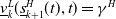


In conclusion, $(s^H, s^L, v^H, v^L)$
is a classical solution of (2.9). This completes the proof of Lemma 5.1.
$(s^H, s^L, v^H, v^L)$
is a classical solution of (2.9). This completes the proof of Lemma 5.1.
5.3. Supersolutions
For completion, here we construct a supersolution sequence. Starting from ${\bar s}_0^L(\!\cdot\!)\equiv s^L(0),$
we construct inductively
${\bar s}_0^L(\!\cdot\!)\equiv s^L(0),$
we construct inductively $\{{\bar v}_k^L,{\bar s}^H_k,{\bar v}_k^H,{\bar s}^L_{k+1}\}_{k=0}^\infty$
as follows.
$\{{\bar v}_k^L,{\bar s}^H_k,{\bar v}_k^H,{\bar s}^L_{k+1}\}_{k=0}^\infty$
as follows.
Let $k\geqslant 0$
be an integer and assume that
$k\geqslant 0$
be an integer and assume that ${\bar s}^L_k$
is known.
${\bar s}^L_k$
is known.
Step 1. We define ${\bar v}_k^L$
as the unique solution of
${\bar v}_k^L$
as the unique solution of
 \begin{eqnarray} \left \{\begin{array}{l@{\quad}l}\bar v^L_k=\gamma ^L\quad &\mbox{ for }t\gt 0,\ x\geqslant \bar s^L_k(t),\\[5pt] \min \{\mathcal{L}^L{\bar v}_{k}^L,{\bar v}_{k}^L-\gamma ^L\}=0 & \mbox{ for } t\gt 0,\ x\lt \bar s^L_k(t),\\[5pt] {\bar v}_k^L(\cdot,0)= v_0^L(\!\cdot\!) &\hbox{ on } \,{\mathbb R}. \end{array}\right . \end{eqnarray}
From the solution, we define
 \begin{eqnarray} {\bar s}_{k}^H(t)=\inf \{x|{\bar v}_{k}^L(x,t)\lt \gamma ^H\},\quad \forall \,t\geqslant 0. \end{eqnarray}
We consider two cases (1) $k=1$
(2)
$k=1$
(2) $k=0$
.
$k=0$
.
(1) Suppose $k\geqslant 1.$
We make an induction assumption that when
$k\geqslant 1.$
We make an induction assumption that when $k\geqslant 1$
,
$k\geqslant 1$
, $s^L_k\in \mathfrak{X}^L_{T^L}$
where
$s^L_k\in \mathfrak{X}^L_{T^L}$
where $\mathfrak{X}^L_{T}$
is defined in (4.1).
$\mathfrak{X}^L_{T}$
is defined in (4.1).
By Theorem 4.1, there exists a unique solution $\bar v_k^L$
to (5.11). In addition
$\bar v_k^L$
to (5.11). In addition $\bar s^H_k\in \mathfrak{X}^H_{T^H}$
, where
$\bar s^H_k\in \mathfrak{X}^H_{T^H}$
, where $\mathfrak{X}^H_{T}$
is defined in (4.2).
$\mathfrak{X}^H_{T}$
is defined in (4.2).
(2) Suppose $k=0.$
One can check that
$k=0.$
One can check that $v_k^L(\!-\!\infty,t)=e^{-\delta ^L t}\gt \gamma ^H$
for
$v_k^L(\!-\!\infty,t)=e^{-\delta ^L t}\gt \gamma ^H$
for $t\in [0, T^H).$
Still
$t\in [0, T^H).$
Still $\bar s_0^H$
is well defined and
$\bar s_0^H$
is well defined and $\bar s^H_0\in \mathfrak{X}^H_{T^H}.$
We remark that $\bar s^H_k(\!\cdot\!)\equiv -\infty \mbox{ in }[T^H,\infty ).$
Step 2. Define ${\bar v}_k^H$
as the solution of
${\bar v}_k^H$
as the solution of
 \begin{eqnarray} \left \{\begin{array}{l@{\quad}l} \mathcal{L}^H{\bar v}_{k}^H=0 & \mbox{for } x\gt{\bar s}_k^H(t),\ t\gt 0,\\[5pt] {\bar v}_k^H(x,0)= \gamma ^H\wedge e^{-x} &\hbox{for} \,x\in{\mathbb R},\ t=0, \\[5pt] {\bar v}_k^H(x,t)=\gamma ^H \quad & \mbox{for } x\leqslant{\bar s}_k^H(t),\ t\gt 0. \end{array}\right . \end{eqnarray}
Using maximum principle, we find that $0\lt \bar v_k^H\leqslant \gamma ^H.$
Thus, it is also the solution of the variational inequality
$0\lt \bar v_k^H\leqslant \gamma ^H.$
Thus, it is also the solution of the variational inequality
 \begin{equation*}\max \{\mathcal {L}^H\bar v_{k}^H,\bar v_{k}^H-\gamma ^H\}=0\quad \mbox { for } t\gt 0,\ x\gt \bar s^H_k(t).\end{equation*}
That $\bar v_k^H\leqslant \gamma ^H$
implies that
$\bar v_k^H\leqslant \gamma ^H$
implies that $\frac{\partial }{{\partial } x}\bar v^H_k(\bar s^H_k(t),t)\leqslant 0$
for
$\frac{\partial }{{\partial } x}\bar v^H_k(\bar s^H_k(t),t)\leqslant 0$
for $t\in [0,T^H).$
Thus, by the maximum principle
$t\in [0,T^H).$
Thus, by the maximum principle
 \begin{equation*}(\bar v^H_k)_x\lt 0\quad \mbox { in } \bar Q^H_k=\{(x,t)\ | \ t\gt 0,x\gt \bar s^H_k(t)\}.\end{equation*}
Now differentiating $\bar v^H_k(\bar s^H_k(t),t)=0$
and using
$\bar v^H_k(\bar s^H_k(t),t)=0$
and using $ (\bar s^H_k)'(t)\leqslant 0$
for
$ (\bar s^H_k)'(t)\leqslant 0$
for $t\in [0,T^H),$
we find that
$t\in [0,T^H),$
we find that
 \begin{equation*}(\bar v^H_k)_t\lt 0\quad \mbox { in } \bar Q^H_k. \end{equation*}
Finally, by construction sub-supersolutions (c.f. the proof of Theorem 4.1), we can show that
 \begin{equation*}\lim _{x\to -\infty }\bar v _k^H(x,t)=\Big \{\begin {array}{l@{\quad}l}\gamma ^H\quad &\mbox { if }t\in [0,T^H),\\[5pt] \gamma ^He^{\delta ^H (t-T^H)} &\mbox { if }t\gt T^H.\end {array}\end{equation*}
Now define
 \begin{equation} {\bar s}^L_{k+1}(t)\;:\!=\;\inf \{ x|{\bar v}^H_k(x,t)\leqslant \gamma ^L\}\quad \forall t\geqslant 0. \end{equation}
One can verify that ${\bar s}_{k+1}^L\in \mathfrak{X}^L_{T^L}.$
This completes the inductive construction of
${\bar s}_{k+1}^L\in \mathfrak{X}^L_{T^L}.$
This completes the inductive construction of $\{{\bar v}_k^L,{\bar s}^H_k,{\bar v}_k^H,{\bar s}^L_{k+1}\}.$
5.4. The limit of the supersolution sequence
Furthermore, we can show the following, whose proof is omitted.
Lemma 5.2.
Start from ${\bar s}_0^L(\!\cdot\!)\equiv s^L(0)$
. Define successively a sequence
${\bar s}_0^L(\!\cdot\!)\equiv s^L(0)$
. Define successively a sequence $\{{\bar v}_k^L,{\bar s}^H_k,{\bar v}^H_k,{\bar s}_{k+1}^L\}_{k=0}^\infty$
by (5.11), (5.12), (5.13), (5.14). Then, the sequence is decreasing in
$\{{\bar v}_k^L,{\bar s}^H_k,{\bar v}^H_k,{\bar s}_{k+1}^L\}_{k=0}^\infty$
by (5.11), (5.12), (5.13), (5.14). Then, the sequence is decreasing in $k$
in the sense that for each integer
$k$
in the sense that for each integer $k\geq 0,$
 \begin{eqnarray*} &{\underline{s}}^H_k(t)\leqslant{\bar s}_{k+1}^H (t)\le{\bar s}_{k} ^H(t) \le{\bar s}^L_{k+1}(t)\le{\bar s}_{k}^L(t) \leqslant s^L(0) \quad \forall \, t\gt 0, \\[5pt] &{\underline{v}}_k^H\leqslant{\bar v}_{k+1}^H \leqslant{\bar v}^H_{k}\leqslant \gamma ^H,\quad{\underline{v}}^L_k\leqslant{\bar v}_{k+1}^L \leqslant{\bar v}_{k}^L \leqslant 1\quad \hbox{ in } \,{\mathbb R}\times [0,\infty ). \end{eqnarray*}
Consequently, for each $t\geqslant 0$
and
$t\geqslant 0$
and $x\in{\mathbb R}$
, the limit
$x\in{\mathbb R}$
, the limit
 \begin{eqnarray*} \big [s^H(t),s^L(t), v^H(x,t),v^L(x,t)\big ] = \lim _{k\to \infty } \big [{\bar s}_k^H(t),{\bar s}_k^L(t),{\bar v}_k^H(x,t),{\bar v}_k^L(x,t)\big ] \end{eqnarray*}
exists and forms a solution of the free boundary problem (2.9) .
6. Main theorem and uniqueness
Now we present our main mathematical result of our paper.
Theorem 6.1 (Main theorem). The free boundary problem (2.9) admits a unique solution $(s^H,s^L,\hat{s}^L,v^H,v^L)$
. The solution satisfies
$(s^H,s^L,\hat{s}^L,v^H,v^L)$
. The solution satisfies
 \begin{eqnarray*} &&s^L\in \mathfrak{X}^L_{T^L},\quad s^H\in \mathfrak{X}^H_{T^H}, \\[5pt] && v^L \in C^1\big (\overline{Q^L}\setminus (0,0)\big )\cup C^\infty \big ({\hat{Q}^L}\cup ((\!-\!\infty,0)\cap (0,s^L(0))\times \{0\})\big ),\\[5pt] && v^H \in C^\infty \big ( \overline{Q^H}\setminus (s^H(0),0)\big ), \end{eqnarray*}
where $Q^H\;:\!=\;\{(x,t)\;|\; t\gt 0, x\gt s^H(t)\}$
,
$Q^H\;:\!=\;\{(x,t)\;|\; t\gt 0, x\gt s^H(t)\}$
, $Q^L\;:\!=\;\{(x,t)\;|\; t\gt 0,\ x\lt s^L(t)\}$
and
$Q^L\;:\!=\;\{(x,t)\;|\; t\gt 0,\ x\lt s^L(t)\}$
and $\hat{Q}^L\;:\!=\;\{(x,t)\;|\; t\gt 0,\ x\lt \hat{s}^L(t)\}$
. In addition,
$\hat{Q}^L\;:\!=\;\{(x,t)\;|\; t\gt 0,\ x\lt \hat{s}^L(t)\}$
. In addition,
 \begin{eqnarray*} &&v^H_x\lt 0,\ v^H_t \lt 0\ {\ in} \,Q^H;\quad v^L_x\lt 0,\ v^L_t \lt 0\ {\ in } \,\hat{Q}^L;\\[5pt] &&s^H\equiv -\infty \ {\ in }[T^H,\infty );\quad s^L\equiv -\infty \ {\ in }[T^L,\infty );\\[5pt] && \frac{d\hat{s}^L}{d t}\leqslant 0\ {\ in } (0,T^L);\quad{\frac{d s^H}{d t}\lt 0\ {\ in } (0,T^H);\quad \frac{d s^L}{d t}\lt 0 \ {\ in } (0,T^L);}\\[5pt] && s^L(t)-s^H(t) \gt \ln \frac{\gamma ^H}{\gamma ^L},\quad s^H(t)\lt \hat{s}^L(t)\leqslant s^L(t),\quad \hbox{for} \,t\in [0,T^H).\\[5pt] \end{eqnarray*}
Proof. The existence comes from the limit of the sequence and lemmas in Section 5.
For the uniqueness, let $(v_i^H,v_i^L,s_i^H,s_i^L)$
,
$(v_i^H,v_i^L,s_i^H,s_i^L)$
, $i=1,2$
, be two solutions of (2.9). Fix an arbitrary positive
$i=1,2$
, be two solutions of (2.9). Fix an arbitrary positive $\epsilon$
. Define
$\epsilon$
. Define $v^l_\epsilon (x,t)=v^l_2(x+\epsilon,t)$
and
$v^l_\epsilon (x,t)=v^l_2(x+\epsilon,t)$
and $s^l_\epsilon (t)=s^l_2(t)-\epsilon$
for
$s^l_\epsilon (t)=s^l_2(t)-\epsilon$
for $l=H,L.$
Define
$l=H,L.$
Define
 \begin{equation*}T_\epsilon =\sup \{t\in [0,T^H]\;|\;s_1^H(\tau )\gt s_2^H(\tau )-\epsilon \quad \forall \tau \in [0,t) \}.\end{equation*}
Clearly, from $s_1^H(0)=s_2^H(0)$
, we have
$s_1^H(0)=s_2^H(0)$
, we have $T_\epsilon \gt 0.$
By strong comparison,
$T_\epsilon \gt 0.$
By strong comparison,
 \begin{eqnarray*} v_1^H(x,t)\gt v^H_\epsilon (x,t)\quad \forall t\in [0,T_\epsilon ],\ x\gt s^H_\epsilon \;:\!=\;s_2^H(t)-\epsilon . \end{eqnarray*}
This implies $s_1^L(t)\gt s^L_\epsilon (t)$ $\forall t\in [0,T_\epsilon ].$
Now we claim that
$\forall t\in [0,T_\epsilon ].$
Now we claim that $T_\epsilon =T^H.$
In fact, supposed not, then
$T_\epsilon =T^H.$
In fact, supposed not, then
 \begin{equation*}s_1^H(T_\epsilon ) =s_2^H(T_\epsilon )-\epsilon =s^H_\epsilon (T_\epsilon ).\end{equation*}
By comparison, $v_1^L\geqslant v^L_\epsilon$
in
$v_1^L\geqslant v^L_\epsilon$
in ${\mathbb R}\times [0,T_\epsilon ]$
. It follows from strong comparison that
${\mathbb R}\times [0,T_\epsilon ]$
. It follows from strong comparison that $v_1^L\gt v^L_\epsilon$
in
$v_1^L\gt v^L_\epsilon$
in $\{(x,t)\ |\ x\lt \hat{s}^L(t),0\lt t\leqslant T_\epsilon \}.$
But this implies
$\{(x,t)\ |\ x\lt \hat{s}^L(t),0\lt t\leqslant T_\epsilon \}.$
But this implies
 \begin{eqnarray*} &&\gamma ^H=v_1^L(s^H_1(T_\epsilon ),T_\epsilon )\gt v^L_\epsilon (s^H_\epsilon (T_\epsilon ),T_\epsilon )=v_2^L(s^H_2(T_\epsilon ),T_\epsilon ))=\gamma ^H, \end{eqnarray*}
a contradiction. Thus, $T_\epsilon =T^H$
. It follows that
$T_\epsilon =T^H$
. It follows that
 \begin{eqnarray*} &&v_1^L(x,t)\gt v_2^L(x+\epsilon,t),\quad s^L_1(t)\gt s_2^L(t)-\epsilon \quad \forall t\in [0,T^H),\ x\gt s^H_1(t),\\[5pt] &&v_1^H(x,t)\gt v_2^H(x+\epsilon,t),\quad s^H_1(t)\gt s_2^H(t)-\epsilon \quad \forall t\in [0,T^H),\ x\lt s^L_1(t). \end{eqnarray*}
Sending $\epsilon \to 0,$
we have, for
$\epsilon \to 0,$
we have, for $l=H,L$
,
$l=H,L$
,
 \begin{equation*}v_1^l(x,t)\geqslant v_2^l(x,t),\quad s^l_1(t)\geqslant s^l_2(t)\qquad \forall t\in [0,T^H],\ x\in {\mathbb R}.\end{equation*}
Reversing the roles of the two solutions, we see that $v_1^H=v^H_2$
and
$v_1^H=v^H_2$
and $v_1^L=v^L_2$
in
$v_1^L=v^L_2$
in ${\mathbb R}\times [0,T^H]$
. Since
${\mathbb R}\times [0,T^H]$
. Since $\mathcal{L}^Hv_i^H=0$
in
$\mathcal{L}^Hv_i^H=0$
in ${\mathbb R}\times [T^H,\infty ),$
we have
${\mathbb R}\times [T^H,\infty ),$
we have $v^H_1=v^H_2$
in
$v^H_1=v^H_2$
in ${\mathbb R}\times [T^H,\infty ),$
which implies
${\mathbb R}\times [T^H,\infty ),$
which implies $s^L_1\equiv s^L_2$
on
$s^L_1\equiv s^L_2$
on $[T^H,T^L),$
and
$[T^H,T^L),$
and $v^L_1\equiv v^L_2$
on
$v^L_1\equiv v^L_2$
on ${\mathbb R}\times [T^H,\infty ).$
We then have proved the uniqueness.
${\mathbb R}\times [T^H,\infty ).$
We then have proved the uniqueness.
Remark 6.1. Note that $e^{-x}$
is a steady state. This implies that
$e^{-x}$
is a steady state. This implies that $\frac{{\partial }^k}{{\partial } t^k} v^H(x,0)=0$
when
$\frac{{\partial }^k}{{\partial } t^k} v^H(x,0)=0$
when $x\in (s^H(0),\infty )$
for any integer
$x\in (s^H(0),\infty )$
for any integer $k\geqslant 1.$
This further implies that
$k\geqslant 1.$
This further implies that $\frac{d^k}{d t^k} s^L(0)=0$
for any
$\frac{d^k}{d t^k} s^L(0)=0$
for any $k\geqslant 1.$
Similarly, we have
$k\geqslant 1.$
Similarly, we have $\frac{d^k}{d t^k} s^H(0)=0$
for any
$\frac{d^k}{d t^k} s^H(0)=0$
for any $k\geqslant 1.$
Remark 6.2. Note that if $\hat{s}^L(t)\lt s^L(t),$
then
$\hat{s}^L(t)\lt s^L(t),$
then $v_x^L(\hat{s}^L(t),t)=0.$
Since
$v_x^L(\hat{s}^L(t),t)=0.$
Since $v_x^L(\hat{s}^L(0)-,0)\lt 0,$
we see that there exist
$v_x^L(\hat{s}^L(0)-,0)\lt 0,$
we see that there exist $T\gt 0$
such that
$T\gt 0$
such that $\hat{s}^L(t)=s^L(t)$
for
$\hat{s}^L(t)=s^L(t)$
for $t\in [0,T].$
Remark 6.3. In the case $\delta ^L\gt \delta ^H$
, we can see clear the need of the variational inequality. First of all, we have
$\delta ^L\gt \delta ^H$
, we can see clear the need of the variational inequality. First of all, we have
 \begin{equation*}v^H(\!-\!\infty,t)=\Big \{\begin {array}{l@{\quad}l}\gamma ^H\quad &\mbox { if }\ 0\leqslant t\lt T^H,\\[5pt] \gamma ^H e^{-\delta ^H(t-T^H)}\quad &\mbox { if }\ t\geqslant T^H.\end {array}\end{equation*}
This implies, using the notation (2.8), that $s^L\in C^\infty ([0, T^L))$
. However, we know that
$s^L\in C^\infty ([0, T^L))$
. However, we know that $v^L\lt e^{-\delta ^L t}$
for
$v^L\lt e^{-\delta ^L t}$
for $t\in [0,\hat{T}^L)$
. Thus, we have
$t\in [0,\hat{T}^L)$
. Thus, we have $v^L(\cdot,t)\equiv \gamma ^L,$ $\hat{s}^L(t)=-\infty \lt s^L(t)$
for
$\hat{s}^L(t)=-\infty \lt s^L(t)$
for $t\in [\hat{T}^L, T^L).$
Therefore, we must replace the PDEs in [Reference Chen and Liang3] by variational inequalities.
$t\in [\hat{T}^L, T^L).$
Therefore, we must replace the PDEs in [Reference Chen and Liang3] by variational inequalities.
7. Summary
Mathematical analyses of credit rating migration using structure frameworks start from [Reference Liang and Zeng14], where the migration boundary is assumed to be known. The work is extended in [Reference Hu, Liang and Wu10, Reference Liang, Wu and Hu12] by assuming that the migration boundary is a free boundary determined by the equation $R=\gamma$
, where
$R=\gamma$
, where $R$
is the ratio of debt and asset value and
$R$
is the ratio of debt and asset value and $\gamma$
is a threshold. Since a Brownian motion
$\gamma$
is a threshold. Since a Brownian motion $W_t-W_{t_0}$
can change sign infinite many time in
$W_t-W_{t_0}$
can change sign infinite many time in $[t_0,t_0+\epsilon )$
for any
$[t_0,t_0+\epsilon )$
for any $\epsilon \gt 0$
, the free boundary models in [Reference Hu, Liang and Wu10, Reference Liang, Wu and Hu12] may result in the change of credit rating infinite many times in short time. Thus, for realistic application, an introduction of a buffer zone (dead band in engineering) is necessary. In our previous paper [Reference Chen and Liang3], a credit rating migration model with a buffer zone is introduced. However, we discover that the model works only for the case of nondividend. In this paper, we revise the credit rating migration model in [Reference Chen and Liang3], so that it covers the non-zero dividend case. It is not a trivial extension as the PDE problem will bring up the possibility of the solution violates the rating migration condition inside of the region; i.e. if we only use PDE, then the solution
$\epsilon \gt 0$
, the free boundary models in [Reference Hu, Liang and Wu10, Reference Liang, Wu and Hu12] may result in the change of credit rating infinite many times in short time. Thus, for realistic application, an introduction of a buffer zone (dead band in engineering) is necessary. In our previous paper [Reference Chen and Liang3], a credit rating migration model with a buffer zone is introduced. However, we discover that the model works only for the case of nondividend. In this paper, we revise the credit rating migration model in [Reference Chen and Liang3], so that it covers the non-zero dividend case. It is not a trivial extension as the PDE problem will bring up the possibility of the solution violates the rating migration condition inside of the region; i.e. if we only use PDE, then the solution $\mathcal{L}^Lv^L=0$
in
$\mathcal{L}^Lv^L=0$
in $\{(x,t)| t\in [0,T^L),x\lt s^L(t)\}$
may not satisfy the fundamental requirement that
$\{(x,t)| t\in [0,T^L),x\lt s^L(t)\}$
may not satisfy the fundamental requirement that $v^L\geqslant \gamma ^L$
, see Remark 6.3. For this reason, we modify the model by replacing the parabolic equation by a variational inequality. This renders to a new free boundary problem where the PDE free boundary problem in [Reference Chen and Liang3] is a special case of the new model. By constructing two monotone sequences, existence, uniqueness and some properties are obtained.
$v^L\geqslant \gamma ^L$
, see Remark 6.3. For this reason, we modify the model by replacing the parabolic equation by a variational inequality. This renders to a new free boundary problem where the PDE free boundary problem in [Reference Chen and Liang3] is a special case of the new model. By constructing two monotone sequences, existence, uniqueness and some properties are obtained.
The model established in this paper can be extended without essential difficulties to the cases of multiple ratings. It can be expected to be used by credit rating companies, bond issuing agencies and corresponding financial institutions.
Financial support
This work was supported by the National Natural Science Foundation of China 12071349.
Competing interests
None.


 Open access