


1. Introduction
Precision agriculture technology is currently available to apply different levels of fertilizer across a field. Multiple firms such as the Climate Corporation™ have been created to guide producers in choosing fertilizer rates and making other decisions. Precision nitrogen fertilizer applications, however, have not been widely adopted. Presumably, this is due to the available agricultural economics and agronomic research being not yet sufficient to make it profitable. To make precision nitrogen application profitable, it may require gathering information from multiple sources. The question addressed here is how to make better use of historical yield-monitor data that were based on uniform rate applications. Yield-monitor data are already widely available and so these data are a potential low-cost source of information. The problem is that most historical yield-monitor data are based on using the same nitrogen rate across the whole field, which makes it difficult to estimate a production function with different parameters for each site. The solution proposed here is to use Bayesian Kriging to estimate a linear plateau model where the plateau is the only parameter that varies across the field. Bayesian Kriging works because it uses information from nearby plots to estimate the plateau parameters.
Considerable research has used spatial data to estimate yield response to nitrogen, such as by using spatial error models (Anselin et al., Reference Anselin, Bongiovanni and Lowenberg-DeBoer2004), but such models do not have spatially varying coefficients. To allow parameters to vary across space, past studies seeking site-specific recommendations defined subareas of the field and used dummy variables to allow expectations to spatially vary across the subareas (Hurley et al., Reference Hurley, Malzer and Killian2004; Lambert et al., Reference Lambert, Lowenberg-DeBoer and Bongiovanni2004; Lambert et al., Reference Lambert, Lowenberg-DeBoer and Malzer2006; Liu et al., Reference Liu, Swinton and Miller2006). The arbitrarily defined subarea dummies are likely less precise than letting the model select the spatial relationships. The dummy-variable also does not allow defining the causality of the site heterogeneity as a function of distance, which could be measured as Euclidean distance, soil type similarity, or elevation. The dummy variable approach does not allow response coefficients to vary smoothly across the field, either. Further, these past studies required on-farm experiment data where nitrogen was varied randomly over the field. But in practice, most historical yield data will be from fields where a uniform rate was applied on the entire field.
If enough years of data were available, input response coefficients for every site could be obtained with separate regressions for each site. For instance, if there are N sites, then N separate regressions would be needed with each using only one site’s observation. Most available time series are too short to accurately estimate site-specific parameters in this way. The geographically weighted regression (GWR) models of Lambert and Cho (Reference Lambert and Cho2022) and Trevisan et al. (Reference Trevisan, Bullock and Martin2021) can estimate spatially varying coefficients, but they cannot consider the case of uniform nitrogen rates. In most cases, producers will have informative priors and limited data, so the Bayesian approach offers potential advantages in precision over GWR.
Note that machine learning methods that have proven successful in predicting both yield (Ruan et al., Reference Ruan, Li, Yuan, Cammarano, Ata-Ul-Karim, Li, Tian, Zhu, Cao and Cao2022) and nitrogen response (Kakimoto et al., Reference Kakimoto, Mieno, Tanaka and Bullock2022) do not have spatially varying coefficients. With a spatially varying coefficient model, there will be few observations at each location and the restrictions provided by a parametric model are necessary to make the model estimable.
The new method is illustrated using five years of data collected from continuous corn production in Mississippi. Yield data were obtained from a high-resolution yield monitor and were aggregated to a grid with 100 × 100-m cells. A linear stochastic plateau production function was used as in Tembo et al. (Reference Tembo, Brorsen, Epplin and Tostão2008) to estimate a different plateau for each cell. The other parameters were not spatially varying.
2. Bayesian modeling framework
2.1. Crop response function
Past research on crop yield response to nitrogen fertilizer used a variety of functional forms (Dhakal and Lange, Reference Dhakal and Lange2021; Miguez and Poffenbarger, Reference Miguez and Poffenbarger2022). Many of them such as Nafziger and Rapp (Reference Nafziger and Rapp2021) use various forms of plateau models. Plateaus can potentially vary across locations and years. The stochastic linear response plateau function (Tembo et al., Reference Tembo, Brorsen, Epplin and Tostão2008) lets the plateau vary across time, but not space. Stochastic plateau models with year-random effects have been estimated with both classical (Dhakal et al., Reference Dhakal, Lange, Parajulee and Segarra2019; Tembo et al., Reference Tembo, Brorsen, Epplin and Tostão2008) and Bayesian econometric methods (Ouedraogo and Brorsen, Reference Ouedraogo and Brorsen2018). Table 1 summarizes the methods used in a subset of the related literature. The research is innovative in two ways. First, it is the only one of the studies that has both stochastic time-varying parameters and spatially varying coefficients. Most importantly, it is the only model that can produce spatially varying coefficients from a field where a uniform rate was applied. The plateau is the only spatially varying coefficient, which means that each cell has its own plateau. Thus, the plateau P i at location i is spatially correlated and varies across locations within the field. With a linear plateau model, each parameter has its own individual interpretation, so it is more plausible to have some parameters vary across space and not others than it would be if a quadratic plateau model were used (with a quadratic plateau, differentiability is imposed at the switch point and so changing the plateau changes the other parameters). The model assumes uniform nitrogen input data, a linear response, and normality. The proposed site-specific stochastic plateau function can be defined as
Table 1. Summary of methods used in the current study and in previous research

Note: LRSP = Linear response stochastic plateau; LRP = Linear response plateau; SR = Switching regression; QRP = Quadratic response plateau; QRSP = Quadratic response stochastic plateau; ANOVA = analysis of variance (dummy variables); GWR = Geographically weighted regression; SRP = Switching regression plateau; NME = Nonlinear mixed-effects estimation; MLE = Maximum likelihood estimation.
 $${y_{kt}} = \min \left( {\alpha + \beta {N_t},{P_k} + {v_t}} \right) + {u_t} + {\varepsilon _{kt}}$$
where N
t
and y
kt
are the nitrogen input and response yield on the kth cell in year t, k = 1, …, K and t = 1, …, T, the plateau follows a multivariate Gaussian spatial processFootnote
1
, ${\boldsymbol{P}}\sim MVGP(\overline{\boldsymbol{{P}}}, \Sigma )$
, where
${\boldsymbol{P}}\sim MVGP(\overline{\boldsymbol{{P}}}, \Sigma )$
, where $\boldsymbol{P}=[\boldsymbol{P_{1}},\ldots, \boldsymbol{P_{K}}]'$
,
$\boldsymbol{P}=[\boldsymbol{P_{1}},\ldots, \boldsymbol{P_{K}}]'$
, $\overline{\boldsymbol{{P}}}$
is a
$\overline{\boldsymbol{{P}}}$
is a $K\times 1$
vector of the mean plateau across all locations, where
$K\times 1$
vector of the mean plateau across all locations, where $\overline{\boldsymbol{{P}}}=[\overline{P},\ldots, \overline{P}]'$
and an exponential spatial covariance function was assumed so
$\overline{\boldsymbol{{P}}}=[\overline{P},\ldots, \overline{P}]'$
and an exponential spatial covariance function was assumed so $\Sigma _{kj}=\rho e^{{-D_{kj}}/\theta }$
where
$\Sigma _{kj}=\rho e^{{-D_{kj}}/\theta }$
where $D_{kj}$
is distance,
$D_{kj}$
is distance, $v_{t}$
and
$v_{t}$
and $u_{t}$
are plateau and intercept year-random effects that were assumed to follow
$u_{t}$
are plateau and intercept year-random effects that were assumed to follow $v_{t}\sim N(0, \sigma _{v}^{2})$
and
$v_{t}\sim N(0, \sigma _{v}^{2})$
and $u_{t}\sim N(0, \sigma _{u}^{2})$
, respectively, and
$u_{t}\sim N(0, \sigma _{u}^{2})$
, respectively, and $\varepsilon _{kt}$
is an independently identically distributed error
$\varepsilon _{kt}$
is an independently identically distributed error $\varepsilon _{it}\sim N(0, \sigma ^{2})$
. As discussed in Tembo et al., (Reference Tembo, Brorsen, Epplin and Tostão2008, p. 426), the specification in (1) can equivalently be written as having intercept and plateau random effects with a restriction on the covariance of the two effects. The space and time effects are independent here. Wikle et al., (Reference Wikle, Zammit-Mangion and Cressie2019) discuss spatio-temporal models where space and time effects interact, but the data used here are insufficient to estimate such a model.
$\varepsilon _{it}\sim N(0, \sigma ^{2})$
. As discussed in Tembo et al., (Reference Tembo, Brorsen, Epplin and Tostão2008, p. 426), the specification in (1) can equivalently be written as having intercept and plateau random effects with a restriction on the covariance of the two effects. The space and time effects are independent here. Wikle et al., (Reference Wikle, Zammit-Mangion and Cressie2019) discuss spatio-temporal models where space and time effects interact, but the data used here are insufficient to estimate such a model.
Intuitively, $\boldsymbol{{P}}$
was modeled as a deterministic constant
$\boldsymbol{{P}}$
was modeled as a deterministic constant $\overline{\boldsymbol{{P}}}$
plus a spatial random effectFootnote
2
. Each spatial random effect is estimated rather than estimating its variance so the effects are included when obtaining expected yields.
$\overline{\boldsymbol{{P}}}$
plus a spatial random effectFootnote
2
. Each spatial random effect is estimated rather than estimating its variance so the effects are included when obtaining expected yields.
An important point here is modeling the input response: $\mu _{t}=\alpha +\beta N_{t}$
. Most yield-monitor data, including the data used here, are based on uniform nitrogen applications. Since the nitrogen applied did not vary, there is limited information to estimate parameters
$\mu _{t}=\alpha +\beta N_{t}$
. Most yield-monitor data, including the data used here, are based on uniform nitrogen applications. Since the nitrogen applied did not vary, there is limited information to estimate parameters $\alpha$
and
$\alpha$
and $\beta$
(they could not be estimated with a single year of data). Therefore, instead of estimating the response coefficients,
$\beta$
(they could not be estimated with a single year of data). Therefore, instead of estimating the response coefficients, $\mu _{t}$
was interpreted as the uniform target yield, say
$\mu _{t}$
was interpreted as the uniform target yield, say $\mu$
, to reflect the empirical dataset with uniform nitrogen availableFootnote
3
, say Ñ.
$\mu$
, to reflect the empirical dataset with uniform nitrogen availableFootnote
3
, say Ñ.
In terms of Bayesian thinking, there would be uncertainty about the intercept (α) and the slope (β) parameters. As discussed by Liu et al. (Reference Liu, Swinton and Miller2006), there might also be a year-to-year variation in the target yield due to variations in nitrogen available from natural sources. To address these uncertainties, an informative prior was imposed on the μ. Year-to-year variation was included and thus target yield μ t varied by year.
2.2. Hierarchical structure
As in Park et al. (Reference Park, Brorsen and Harri2019), the proposed Bayesian Kriging approach has three hierarchical layers, which are the likelihood layer, process layer, and prior layer. First, in the likelihood layer, crop yields are assumed normally distributed conditional on the spatial and year-random effects. Second, the process layer models the distribution of the spatial random effects and the spatial structure of their density. The third layer contains the priors for all parameters.
Let
Y
denote a K × T matrix of actual crop yield observations that includes all sites and years, which is assumed to follow a conditional Gaussian distribution. Also, the error term
ε
t
is assumed to be independently normally distributed $N({\bf 0}, \sigma ^{2}\boldsymbol{{I}})$
, where σ
2 is the independently identically distributed pure error variance and
I
is an K × K identity matrix.
$N({\bf 0}, \sigma ^{2}\boldsymbol{{I}})$
, where σ
2 is the independently identically distributed pure error variance and
I
is an K × K identity matrix.
To define the layers of the hierarchical model, it is helpful to define three sets of parameters. First, are the parameters used in the likelihood layer but not drawn through the process layer, ${\bf \Theta}_{1}=$
[μ
t
, σ
v
2, σ
u
2, σ
2]′. Second, are the spatially smoothed site-specific plateau parameters
${\bf \Theta}_{1}=$
[μ
t
, σ
v
2, σ
u
2, σ
2]′. Second, are the spatially smoothed site-specific plateau parameters ${\bf \Theta}_{2}$
= (
P
) that are used in the likelihood layer but drawn through the process layer. Third, are the parameters that determine the distribution of
P
through the process layer, also known as hyper parameters,
${\bf \Theta}_{2}$
= (
P
) that are used in the likelihood layer but drawn through the process layer. Third, are the parameters that determine the distribution of
P
through the process layer, also known as hyper parameters, ${\bf \Theta}_{3}=[\rho,\theta ]'$
. The hierarchy is thus
${\bf \Theta}_{3}=[\rho,\theta ]'$
. The hierarchy is thus
 $$ \boldsymbol{{Y}}|{\bf \Theta}_{\rm 1},{\bf \Theta}_{\rm 2},{\bf \Theta}_{\rm 3}\sim {\it f_{Y}}\left(\boldsymbol{{Y}}| {\bf \Theta}_{\rm 1},{\bf \Theta}_{\rm 2}\right) $$
 $$ {\bf \Theta}_{{\rm 2}}|{\bf \Theta}_{{\rm 3}}\sim f_{{{\bf \Theta}_{{\rm 2}}}}\left({\bf \Theta}_{{\rm 2}}|{\bf \Theta}_{{\rm 3}}\right) $$
 $${\bf \Theta}_{{\rm 1}}\sim f_{1}\left({\bf \Theta}_{{\rm 1}}\right)\ {\rm and}\ {\bf \Theta}_{\rm 3}\sim {\it f}_{3}\left({\bf \Theta}_{\rm 3}\right)$$
where f() are the densities associated with each layer of the hierarchy, likelihood layer, process layer, and prior layer, Y is a K × T matrix of crop yield observations.
By Bayes’ theorem, the posterior distribution of the model is
 $$f\left( {\bf \Theta}_{1},{\bf \Theta}_{2},{\bf \Theta}_{3}|\boldsymbol{{Y}}\right)\propto f_{Y}\left(\boldsymbol{{Y}}| {\bf \Theta}_{\rm 1},{\bf \Theta}_{\rm 2}\right)\times f_{{{\bf \Theta}_{{\bf 2}}}}\left({\bf \Theta}_{{\rm 2}}\right| {\bf \Theta}_{{\rm 3}})\times f_{3}({\bf \Theta}_{3})\times f_{1}({\bf \Theta}_{{\rm 1}})$$
Therefore, the joint posterior density of the model $f({\bf \Theta}_{1},{\bf \Theta}_{2},{\bf \Theta}_{3}|\boldsymbol{{Y}})$
is proportional to the multiplication of the three layers, which are specified in the following subsections.
$f({\bf \Theta}_{1},{\bf \Theta}_{2},{\bf \Theta}_{3}|\boldsymbol{{Y}})$
is proportional to the multiplication of the three layers, which are specified in the following subsections.
2.2.1. Likelihood layer
A likelihood function of the crop yield forms the first layer of the model. Let y t be a vector of crop yield at year t that spans all locations, y t = [y 1t ,…,y Kt ]′. Since the model assumes conditional normality of crop yield distributions, the first layer of the model in equation (2) is
 $$f_{Y}\left({\boldsymbol{{Y}}}| {\bf \Theta}_{1},{\bf \Theta}_{2}\right)=\prod _{t=1}^{T}{1 \over \sqrt{2\pi \left| {\bf \Lambda}_{t}\right| }}\exp {\left({\boldsymbol{y}}_{t}-{\boldsymbol{\mu }}_{t}\right)'{\bf \Psi}{\bf \Lambda}_{t}^{-{\bf 1}}\left({\boldsymbol{y}}_{t}-{\boldsymbol{\mu }}_{t}\right)+\left({\boldsymbol{y}}_{t}-\boldsymbol{{P}}\right)'\left({\bf I}-{\bf \Psi}\right){\bf \Lambda}_{t}^{-{\bf 1}}\left({\boldsymbol{y}}_{t}-\boldsymbol{{P}}\right) \over 2}$$
where
Y
is a matrix of historical yield outcomes spanning all locations and years,
Y
= [
y
1,…,
y
T
],
μ
t
is a K × 1 vector of uniform target yields at year t,
μ
t
= [μ
t
,…, μ
t
]′,
P
is a vector of site-specific plateau, ${\bf \Psi}$
is a K × K diagonal matrix where the ith diagonal elements are 1 if μ < P
k
, 0 otherwise,
I
is an K × K identity matrix,
${\bf \Psi}$
is a K × K diagonal matrix where the ith diagonal elements are 1 if μ < P
k
, 0 otherwise,
I
is an K × K identity matrix, ${\bf \Lambda}_{t}$
is a K × K variance-covariance matrix,
${\bf \Lambda}_{t}$
is a K × K variance-covariance matrix, ${\bf \Lambda}_{t}=\sigma _{u}^{2}{\boldsymbol{{J}}_{t}}+\sigma ^{2}\boldsymbol{{I}}$
, that spans all locations, where
J
t
is a matrix of ones. Yang (Reference Yang2022) reviews the theoretical literature on broken-stick regressions. While there have been proofs of consistency for many different estimators, we are not aware of a formal proof of consistency of the Bayesian estimator for this model.
${\bf \Lambda}_{t}=\sigma _{u}^{2}{\boldsymbol{{J}}_{t}}+\sigma ^{2}\boldsymbol{{I}}$
, that spans all locations, where
J
t
is a matrix of ones. Yang (Reference Yang2022) reviews the theoretical literature on broken-stick regressions. While there have been proofs of consistency for many different estimators, we are not aware of a formal proof of consistency of the Bayesian estimator for this model.
2.2.2. Process layer
The process layer is the key part of the model. The process layer models spatial structure of the site-specific estimates. The spatial structure is determined by the Kriging parameters (range θ and sill ρ) and Euclidean distances (D ij ) among locations,Footnote 4 which are contained in the variance matrices Σ.
The stochastic spatial process in the model ( P ) is defined in the process layer of the model. The density is defined as the multivariate spatial stochastic processes such that
 $$f_{{{\bf \Theta}_{{\bf 2}}}}\left({\bf \Theta}_{2}\right| {\bf \Theta}_{3})={1 \over \sqrt{\left(2\pi \right)^{K}\left| \Sigma \right| }}\exp \left[-{1 \over 2}\left(\boldsymbol{{P}}-\overline{\boldsymbol{{P}}}\right)'\Sigma ^{-1}\left(\boldsymbol{{P}}-\overline{\boldsymbol{{P}}}\right)\right]$$
where $\overline{\boldsymbol{{P}}}=[\overline{P},\ldots, \overline{P}]'$
and Σ is a K × K spatial covariance matrix cov
$\overline{\boldsymbol{{P}}}=[\overline{P},\ldots, \overline{P}]'$
and Σ is a K × K spatial covariance matrix cov
 $$({P_i},{P_j}) = \sum = \rho \left[ {\matrix{
1 & {} & {{e^{ - {D_{1K}}/\theta }}} \cr
\vdots & \ddots & \vdots \cr
{{e^{ - {D_{K1}}/\theta }}} & {} & 1 \cr } } \right]$$
.
$$({P_i},{P_j}) = \sum = \rho \left[ {\matrix{
1 & {} & {{e^{ - {D_{1K}}/\theta }}} \cr
\vdots & \ddots & \vdots \cr
{{e^{ - {D_{K1}}/\theta }}} & {} & 1 \cr } } \right]$$
.
The plateau mean vector was $\overline{\boldsymbol{{P}}}=247.8$
based on the mean of historical maximum yields across all cells in the dataset (i.e., 247.8 bushels/acre). The site-specific plateau
P
has a hierarchical form and the spatial covariance Σ. In the estimation,
P
was conditionally drawn from the hyper priors of
$\overline{\boldsymbol{{P}}}=247.8$
based on the mean of historical maximum yields across all cells in the dataset (i.e., 247.8 bushels/acre). The site-specific plateau
P
has a hierarchical form and the spatial covariance Σ. In the estimation,
P
was conditionally drawn from the hyper priors of ${\bf \Theta}_{3}$
, which are sill (ρ) and range (θ).
${\bf \Theta}_{3}$
, which are sill (ρ) and range (θ).
2.2.3. Prior layer
The prior layer contains the priors for all parameters. The priors were assumed independent. Therefore, a multiplication of all priors for the parameters forms the prior layer.
Weakly informative gamma priors were used for the random effects as well as the i.i.d error based on the standard deviation of yields over five years: σ
v
, σ
u
, σ ∼ Gamma(1, 0.2). For the sill (ρ) and range (θ) parameters in the set of hyper-parameters ${\bf \Theta}_{3}$
, which describe the magnitude and length of spatial correlation among the location-specific plateau
P
, more informative priors must be imposed. Bayesian statistics literature (Banerjee, Carlin, and Gelfand, Reference Banerjee, Carlin and Gelfand2004; Cooley, Nychka, and Naveau, Reference Cooley, Nychka and Naveau2007) argues that improper priors induce improper posteriors. Therefore, the informative gamma prior for the sill was ρ ∼ Gamma(2, 0.25), based on the standard deviation of maximum yields of each cell. For the range parameter θ, the locational information (maximum distance among locations) was used to impose a prior since the range parameter could neither fall below zero nor exceed the maximum distance in the dataset. The uniform prior was θ ∼ U(0,max(D
ij
)), where max (D
ij
) is the maximum distance among locations.
${\bf \Theta}_{3}$
, which describe the magnitude and length of spatial correlation among the location-specific plateau
P
, more informative priors must be imposed. Bayesian statistics literature (Banerjee, Carlin, and Gelfand, Reference Banerjee, Carlin and Gelfand2004; Cooley, Nychka, and Naveau, Reference Cooley, Nychka and Naveau2007) argues that improper priors induce improper posteriors. Therefore, the informative gamma prior for the sill was ρ ∼ Gamma(2, 0.25), based on the standard deviation of maximum yields of each cell. For the range parameter θ, the locational information (maximum distance among locations) was used to impose a prior since the range parameter could neither fall below zero nor exceed the maximum distance in the dataset. The uniform prior was θ ∼ U(0,max(D
ij
)), where max (D
ij
) is the maximum distance among locations.
An informative normal prior was used for the target yield (bushels/acre) at μ t ∼ N(259.59, 56.25) to allow variation of the target yield associated with the parameter uncertainty of the intercept α and the response parameter β as well as year-to-year yield variation. The mean target yield of 259.59 is calculated as 120% of the historical average yield of the dataset (214.8 bushels/acre). The variance of the prior of 56.25 was calculated using the standard errors of the intercept and nitrogen response parameters in Boyer et al. (Reference Boyer, Larson, Roberts, McClure, Tyler and Zhou2013).Footnote 5 The estimated standard error of α was 3.56 and β was 0.04 and the variance of the target yield was calculated from the standard errors and the mean values of α and β.Footnote 6
The third layer in equation (2) was then a multiplication of the two sets of priors:
 $$f_{1}({\bf \Theta}_{1})\times f_{3}({\bf \Theta}_{3})=f_{\rho }\left(\rho \right)f_{\theta }\left(\theta \right)f_{\mu }\left(\mu _{t}\right)f_{v}\left(\sigma _{v}^{2}\right)f_{u}\left(\sigma _{u}^{2}\right)f_{\sigma }\left(\sigma ^{2}\right)$$
3. Data and estimation procedure
3.1. Yield-monitor data
Five years of yield-monitor data were obtained from a 224-acre corn production field between 2012 and 2016 from a collaborating farm located in the Mississippi Delta region (around 33°10’N, 90°16’W). The soil types of the field were predominantly Dubbs silt loam and Dundee silt loam, with a small portion covered by Dundee silty clay loam. The land slopes range from 0 to 2%. The field is relatively uniform and thus may not benefit from precision applications as much as a field with more variation in soil type and slope.
Continuous corn was planted for the five years of the study (2012–2016). Corn was usually planted between March 26 and April 4. Conventional tillage was used each year. A few different varieties were planted but the yield differences were minor, and therefore no variety effects were considered. In all years the field was managed with uniformly applied inputs at field level (or a large part of the field), but the input rates changed across years based on soil tests. The nitrogen fertilizers included 28–0–0–5, 300–0–2, and 32–0–0. Nitrogen was applied with a split pattern, with starters usually applied at planting (March 26 to April 4), and side-dress applied in early May (May 1 to May 5). Although it is well recognized that the timing of nitrogen fertilizer application can impact corn yield, especially in a warm and wet region like Mississippi, the timing effect is quite complex and is still an ongoing research subject without a consensus conclusion. This analysis focused only on the effect of total nitrogen and the timing effect was left for future research.
Corn yield data were collected by the John Deere GreenStar (Deere and Company, Moline, IL) grain yield monitoring system. Harvest dates ranged from August 1 to 23, depending on the year. Yield-monitor data require cleaning to remove anomalies. The yield points within 65.6 feet (20 m) of the field edge were discarded to remove abnormal yield values generated due to the turning and changing speed of the harvester. Speed anomalies (<1.4 mile/hour and >6.8 mile/hour) were also discarded. All yield values were adjusted to a moisture level of 15.5%. Finally, yield outliers (<50 bushels/acre and >300 bushels/acre) were removed. The cleaned yield-monitor data were then aggregated into squares of 100 m by 100 m, or 2.5 acres (the number of cells was limited to reduce computational time). After removing missing data, the balanced panel dataset had 112 yield cells covering five years (2012–2016). The gridded yield maps for the five years are presented in Figure 1.
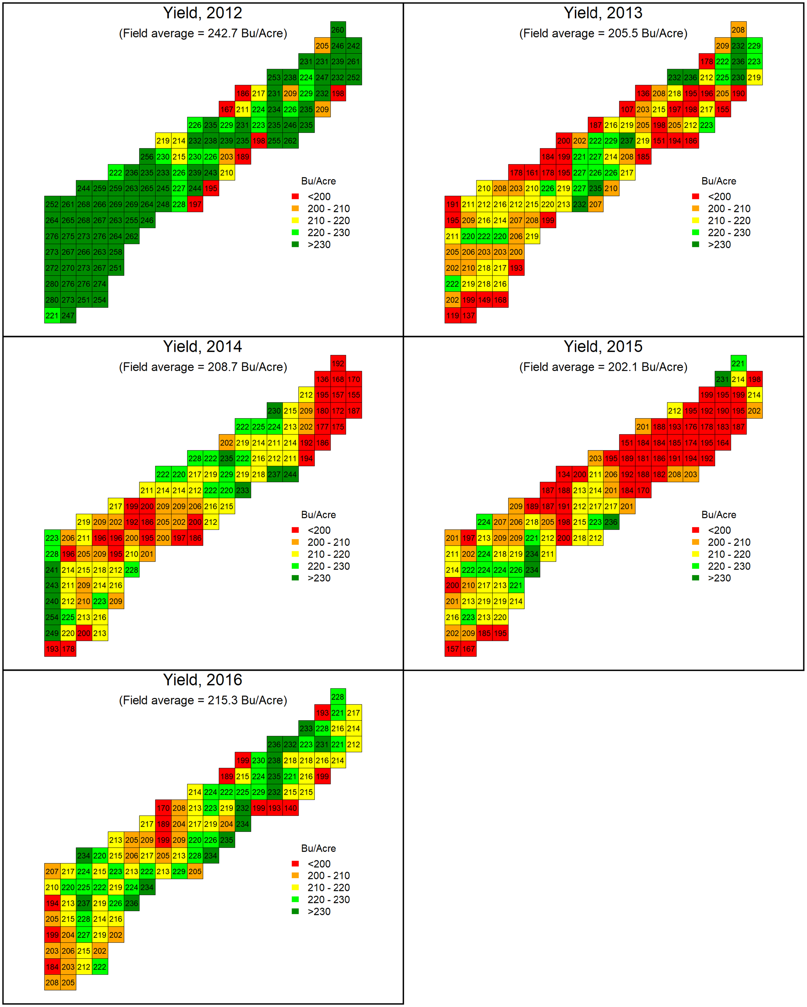
Figure 1. Mapping of cell-level (2.5-acre) corn yield by year.
The annual average yield for the study field was relatively stable over time, ranging from 202.1 bushels/acre (in 2015) to 242.7 bushels/acre (in 2012) (see Fig 1). The spatial pattern of yield variability was, however, more unstable over time. As revealed in Fig. 1, the high-yielding and low-yielding cells changed over the years. Especially in the years 2013, 2014, and 2015 when the field-average yields were similar, the spatial distributions of the yields vary substantially. But on the other hand, it is worthwhile to notice that this field’s spatial yield variation was not large. The standard deviation of cell-level yields was generally small each year, from 14.5 bushels/acre in 2016 to 23.9 bushels/acre in 2012.
3.2. Estimation
The estimation used the Hamiltonian Monte Carlo (HMC) algorithm supported by RStan (R Core Team 2018; Ng’ombe and Lambert, Reference Ng’ombe and Lambert2021; Stan Development Team, 2018). The HMC algorithm is a Markov Chain Monte Carlo method that uses Hamiltonian dynamics, and thus often needs fewer iterations to approach convergence than the Metropolis-Hastings algorithm (Jiang and Carter Reference Jiang and Carter2019). Therefore, it reduces computational time as well as failures to converge. HMC chains were run for 20,000 iterations and burn-in for 10,000. The Markov chain convergence was monitored using traceplots and Geweke (Reference Geweke1992) convergence diagnostic, which are based on a test for equality of the means of the first 10% and last 50% part of a Markov chain. The estimated parameters satisfied the convergence criteria.
Table 2 presents the estimation results of the model. The model allows the plateau P k varying over space and being site-specific. The sill (ρ) and range (θ) parameters determine the spatial structure of the plateau P k . The sill represents the magnitude of the spatial dependence among the plateau P k over space, and the range parameter represents the maximum distance of the spatial correlation among P k . The standardized distance of 0.45 for the range (θ) translates to approximately 820 feet (250 m), which means that the spatial dependence of the P k reached 820 feet. Noticeable year-to-year variations are also shown in the plateau, intercept, and the target yield.
Table 2. Estimated production function for a Mississippi delta corn field
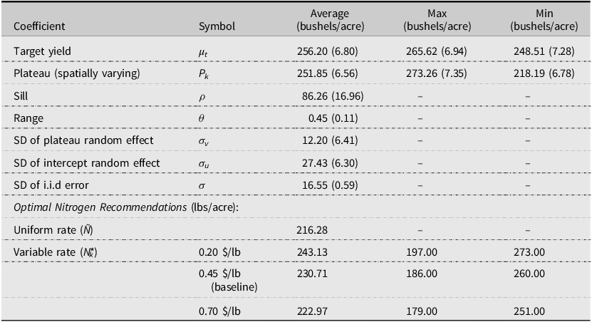
Note: The estimates are posterior means with standard deviations of posteriors in parentheses.
The posterior means of the plateaus P k were smaller than the uniform target yield at μ = 259.59 bushels/acre, as expected. The plateaus show considerable spatial variations. As stated in endnote 3, the model was also estimated under the different target yield priors of the lower (110%), baseline (120%), and upper priors (130% of the historical average yield) to verify the robustness of the plateau estimates. Regardless of the target yield prior selections, all the maps in Figure 2 present similar plateau estimates. The upper-right side of the field in Figure 2 (for all the lower, baseline, and upper target yield priors) shows lower plateaus and the lower-left side of the field shows higher-plateau estimates. The highest and the lowest plateaus were 278.26 bushels/acre and 218.19 bushels/acre.
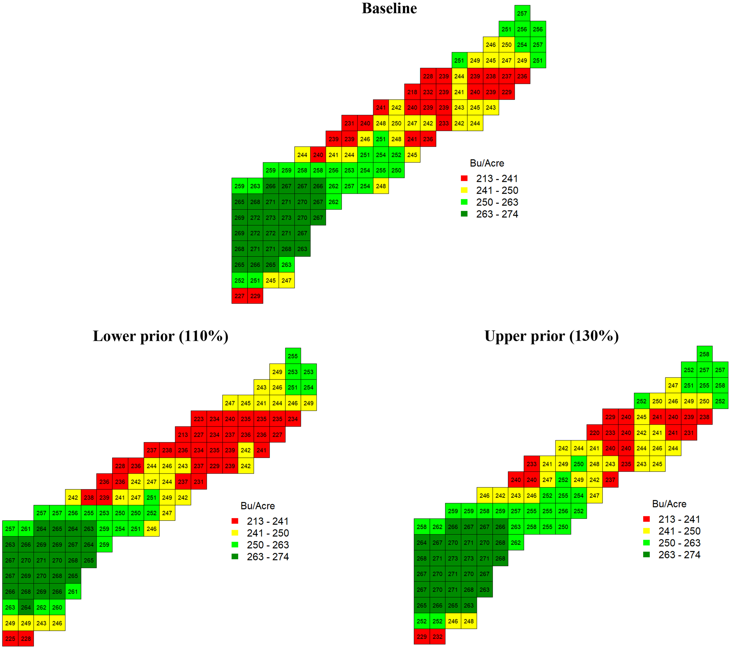
Figure 2. Estimated plateau for each cell.
3.3. Optimal nitrogen level recommendation
Assuming all other inputs predetermined, the optimal level of input N k can be determined for each location k by maximizing the net return to nitrogen:
 $$ \max _{N_{k}} E\left(\pi _{k}|N_{k}\right)=\int \left[RE\left(y\left(N_{k};{\boldsymbol{\Psi}}\right)\right)-rN_{k}\right]\ f_{{\boldsymbol{ \Psi}}}\left({\boldsymbol{\Psi}}\right)\boldsymbol{{d}}{\boldsymbol{\Psi}} $$
subject to
 $$E(y\left(N_{k};\boldsymbol{{\Psi}}\right)) = E[\min \left(\alpha +\beta N_{k},P_{k}+v_{t}\right)]$$
where ${\boldsymbol{\Psi}} =\{\alpha, \beta, P_k, \sigma_v\}, f_{\boldsymbol{\Psi}}(\boldsymbol{\Psi})$
is a set of posterior/probability distributions of
${\boldsymbol{\Psi}} =\{\alpha, \beta, P_k, \sigma_v\}, f_{\boldsymbol{\Psi}}(\boldsymbol{\Psi})$
is a set of posterior/probability distributions of $\boldsymbol{\Psi}$
, R is a corn price, and r is a nitrogen price. Both P
k
and σ
v
have numerical posteriors that were generated from the Bayesian estimation procedure. Hence, the proposed approach is akin to Ouedraogo and Brorsen (Reference Ouedraogo and Brorsen2018). McFadden, Brorsen, and Raun (Reference McFadden, Brorsen and Raun2018) did not use Bayesian estimation and calculated their posteriors with an analytical approximation.
$\boldsymbol{\Psi}$
, R is a corn price, and r is a nitrogen price. Both P
k
and σ
v
have numerical posteriors that were generated from the Bayesian estimation procedure. Hence, the proposed approach is akin to Ouedraogo and Brorsen (Reference Ouedraogo and Brorsen2018). McFadden, Brorsen, and Raun (Reference McFadden, Brorsen and Raun2018) did not use Bayesian estimation and calculated their posteriors with an analytical approximation.
The Tembo et al. (Reference Tembo, Brorsen, Epplin and Tostão2008) plug-in method to determine the optimal level of input is
 $$N_{k}^{*}={1 \over \beta }\left[P_{k}+\sigma _{v}\Phi ^{-1}\left(1-{r \over R\beta }\right)-\alpha \right]$$
where R is corn price, r is nitrogen price, and Φ is cumulative density function of the standard normal distribution. For commercial applications, the Tembo et al. (Reference Tembo, Brorsen, Epplin and Tostão2008) approach might be accurate enough where average posterior means of P k and σ v were plugged into (8).
To obtain the optimal nitrogen recommendations ${N_k^*}$
, a grid search was used rather than the plug-in method. The method used the posteriors of the estimated parameters P
k
and σ
v
. Additionally, the uncertainty of intercept (α) and nitrogen response parameters (β) was considered under a normality assumption. The optimal nitrogen level
${N_k^*}$
, a grid search was used rather than the plug-in method. The method used the posteriors of the estimated parameters P
k
and σ
v
. Additionally, the uncertainty of intercept (α) and nitrogen response parameters (β) was considered under a normality assumption. The optimal nitrogen level ${N_k^*}$
was obtained from the following maximization problem:
${N_k^*}$
was obtained from the following maximization problem:
 $$ \underset{N_{k}\in S}{{\rm argmax}}\ E\left(\pi _{k}|N_{k}\right)=\int \left[RE\left(y\left(N_{k};\boldsymbol{\Psi}\right)\right)-rN_{k}\right]f_{\boldsymbol{\Psi}}\left(\boldsymbol{\Psi}\right)\boldsymbol{d}\boldsymbol{{\Psi}} $$
subject to
 $$S=\left\{0,1,\ldots,499,500\right\}$$
where $f_{\boldsymbol{\Psi}}(\boldsymbol{\Psi})$
is a set of probability (posterior) distributions of
$f_{\boldsymbol{\Psi}}(\boldsymbol{\Psi})$
is a set of probability (posterior) distributions of $\boldsymbol{\Psi}$
= {α, β, P
i
, σ
v
}.
$\boldsymbol{\Psi}$
= {α, β, P
i
, σ
v
}.
The Monte Carlo integration requires generating samples of α and β. The priors based on Boyer et al. (Reference Boyer, Larson, Roberts, McClure, Tyler and Zhou2013) were α ∼ N(93.21, 3.562) and $\beta \sim N\left({1 \over 1.3}, 0.04^{2}\right)$
.Using 10,000 samples for each parameter, the net return values for each cell (N
k
∈ S) were calculated. Since there were 10,000 posterior pairs (as well as samples of α and β) and the plateau year-random effect term (u
t
) for 5 years, there were 50,000 net return values for each cell. These net return values were averaged for each cell. The grid-search method finds the N
k
that maximizes the average net return, say
$\beta \sim N\left({1 \over 1.3}, 0.04^{2}\right)$
.Using 10,000 samples for each parameter, the net return values for each cell (N
k
∈ S) were calculated. Since there were 10,000 posterior pairs (as well as samples of α and β) and the plateau year-random effect term (u
t
) for 5 years, there were 50,000 net return values for each cell. These net return values were averaged for each cell. The grid-search method finds the N
k
that maximizes the average net return, say ${N_k^*}$
. This process was repeated for all 112 locations.
${N_k^*}$
. This process was repeated for all 112 locations.
The optimal nitrogen recommendations were determined under three different input prices. The baseline scenario used an average corn futures price (Chicago Mercantile Exchange) and an average nitrogen price of 2016 (Schnitkey, Reference Schnitkey2016). Hence, R = 3.61 ($/bushel) and r = 0.45 ($/lb). In the two other scenarios, input prices were changed (r = $0.2/lb and $\$ 0.7$
/lb) to see how input price changes affect optimal nitrogen levels.
$\$ 0.7$
/lb) to see how input price changes affect optimal nitrogen levels.
The expected net return calculation is based on the generation of posterior predictive distributions of net return, $f_\pi(\pi_k^*|y_k^*,{\boldsymbol{\Psi}};N_k)$
, for different nitrogen recommendations (Ñ and
$f_\pi(\pi_k^*|y_k^*,{\boldsymbol{\Psi}};N_k)$
, for different nitrogen recommendations (Ñ and ${N_k^*}$
) and the three levels of nitrogen input costs. The net return distribution
${N_k^*}$
) and the three levels of nitrogen input costs. The net return distribution $f_\pi(\pi_k^*|y_k^*,{\boldsymbol{\Psi}};N_k)$
can be estimated from the following equation:
$f_\pi(\pi_k^*|y_k^*,{\boldsymbol{\Psi}};N_k)$
can be estimated from the following equation:
 $$f_{\pi }\left(\pi _{k}^{*}|y_{k}^{*},{\boldsymbol{\Psi}};N_{k}\right)=\int \left[Rf_{Y}\left(y_{k}^{*}|{\boldsymbol{\Psi}};N_{k}\right)f_{\boldsymbol \Psi}\left(\boldsymbol{\Psi}|\boldsymbol{y}\right)-rN_{k}-FC\right]d\boldsymbol{\Psi}$$
where ${y_k^*}$
denotes the predicted yield,
${y_k^*}$
denotes the predicted yield, $f_Y(y_k^*|{\boldsymbol{\Psi}};N_k)$
is the likelihood layer in equation (4) for the
$f_Y(y_k^*|{\boldsymbol{\Psi}};N_k)$
is the likelihood layer in equation (4) for the ${y_k^*}$
given N
k
,
${y_k^*}$
given N
k
, $f_{\boldsymbol{\Psi}}$
(
$f_{\boldsymbol{\Psi}}$
( $\boldsymbol{\Psi}$
|y) is the posterior (probability) distributions of
$\boldsymbol{\Psi}$
|y) is the posterior (probability) distributions of $\boldsymbol{\Psi}$
, and FC is a fixed cost that includes all other costs, such as seeding, power, and overhead costs. The integration of the
$\boldsymbol{\Psi}$
, and FC is a fixed cost that includes all other costs, such as seeding, power, and overhead costs. The integration of the $f_Y(y_k^*|{\boldsymbol{\Psi}};N_k)f_{\boldsymbol{\Psi}}(\boldsymbol{\Psi}|\boldsymbol{y})$
in the equation forms the posterior predictive yield distribution given N
k
. The value of FC was obtained from the Mississippi State University Budget Report (2016).Footnote
7
Note that the net return calculation here assumes that the stochastic plateau model is the “true” production function. Although the assumption is somewhat strong, estimation results show significant year-to-year variation in the plateau, which implies that the stochastic plateau model dominates a deterministic plateau model.
$f_Y(y_k^*|{\boldsymbol{\Psi}};N_k)f_{\boldsymbol{\Psi}}(\boldsymbol{\Psi}|\boldsymbol{y})$
in the equation forms the posterior predictive yield distribution given N
k
. The value of FC was obtained from the Mississippi State University Budget Report (2016).Footnote
7
Note that the net return calculation here assumes that the stochastic plateau model is the “true” production function. Although the assumption is somewhat strong, estimation results show significant year-to-year variation in the plateau, which implies that the stochastic plateau model dominates a deterministic plateau model.
4. Results and discussion
Figure 3 maps the estimated optimal nitrogen rates in the baseline scenario. The spatial structure of the optimal input rates was almost identical to the plateau estimates in Figure 2. One noticeable feature is that although a majority of the estimated plateaus (P
k
) were smaller than the target yield at μ = 259.59 bushels/acre, the optimal nitrogen recommendations were greater than the uniform target nitrogen rate (Ñ = 216.28 lbs/acre) in most locations. The considerable uncertainty of the plateau (i.e., plateau random effect) pushed the optimal nitrogen rates up greater than the uniform target rates Ñ. Specifically, ${N_k^*}$
in the lower-left side of the field was considerably greater than the uniform target nitrogen rate. The estimated nitrogen recommendations under the three different nitrogen input price scenarios (r = $0.2/lb,
${N_k^*}$
in the lower-left side of the field was considerably greater than the uniform target nitrogen rate. The estimated nitrogen recommendations under the three different nitrogen input price scenarios (r = $0.2/lb, $\$ 0.45$
/lb, and
$\$ 0.45$
/lb, and $\$ 0.7$
/lb) are presented in Table 2.
$\$ 0.7$
/lb) are presented in Table 2.
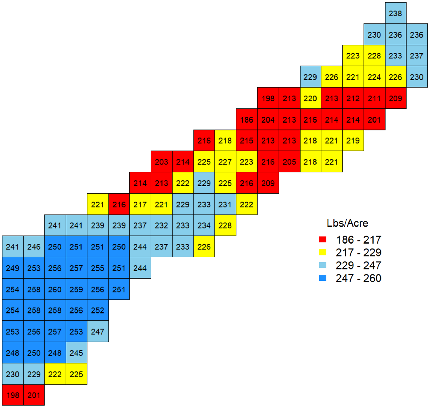
Figure 3. Estimated optimal nitrogen rate.
The spatial variation in recommended nitrogen is less than that found by Lambert and Cho (Reference Lambert and Cho2022) and by Poursina and Brorsen (Reference Poursina and Brorsen2021). These two papers had a single year of data. Also, Cho and Lambert did not use Bayesian methods, while Poursina and Brorsen used weakly informative priors and a production function that was linear in the parameters. The informative priors and multiple years of data used here led to a less noisy result.
The net return distributions under variable rates ( ${N_k^*}$
) were compared to those from uniform rate (Ñ) applications. Figure 4 plots the predictive net return distributions of the uniform and variable-rate recommendations for a location with a large difference between the two recommendations. The nitrogen recommendation with variable rates was 260 lbs/acre and 216.28 lbs/acre from the uniform rate. The variable rate encourages applying more nitrogen for locations with more production potential. As a result, variable rates generate higher net returns than uniform rates. The finding of precision application using more nitrogen is in contrast to Diacono et al. (Reference Diacono, Rubino and Montemurro2013), who concluded that precision nitrogen lowered input use, but is consistent with economic studies like Biermacher et al. (Reference Biermacher, Brorsen, Epplin, Solie and Raun2009). Since the technology increases yield, it would make a small contribution to the yield increases that will be needed due to the expected yield losses from climate change (Lee, Ji, and Moschini, Reference Lee, Ji and Moschini2022).
${N_k^*}$
) were compared to those from uniform rate (Ñ) applications. Figure 4 plots the predictive net return distributions of the uniform and variable-rate recommendations for a location with a large difference between the two recommendations. The nitrogen recommendation with variable rates was 260 lbs/acre and 216.28 lbs/acre from the uniform rate. The variable rate encourages applying more nitrogen for locations with more production potential. As a result, variable rates generate higher net returns than uniform rates. The finding of precision application using more nitrogen is in contrast to Diacono et al. (Reference Diacono, Rubino and Montemurro2013), who concluded that precision nitrogen lowered input use, but is consistent with economic studies like Biermacher et al. (Reference Biermacher, Brorsen, Epplin, Solie and Raun2009). Since the technology increases yield, it would make a small contribution to the yield increases that will be needed due to the expected yield losses from climate change (Lee, Ji, and Moschini, Reference Lee, Ji and Moschini2022).
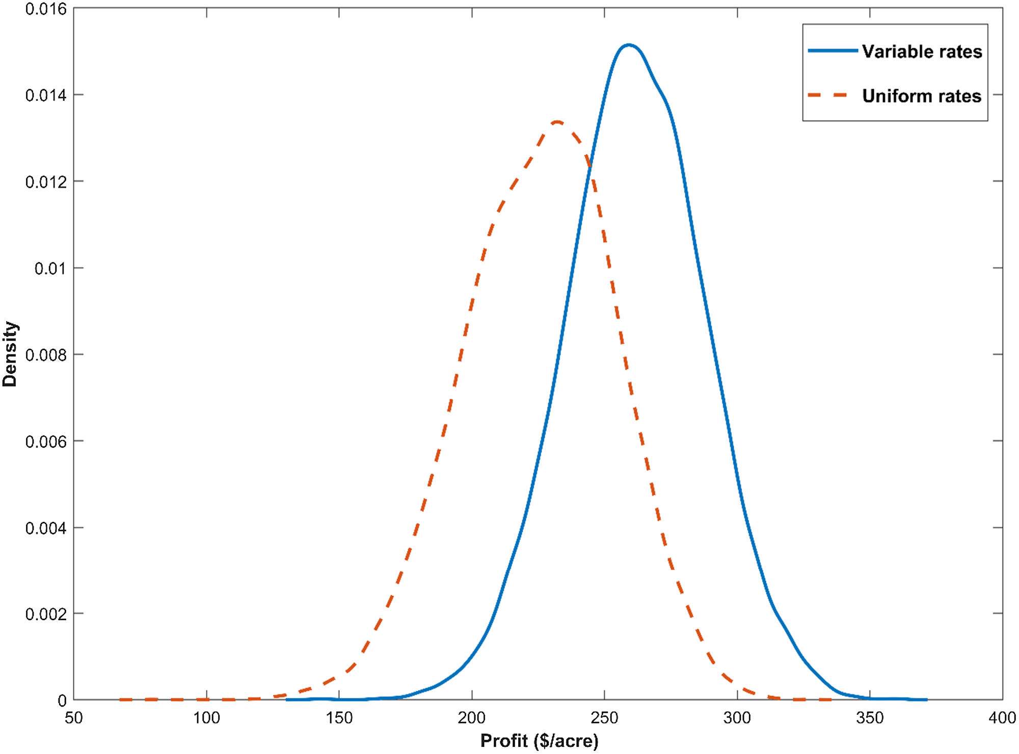
Figure 4. Posterior predictive net return densities from the uniform and variables input recommendations.
Figure 5 illustrates the mean of the net returns distribution for each location from the uniform target rates (Ñ) and the variable rates ( ${N_k^*}$
). The figure highlights how the variable rates become more profitable than the uniform rates. The predicted net returns of Ñ and
${N_k^*}$
). The figure highlights how the variable rates become more profitable than the uniform rates. The predicted net returns of Ñ and ${N_k^*}$
in the lower-plateau area (upper-right side) were almost identical. In contrast, the net returns generated from the variable rates in the higher-plateau area (lower-left side) are clearly more profitable than the uniform rates. The variable rates apply more nitrogen in areas with more production potential. The average net return of the entire field from the variable rate (
${N_k^*}$
in the lower-plateau area (upper-right side) were almost identical. In contrast, the net returns generated from the variable rates in the higher-plateau area (lower-left side) are clearly more profitable than the uniform rates. The variable rates apply more nitrogen in areas with more production potential. The average net return of the entire field from the variable rate ( ${N_k^*}$
) was $197.79/acre, and the uniform target nitrogen rate (Ñ) was $188.63/acre. The $9.16/acre economic return is favorable relative to the $1.81/acre found by Queiroz et al. (Reference Queiroz, Perrin, Fulginiti and Bullock2023) using electrical conductivity and not considering the cost of collecting the information.
${N_k^*}$
) was $197.79/acre, and the uniform target nitrogen rate (Ñ) was $188.63/acre. The $9.16/acre economic return is favorable relative to the $1.81/acre found by Queiroz et al. (Reference Queiroz, Perrin, Fulginiti and Bullock2023) using electrical conductivity and not considering the cost of collecting the information.
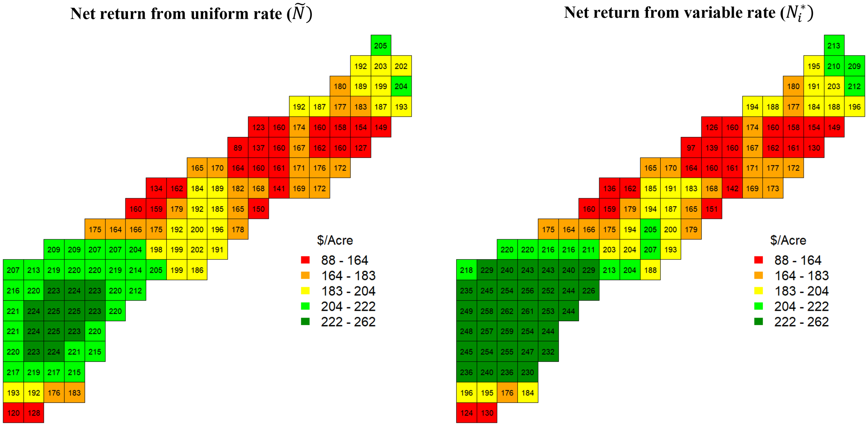
Figure 5. Posterior predictive net return for each cell.
The $9.16/acre comes from two sources: variable-rate application and more accurate modeling of the production function. How much of the $9.16/acre could be obtained by just applying a higher uniform rate? The optimal uniform rate, say Ñ $^*$
, is the rate that maximizes the entire field’s average net return via the estimated site-specific stochastic plateau model. The grid-search method was used to get Ñ
$^*$
, is the rate that maximizes the entire field’s average net return via the estimated site-specific stochastic plateau model. The grid-search method was used to get Ñ $^*$
∈ S, where S = {0, 1, …, 500}. The estimation procedure was similar to the procedure for the optimal variable rate
$^*$
∈ S, where S = {0, 1, …, 500}. The estimation procedure was similar to the procedure for the optimal variable rate ${N_k^*}$
. The estimated Ñ
${N_k^*}$
. The estimated Ñ $^*$
= 237 lbs/acre, and the entire field’s average net return was $194.10/acre. So, the variable rate
$^*$
= 237 lbs/acre, and the entire field’s average net return was $194.10/acre. So, the variable rate ${N_k^*}$
gives $3.69/acre additional net returns, and thus $5.47/acre of the benefits from using this approach could be obtained even without applying a variable rate.
${N_k^*}$
gives $3.69/acre additional net returns, and thus $5.47/acre of the benefits from using this approach could be obtained even without applying a variable rate.
Sellars et al. (Reference Sellars, Schnitkey and Gentry2020) find that producers apply more nitrogen than the maximum return to nitrogen (Sawyer et al., Reference Sawyer, Nafziger, Randall, Bundy, Rehm and Joern2006) recommended by Extension. Bullock et al. (Reference Bullock, Mieno and Hwang2020) find that the return from on-farm experiments comes from more accurate uniform rates than from site-specific technology (SST), which agrees with the findings here. So even though variable rates used more nitrogen than uniform rates, the variable rate may be less than what producers now typically apply. Therefore, the precision agriculture technology proposed here could contribute to the goal of lower applied levels of nitrogen considered by Späti et al. (Reference Späti, Huber, Logar and Finger2022). Bullock et al. (p. 1028) say that “unless more information can be produced about yield response, the profitability of SST will remain limited.” The method here can provide some of the needed information and do so at low cost.
5. Future extensions of the approach
The information provided by the method developed here is not expected to be enough by itself to justify variable-rate nitrogen application. This information is intended to complement rather than replace alternative sources of information. Since it may not be obvious to readers, we discuss how this information could be combined with other information to possibly produce profitable variable-rate nitrogen systems.
The priors used here could be improved. Soil type and elevation (Hegedus and Maxwell, Reference Hegedus and Maxwell2022) could potentially be used to specify priors that varied spatially. Future research can provide priors for the intercept and slope that are specific to the location of the field rather than using estimates from Tennessee for a field in Mississippi as was done here. We do not use the yield goal approach that has been criticized by Rodriguez et al. (Reference Rodriguez, Bullock and Boerngen2019) among others. However, the prior for the plateau was based on Mississippi Extension recommendations which do use the yield goal approach. The databases from on-farm experiments could potentially be used to estimate more precise production functions to use as priors.
The slope and intercept parameters were not included in the likelihood function due to limited data. It is possible to include them and to rely less on the priors if the level of nitrogen applied varied by year as with on-farm experiments (Hegedus and Maxwell, Reference Hegedus and Maxwell2022). The amount of nitrogen applied was expected to be greater than the agronomic optimum for most plots (Oglesby et al., Reference Oglesby, Dhillon, Fox, Singh, Ferguson, Li, Kumar, Dew and Varco2023) so the plateau would be the only parameter that could be observed for most plots.
The priors would then be used along with the methods described here to provide a posterior distribution. Going forward, nitrogen would no longer be applied at a constant rate across the field. Experimentation could be used. The vision is that the approach used here would be used prior to doing on-farm experimentation.
This posterior distribution could be used to design an optimal on-farm experiment (Poursina et al., Reference Poursina, Brorsen and Lambert2023). While they did not have spatially varying parameters, Ng’ombe and Brorsen (Reference Ng’ombe and Brorsen2022) argued for using a few small plots to reduce the cost of using nonoptimal levels of nitrogen. Li et al. (Reference Li, Mieno and Bullock2023) find that a randomized design may not be the best choice, but do not explore what levels of input to use.
After the first year of on-farm experiments, a new posterior distribution could be obtained. This distribution would then be used to select nitrogen levels in the second year.
This process would eventually converge and at some point, on-farm experimentation might no longer be needed. Due to possible structural change, however, a producer might continue doing experimentation. Corn yields have gone up over time. An increasing trend in corn yields could be modeled by letting the plateau or other parameters change with time as in Patterson (Reference Patterson2023). The trend parameters might be estimated using information from studies such as that used for maximum return to nitrogen (Nafziger et al., Reference Nafziger, Sawyer, Laboski and Franzen2022).
The beauty of the Bayesian approach is that it can readily combine information from a variety of sources. For example, the plateau could be made a function of rainfall or information from satellite imagery (Sartore et al., Reference Sartore, Rosales, Johnson and Spiegelman2022).
6. Conclusions
Previous literature evaluating variable-rate nitrogen response relied on whole-field experiment datasets with variable-rate nitrogen application. Most historical yield datasets from farmers, however, are from fields where a uniform rate was applied to the entire field. The method proposed here provides a way to use the yield information from uniform rate applications to make precision nitrogen recommendations.
A spatially varying linear response stochastic plateau model was estimated by a Bayesian Kriging approach, which allows for estimating a spatially varying plateau. The other parameters of the production function were based on prior information. The approach succeeded in providing site-specific nitrogen recommendations. The net return calculation shows that the variable rate adds approximately $9/acre. Bayesian Kriging works even when the number of observations of each cell was only five years.
Is $9/acre enough to spur adoption? The technology to apply variable-rate bulk fertilizer is already available. The yield-monitor data are already being collected so the data collection costs could be low. One drawback of the approach is that it is currently computationally expensive. While the computational burden is greatly reduced by using the HMC algorithm, it is possible to develop a commercial approach that is much faster. The key computational burden is in estimating the spatial parameters. As knowledge is gained, commercial applications may be able to assume values for these parameters or use a two-step estimator. Future research should consider basis functions (Cressie et al., Reference Cressie, Sainsbury-Dale and Zammit-Mangion2022) as a way to speed up the calculations to make the approach commercially feasible.
There are inviting ways to increase the profitability of using variable rates. One straightforward way is to use a finer grid than 100 m by 100 m. Reducing the computational burden would make this feasible. More years of data will increase the accuracy and the value of our method. The Mississippi Delta field studied is relatively uniform and less uniform fields would provide more benefit from a variable rate.
While a $9/acre in-sample return may not be enough to spur adoption, the Bayesian approach provides a ready way to combine yield-monitor data with other types of information. As others build a database from whole-field experiments, such data can be used to create informative priors based on slope, soil type, and other measures. For in-season applications, the yield-monitor data could provide priors to be combined with plant sensing data from satellites or in-field experiments such as a nitrogen-rich strip. Whole-field predictions based on weather data can be readily combined with yield-monitor data using Bayesian methods. Combining with these other sources of information provides an opportunity to overcome the economic hurdle and deliver the promises of digital agriculture to nitrogen application. One major point is that we need to be saving yield-monitor data even when a uniform rate was applied because such data can be useful in making precision nitrogen recommendations.


 Open access