


1. Introduction
Micro-air vehicles (MAVs) are of great value in both military and civilian applications, powering the advance of studies in low-Reynolds-number aerodynamics  $\textit {O}(10^2\unicode{x2013}10^5)$. Previous researches have established that the thin flat plate provides a higher lift-to-drag ratio at low Reynolds numbers, compared with the conventional thick aerofoil (McMasters & Henderson Reference McMasters and Henderson1980; Mueller Reference Mueller1999). The effects of aspect ratio ( $A\!R$) and planform shape on aerodynamic characteristics have been considered (Torres & Mueller Reference Torres and Mueller2001; Okamoto & Azuma Reference Okamoto and Azuma2011; Ananda, Sukumar & Selig Reference Ananda, Sukumar and Selig2015; Mizoguchi, Kajikawa & Itoh Reference Mizoguchi, Kajikawa and Itoh2016; Okamoto et al. Reference Okamoto, Sasaki, Kamikubo and Fujii2019). It has been shown that wings with $A\!R\gtrsim 1$ exhibit the maximum lift-to-drag ratio within the angle of attack range $\alpha \approx 4^\circ \unicode{x2013}10^\circ$, regardless of the various planform shapes tested. The occurrence of the laminar separation bubble (LSB) within this $\alpha$ range has also been verified via flow visualizations in these studies.
To gain insight into how the tip effects impact the unsteady behaviour of the LSB over wings, extensive attention has been paid to the three-dimensional (3-D) flow structures (Burgmann, Brücker & Schröder Reference Burgmann, Brücker and Schröder2006; Burgmann, Dannemann & Schröder Reference Burgmann, Dannemann and Schröder2008; Burgmann & Schröder Reference Burgmann and Schröder2008; Hain, Kähler & Radespiel Reference Hain, Kähler and Radespiel2009; Kurelek, Lambert & Yarusevych Reference Kurelek, Lambert and Yarusevych2016; Zhang et al. Reference Zhang, Hayostek, Amitay, He, Theofilis and Taira2020; Toppings, Kurelek & Yarusevych Reference Toppings, Kurelek and Yarusevych2021; Toppings & Yarusevych Reference Toppings and Yarusevych2021). Burgmann et al. (Reference Burgmann, Dannemann and Schröder2008) investigated experimentally the unsteady vortical structures over an SD7003 aerofoil at  $\alpha = 4^\circ \unicode{x2013}8^\circ$ for the chord-based Reynolds numbers of $Re_c = (2\unicode{x2013}6)\times 10^4$. They found that the shed vortices exhibited C-shape structures. As evolving downstream, the C-shape vortices transformed into the screwdriver vortices. This transformation arises from the entrainment of freestream fluid on the leeward sides of the C-shape vortices, which forces the vortex heads to slow down and contract. To demonstrate the tip effects on the structure and dynamics of the LSB, Toppings & Yarusevych (Reference Toppings and Yarusevych2021) measured the flow over a finite- $A\!R$ (semi- $A\!R=2.5$) NACA0018 wing. It was shown that the flow was governed largely by the tip effects in the near-tip region, while remaining relatively two-dimensional (2-D) in the inboard region. Despite the spanwise variation in the flow, the fundamental vortex shedding characteristics remained largely invariant. Moreover, the flow structures over finite- $A\!R$ wings at $Re_c=400$ were studied numerically by Zhang et al. (Reference Zhang, Hayostek, Amitay, He, Theofilis and Taira2020). Near the wingtip, the shed vortices featured 3-D braid-like structures. These braid-like structures connected the spanwise coherent leading-edge vortices (LEVs) and trailing-edge vortices (TEVs) to form closed vortex loops in the wake.
Regarding low- $A\!R$ plates ( $A\!R\lesssim 2$), the flows become highly 3-D under the stronger tip effects. DeVoria & Mohseni (Reference DeVoria and Mohseni2017) reported experimentally that the downwash of the tip vortices (TiVs) facilitates the flow reattachment when $A\!R$ is sufficiently small ( $A\!R<1.5$). It can be inferred from the numerical simulations that due to the downwash, the periodically shed vortices (e.g. LEVs) exhibited hairpin structures at $Re_c=300\unicode{x2013}500$ (Taira & Colonius Reference Taira and Colonius2009b; Tong, Yang & Wang Reference Tong, Yang and Wang2020). Apart from the downwash flow, there is a strong spanwise flow near the plate surface, arising from the spanwise pressure gradient induced by the tip effects (Visbal Reference Visbal2011, Reference Visbal2012; Visbal & Garmann Reference Visbal and Garmann2012). The spanwise flow, directed from the plate tips towards the midspan, brings about the formation of two unstable foci in the limiting streamline pattern. A similar topological pattern has been observed in experimental studies, with oil flow visualizations (Chen, Bai & Wang Reference Chen, Bai and Wang2016) and particle image velocimetry (PIV) measurements (Gresham, Wang & Gursul Reference Gresham, Wang and Gursul2010). These studies show that the near-wall spanwise flow is prevalent for the flows over low- $A\!R$ wings.
So far, the influence and the underlying mechanisms of the near-wall spanwise flow are not fully understood, limiting the development of high-performance MAVs.A comprehensive description of the vortex evolution is essential to address these issues. However, few relevant experimental studies can be found in the literature, which is due mainly to several limitations (e.g. low spatial resolution, high cost) of the existing 3-D and three-component (3-D3-C) flow-field diagnostic techniques, such as scanning stereoscopic PIV and tomographic PIV. In this paper, a 3-D3-C flow-field reconstruction method is proposed to synchronize multi-plane PIV data and provide new insights into complex 3-D flows. On this basis, the 3-D flow evolution over a low- $A\!R$ trapezoidal plate is characterized. The focus is laid on the near-wall spanwise flow. Its interactions with the vortical structures are essential for improving the flight performance of MAVs. Thus this study will help to deepen understanding of the interaction mechanism of coherent structures in low-Reynolds-number flows.
The remainder of this paper is organized as follows. In § 2, the experimental set-up and the post-processing tools are described, including the proposed 3-D3-C flow-field reconstruction method. Subsequently, the development of the separation bubble with the angle of attack is presented in § 3, and a novel bubble structure is displayed. This bubble structure is explored further with respect to its spatial characteristics in § 4, and the corresponding vortex dynamics in § 5. Specifically, the interactions of the vortices with the near-wall spanwise flow are revealed in § 5.3. The interaction mechanism and its significance on the flight performance of MAVs are discussed in § 6. Finally, conclusions are drawn in § 7.
2. Experimental methodology
2.1. Experimental set-up
The experiments are conducted at the low-speed recirculation water channel in Beijing University of Aeronautics and Astronautics, China. The test section is  $600\ {\rm mm}\times 600 \ {\rm mm}\times 3000\ {\rm mm}$ (height $\times$ width $\times$ length). The separated flow over a low- $A\!R$ trapezoidal plate is investigated, as shown in figure 1. The rigid flat plate is constructed from a $1$ mm thick aluminium sheet; all edges are left square. The planform shape is depicted in figure 1(a). In the natural world, similar trapezoidal planform shapes are utilized by numerous animals when gliding, including the flying squirrel and the flying lemur bat. The study of the trapezoidal plate has value in advancing our understanding of the remarkable gliding capacities of these animals. Furthermore, the vortex dynamics for the trapezoidal plate are influenced significantly by the tip effects, as demonstrated via flow visualization in Appendix A. Recalling the motivation of this study, which is to explore in depth the tip effects for low- $A\!R$ plates, the flow over the trapezoidal plate is a valuable subject to investigate. The chord length of the plate is $c=58$ mm, giving thickness-to-chord ratio $1.7\,\%$. The leading- and trailing-edge lengths are $L_l=80$ mm and $L_t=58$ mm (equal to the chord length), respectively. The taper angle of the side edges is $\beta =12^\circ$. In this paper, $A\!R$ is defined as the ratio of maximum span to chord, $A\!R\equiv L_{max}/c = L_l/c=1.38$. The freestream velocity is set at $U_\infty =96$ mm s $^{-1}$, and the chord-based Reynolds number is approximately $Re_c=5800$. This value falls within the operating range for flying insects ( $Re_c=10^3\unicode{x2013}10^4$).

Figure 1. (a) Planform shape and dimensions of the plate. The dashed circle depicts the position where the plate is glued on the round rod. (b) Experimental set-up for the 3-C PIV configuration. (c) Plate support system.
As shown in figure 1(b), the plate is hung upside down into the water channel test section with a square strut connected to a translator. The orientation of the translator can be modified to shift the plate in either the freestream or the spanwise direction with resolution 0.1 mm. The plate is covered with matt black paint to attenuate the undesired light reflections. The detailed plate support system is sketched in figure 1(c). The plate is glued on a round rod (4 mm diameter, 100 mm length) with acrylate adhesive. The round rod is connected to the square strut with a square rod. Meanwhile, a mechanical inclinometer is designed to manually adjust the angle between the strut and the rods with resolution  $0.5^\circ$. The support system is firmly attached with two bolts B1. By adjusting the orientation of the rods, four angles of attack are tested in this study, namely $\alpha =4^\circ$, $6^\circ$, $8^\circ$ and 10 $^\circ$. After each angle adjustment, a bolt B2 is used to lock the rods.
Two coordinate systems are used for data presentation, as shown in figure 2. One is the natural coordinate system  $O$-
$O$- $xyz$, where the origin $O$ is defined so that the point at the trailing edge at the midspan is $(c,0,0)$ (as illustrated with the red point in figure 2b), and the three axes $(x,y,z)$ are along the streamwise, vertical and spanwise directions, respectively. The other is the plate-based coordinate system $\hat {O}$- $\hat {x}\hat {y}\hat {z}$, where the origin $\hat {O}$ is set at the leading edge at the midspan, and the three axes $(\hat {x},\hat {y},\hat {z})$ are along the chordwise, wall-normal and spanwise directions, respectively. Since the $z$-axis and the $\hat {z}$-axis have the same direction and scale, only the $z$-axis is retained to describe the spanwise position, for simplicity.

Figure 2. Sketch of the coordinate systems and the PIV measurement planes: (a) plan view; (b) side view (midspan plane).
2.1.1. Particle image velocimetry
Two PIV configurations are set up to conduct the quantitative flow-field measurements, i.e. the three-component (3-C) and two-component (2-C) PIV configurations. The detailed parameters for both PIV configurations are listed in table 1.
Table 1. PIV measurement parameters.

For the 3-C PIV configuration, the stereoscopic PIV technique is adopted to obtain the statistical characteristics of the flow fields. As sketched in figure 1(b), the water channel is seeded with hollow glass beads of 5–20  $\mathrm {\mu }$m diameter and illuminated with a dual-head Nd:YAG laser (Beamtech Vlite-500). The thickness of the light sheet is 2 mm. Two charged-coupled device (CCD) cameras (IMPERX ICL-B2520M, $2456\times 2058$ pixels) are arranged on each side of the water channel. These cameras are equipped with Nikkor 85 mm tilt-shift lenses and satisfy the Scheimpflug condition. The viewing angles of these cameras are approximately ${\pm }65^\circ$ (Nobes, Wieneke & Tatam Reference Nobes, Wieneke and Tatam2004). The cameras and the laser are synchronized using a MicroVec Micropulse-725 synchronizer. Particle images are acquired in a double-frame mode at frequency 3 Hz. In this configuration, 3-C velocity fields in $21$ closely spaced $y$–
$y$– $z$ planes are measured by shifting the plate in the streamwise direction through the stationary light sheet. The measurement planes range from $x/c=-0.03$ to $x/c=1.00$ with increment $\Delta x/c\approx 0.052\ (3\ {\rm mm})$, as illustrated with the red lines in figure 2(a). For each plane, a total of $2000$ image pairs are obtained.
For the 2-C PIV configuration, the time-resolved PIV measurements are performed with a focus on the dynamics of the LEVs. The flow is illuminated by the  $1$ mm thick light sheet, which is generated by a semiconductor continuous laser (8 W, 532 nm). Particle images are recorded using a high-speed CMOS camera (Photron Fastcam SA2 86K-M3) at sampling rate 288 Hz. The images are cropped to $832 \times 2048$ pixels, and the field of view is approximately $0.52c\times 1.31c$. Considering the symmetry of the flow fields, 2-C velocity fields in four $x$–
$x$– $y$ planes, $z/c=0,0.05,0.12,0.24$ (blue lines in figure 2a), are measured by shifting the plate along the $z$-axis. For each plane, a repetition of $13\,432$ images is obtained, continuously spanning approximately $240$ LEV shedding cycles.
All particle images are pre-processed using the POD-based background removal method (Mendez et al. Reference Mendez, Raiola, Masullo, Discetti, Ianiro, Theunissen and Buchlin2017), and the 2-D2-C velocity vectors are calculated using the multi-pass iterative Lucas–Kanade (MILK) algorithm (Champagnat et al. Reference Champagnat, Plyer, Le Besnerais, Leclaire, Davoust and Le Sant2011; Pan et al. Reference Pan, Xue, Xu, Wang and Wei2015) with four pyramid levels and three Gauss–Newton iterations per level. The interrogation window sizes are set to  $48 \times 48$ and $32 \times 32$ pixels for the 3-C and 2-C PIV configurations, respectively. Regarding the stereoscopic PIV scenario, the stereoscopic reconstruction is then performed to obtain the 2-D3-C velocity vectors using the Soloff method (Soloff, Adrian & Liu Reference Soloff, Adrian and Liu1997). Additionally, the misalignment of the calibration target with the light sheet is corrected using the self-calibration method (Wieneke Reference Wieneke2005). For both configurations, the velocity data have a similar vector pitch of approximately 0.3 mm. The raw velocity data are validated using the robust principal component analysis method (Scherl et al. Reference Scherl, Strom, Shang, Williams, Polagye and Brunton2020). The uncertainty relative to the freestream velocity is approximately $1.5\,\%$ and $1.0\,\%$ for the 3-C and 2-C velocity fields, respectively (van Doorne & Westerweel Reference van Doorne and Westerweel2007). The spanwise vorticity $\omega _z$ is computed from the 2-C PIV data using the central-difference scheme. Therefore, the vorticity calculation is not affected by the coarse streamwise resolution for the 3-C PIV configuration. Following the strategies of Qu et al. (Reference Qu, Wang, Feng and He2019), the normalized uncertainty is estimated to be $\varepsilon (\omega _z)c/U_\infty =1.35$, which is acceptable to resolve the focused flow structures.
2.1.2. Hydrogen bubble visualization
Hydrogen bubble visualization is utilized to capture the unsteady vortical structures qualitatively. A platinum wire (20  $\mathrm {\mu }$m diameter) is placed along the $z$-axis to generate a continuous sheet of hydrogen bubbles. The hydrogen bubble sheet is illuminated with white light emitting diodes. The CCD camera is positioned above the suction side of the plate, and records at sampling rate 10 Hz.
2.2. Post-processing tools
2.2.1. Proper orthogonal decomposition
Proper orthogonal decomposition (POD) is a powerful tool for detecting the large-scale coherent structures embedded in the flow. Using POD, the fluctuating part of given velocity fields can be projected on a set of orthogonal bases  $\{\varPhi _k\}$, which is optimal in an energetic sense (van Oudheusden et al. Reference van Oudheusden, Scarano, van Hinsberg and Watt2005):
 \begin{equation} \boldsymbol{u}( \boldsymbol{x},t )=\bar{\boldsymbol{u}}( \boldsymbol{x} )+\boldsymbol{u}^{\prime}( \boldsymbol{x},t ) =\bar{\boldsymbol{u}}( \boldsymbol{x} )+\sum_{k}{{{a}_{k}}(t)\,{{\varPhi}_{k}}( \boldsymbol{x} )}, \end{equation}
where  $\bar {\boldsymbol {u}}( \boldsymbol {x} )$ and $\boldsymbol {u}^{\prime }( \boldsymbol {x},t )$ represent the mean and the fluctuating components of the velocity fields, respectively. Also, ${{a}_{k}}(t)$ denotes the mode coefficient at a snapshot instant $t$ corresponding to the $k$th POD mode $\varPhi _k$. The POD modes are obtained by solving the eigenvalue problem of the time-averaged two-point spatial correlation matrix $\boldsymbol {C}$:
 \begin{equation} \boldsymbol{C}{{\varPhi }_{k}}={{\lambda }_{k}}{{\varPhi }_{k}}, \quad \text{with}\ {{C}_{m,n}}=\overline{\boldsymbol{u}^{\prime}( {{x}_{m}},t )\,\boldsymbol{u}^{\prime}( {{x}_{n}},t )}. \end{equation}
The eigenvalue  ${\lambda }_{k}$ measures the energy contained in the $k$th POD mode. When the POD modes are ranked in descending order of the eigenvalues, the first few orthogonal modes usually contain the most energy. Thus these low-rank POD modes provide an efficient way to build a reduced-order model (ROM) for the flow fields.
Another great virtue of POD is its capability to identify the phase information for quasi-periodic flows. When flows are dominated by periodical travelling coherent structures, the corresponding phase angle  $\theta ( t )$ can be obtained with the aid of the first mode pair (Legrand, Nogueira & Lecuona Reference Legrand, Nogueira and Lecuona2011a; Toppings & Yarusevych Reference Toppings and Yarusevych2021):
 \begin{equation} \theta ( t )=\tan^{{-}1}\left( \frac{{{a}_{1}}( t )}{{{a}_{2}}( t )}\, \frac{\sqrt{2{{\lambda }_{2}}}}{\sqrt{2{{\lambda }_{1}}}} \right). \end{equation}
According to Lengani et al. (Reference Lengani, Simoni, Ubaldi and Zunino2014), the wall-normal velocity component  $\hat {v}$ is closely related to the vortex shedding phenomenon. To identify the phase information of the shed LEVs, POD is performed on this velocity component for the 2-C PIV data.
Once the phase information is determined, the instantaneous velocity vectors  $\boldsymbol {u}=(u,v)$ can be sorted along the phase angle $\theta$ and averaged using the curve-fitting method (Lengani et al. Reference Lengani, Simoni, Ubaldi and Zunino2014; Toppings & Yarusevych Reference Toppings and Yarusevych2021). Specifically, this involves applying an $8$-term Fourier model fit for the phase-sorted velocity vector at every spatial point, as illustrated in figure 3.

Figure 3. Phase averaging using Fourier series model fitting. The velocity vectors  $\boldsymbol {u}=(u,v)$ at the spatial point $(x/c,y/c,z/c)=(0.36,0.15,0)$ are extracted from the 2-C PIV data at $\alpha =6^\circ$. Contours show the distributions of the velocity components.
2.2.2. 3-D3-C flow-field reconstruction and linear stochastic estimation
To characterize the dynamical evolution of the flow structures, a 3-D3-C flow-field reconstruction method is proposed. This method links the velocity data from the 3-C and 2-C PIV measurements to restore the phase-averaged 3-D coherent structures.
The spatial consistency between the PIV measurement planes is the key to the proposed reconstruction method. The spatial distribution of the planes is sketched in figure 4(a). The reconstruction domain is indicated by the dashed box. Due to the light sheet reflections, flow fields under height  $\hat {y}/c=0.016\ (0.9\ {\rm mm})$ are excluded from the reconstruction. The 2-C velocity fields in the plane $z/c=0$ (blue) are denoted as ${\boldsymbol {u}_{2\text {-}C}}( \boldsymbol {x}_{( 0 )},t )$; the 3-C velocity fields in the given plane $x/c=x^\ast$ (one of the red planes) are denoted as ${{\boldsymbol {u}}_{3\text {-}C}}( {{\boldsymbol {x}}_{( \ast )}},\tau )$. The planes $\boldsymbol {x}_{( 0 )}$ and $\boldsymbol {x}_{( \ast )}$ intersect in the line (the matched one of the yellow lines) denoted as $\boldsymbol {x}_{line}$. Notably, these intersection lines provide an opportunity to restore the global flow information from the asynchronously measured local velocity fields. Specifically, the linear stochastic estimation (LSE) method (Adrian Reference Adrian1994; Podvin et al. Reference Podvin, Nguimatsia, Foucaut, Cuvier and Fraigneau2018) is adopted to link the asynchronous data in every two orthogonal planes, inspired by the work of Dellacasagrande et al. (Reference Dellacasagrande, Verdoya, Barsi, Lengani and Simoni2021).

Figure 4. (a) Schematic of the PIV measurement planes used for reconstruction. (b) Flowchart of the reconstruction method.
The proposed reconstruction method contains three main steps, as illustrated in figure 4(b). The first step is to establish a ROM for the 3-C velocity fields  ${{\boldsymbol {u}}_{3\text {-}C}}( {{\boldsymbol {x}}_{( \ast )}},\tau )$ using POD:
 \begin{equation} {{\boldsymbol{u}}_{3\text{-}C}}( {{\boldsymbol{x}}_{({\ast} )}},\tau ) ={{\bar{\boldsymbol{u}}}_{{3\text{-}C}({\ast} )}}+{\boldsymbol{u}^{\prime}_{3\text{-}C}}( {{\boldsymbol{x}}_{({\ast} )}},\tau ) ={{\bar{\boldsymbol{u}}}_{{3\text{-}C}({\ast} )}}+\sum_{k=1}^{R}{{{a}_{k}}( \tau )\,{{\varPhi }_{k}}}. \end{equation}
Here, the truncation rank (TR)  $R$ is determined using the cumulative energy criteria with cutoff threshold $90\,\%$.
Next, the LSE method is utilized to conveniently calibrate the linear mapping factor  $\boldsymbol {M}_k$ between the $k$th POD mode coefficients ${a}_{k}( \tau )$ and the fluctuating velocity fields ${\boldsymbol {u}^{\prime }_{2\text {-}C}}( \boldsymbol {x}_{line},\tau )$:
 \begin{equation} \overline{{\boldsymbol{u}^{\prime}_{2\text{-}C}}( m,\tau )\,{\boldsymbol{u}^{\prime}_{2\text{-}C}}( n,\tau )}\,{{M}_{km}} =\overline{{{a}_{k}}( \tau )\,{\boldsymbol{u}^{\prime}_{2\text{-}C}}( n,\tau )}, \quad \text{with}\ m,n\in {{\boldsymbol{x}}_{{line}}}. \end{equation}
Here, the  ${\boldsymbol {u}^{\prime }_{2\text {-}C}}( \boldsymbol {x}_{line},\tau )$ are composed of the $(u,v)$ components and collected from the 3-C velocity fields ${\boldsymbol {u}_{3\text {-}C}}( \boldsymbol {x}_{(\ast )},\tau )$. Once the factor $\boldsymbol {M}_k$ is calibrated, the pseudo-mode coefficient at a given reference instant $t_{ref}$ can be estimated as
 \begin{align} {{a}_{k,est.}}( {{t}_{{ref}}} ) =\text{linear estimate of }\mathbb{E}\{ {{a}_{k}}( {{t}_{{ref}}} )\mid {\boldsymbol{u}^{\prime}_{2\text{-}C}}( {{\boldsymbol{x}}_{{line}}},{{t}_{{ref}}} )\} ={{\boldsymbol{M}}_{k}}\,{\boldsymbol{u}^{\prime}_{2\text{-}C}}( {{\boldsymbol{x}}_{{line}}},{{t}_{{ref}}} ), \end{align}
where  $\mathbb {E}\{ {\cdot } \}$ is the expectation operator, and ${\boldsymbol {u}^{\prime }_{2\text {-}C}}( {{\boldsymbol {x}}_{{line}}},{{t}_{{ref}}} )$ are the reference signals for estimation. Intuitively, the reference signal can be extracted from the original 2-C velocity fields ${\boldsymbol {u}_{2\text {-}C}}( \boldsymbol {x}_{( 0 )},t )$.
Finally, to take advantage of the linearity of the mapping matrix  $\boldsymbol {M}_k$, the pseudo-mode coefficients are estimated using the phase-averaged velocity fields ${\boldsymbol {u}_{2\text {-}C}}( \boldsymbol {x}_{( 0 )},\theta )$ rather than the original ones ${\boldsymbol {u}_{2\text {-}C}}( \boldsymbol {x}_{( 0 )},t )$. This modification filters out the secondary cycle-to-cycle variations to reveal the primary evolution of LEVs, as demonstrated in § 5.1. Note that the pseudo-mode coefficients for different planes $\boldsymbol {x}_{( \ast )}$ are synchronized with the reference phase angle $\theta$. Thus the phased-averaging 3-D3-C flow fields are reconstructed as follows:
 \begin{equation} {\boldsymbol{u}}_{{est.}}( {{\boldsymbol{x}}_{({\ast} )}},\theta ) ={{\bar{\boldsymbol{u}}}_{{3\text{-}C}({\ast} )}}+\sum_{k=1}^{R}{{{\boldsymbol{M}}_{k({\ast} )}}\,{\boldsymbol{u}^{\prime}_{2\text{-}C}}( {{\boldsymbol{x}}_{{line}}},\theta )\,{{\varPhi }_{k}}} \quad \text{for}\ 0.17 \leq {{x}^{{\ast}}} \leq 0.95. \end{equation}
3. Separation bubble development
The separation bubble emerges at  $\alpha =6^\circ$ and changes its structure with increasing
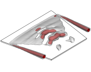
  $\alpha$. Figure 5 presents the time-averaged spatial structures, which are constructed from the measured 3-C PIV data. The 3-D shapes of the separation bubbles are illustrated with the iso-surfaces of $\bar {u}/U_\infty =0$ in transparent grey. To better visualize the internal structures of the separation bubbles, two iso-surfaces of $\bar {u}/U_\infty =-0.15$ (transparent blue) and $\bar {u}/U_\infty =-0.2$ (red) are presented inside the transparent grey iso-surfaces. In figure 5(a), the grey iso-surface concaves downwards near the midspan with increasing $x/c$, and the blue iso-surface bifurcates around $x/c=0.48$. These observations reveal that the separation bubble features a distinct structure resembling the tail of a swallow at $\alpha =6^\circ$. This swallow-tailed structure can also be observed at $\alpha =8^\circ$ (figure 5b). It is noticed that the separation bubble increases in wall-normal extent faster near the midspan than in the lateral portions with increasing $\alpha$. Consequently, at $\alpha =10^\circ$ (figure 5c), the separation bubble exhibits a single-tailed structure, which is well-known for flow over low- $A\!R$ plates (Chen et al. Reference Chen, Bai and Wang2016). Meanwhile, the spatial distribution of the blue and red iso-surfaces is quite different from that at the smaller $\alpha$.

Figure 5. Oblique view of the time-averaged separation bubbles. The transparent grey iso-surfaces correspond to  $\bar {u}/U_\infty =0$ and represent the 3-D shapes of the separation bubbles. Inside the transparent grey iso-surfaces, the transparent blue and red iso-surfaces correspond to $\bar {u}/U_\infty =-0.15$ and $-0.2$, respectively. They depict the internal structures of the separation bubbles.
To better understand the structural change of the separation bubble, figure 6 presents the near-wall representations of the flows at  $\hat {y}/c=0.026$, which are also constructed from the measured 3-C PIV data. Once the flow separates, two unstable foci N1, N2, and a saddle point S1 (illustrated with black dots), form. The pattern of these critical points approximates the common limiting streamline topology for low- $A\!R$ plates; see e.g. Visbal (Reference Visbal2011). Furthermore, it is noted that an unstable node N3 and two saddle points S2, S3 (orange dots) form at $\alpha =6^\circ,8^\circ$, while only one saddle point S2 (red dot) forms at $\alpha =10^\circ$. This topological change verifies that the swallow-tailed structure is a novel structure that emerges at the relatively small $\alpha$.

Figure 6. Time-averaged streamline patterns in the plane  $\hat {y}/c=0.026$. The critical points are marked with dots.
The formation of the swallow-tailed separation bubble seems counterintuitive given the conventional understanding of the tip effects. Since the downwash weakens as the distance to the TiVs increases according to the Biot–Savart law, the downwash has a minimal influence on the swallow-tailed separation bubble (as demonstrated in Appendix B). Therefore, there must be an additional source responsible for the formation of the swallow-tailed structure. In the rest of this paper, attention is concentrated on the swallow-tailed separation bubble at  $\alpha =6^\circ$. The near-wall spanwise flow, also induced by the tip effects, is explored to account for the formation of the swallow-tailed structure.
4. Characteristics of the swallow-tailed separation bubble
In this section, the velocity distributions inside the swallow-tailed separation bubble are investigated in detail to highlight the structural characteristics. Figure 7(a) presents the time-averaged spanwise velocity field in the plane  $\hat {y}/c=0.026$. Evident spanwise flow occurs above the plate surface, directed towards the midspan (indicated by black arrows). The near-wall spanwise flow region is demarcated by the magenta solid lines ( $\bar {w}/U_\infty =\pm 0.1$). To quantify the spatial distribution of the near-wall spanwise flow, the spanwise interval of the near-wall spanwise flow region, $d_w(x,\theta )$, is hereinafter defined as the spanwise extent of the region where $| w/U_\infty | \leq 0.1$ near the midspan at $\hat {y}/c=0.026$. Most notably, the time-averaged spanwise interval $\bar {d}_w$ remains next to its minimum value in the streamwise range $x/c\in [ 0.38,0.59 ]$, which is masked in grey in figure 7(a). To locate the separation bubble, its sectional shape and the internal structure are presented using the blue solid and dashed lines of $\bar {u}/U_\infty =0$ and $-0.15$, respectively. Interestingly, this streamwise range $x/c\in [ 0.38,0.59 ]$ is where the $\bar {u}/U_\infty \leq -0.15$ region (demarcated by the blue dashed line) bifurcates. This suggests that the near-wall spanwise flow plays a crucial role in the formation of the swallow-tailed separation bubble.

Figure 7. (a) Time-averaged spanwise velocity field in the plane  $\hat {y}/c=0.026$. The black arrows indicate the local flow directions. The grey mask region highlights the streamwise range $x/c\in [0.38,0.59]$ where $\bar {d}_w$ is relatively small. (b) Time-averaged normal velocity field in the plane $x/c=0.48$. In both (a,b), the blue solid and dashed lines are the contour lines of $\bar {u}/U_\infty =0$ and $-0.15$, respectively. The magenta solid lines are the contour lines of $\bar {w}/U_\infty =\pm 0.1$.
To gain more vivid insights into the influence of the near-wall spanwise flow on the separation bubble structure, figure 7(b) presents the time-averaged vertical velocity field near the separation bubble in the plane  $x/c=0.48$. Considering the symmetry of the time-averaged flow, only the flow field in the positive portion ( $z \geq 0$) of the plate is shown. A local upwash region (indicated by arrow $A$) occurs near the $\bar {u}/U_\infty \leq -0.15$ region (demarcated by the blue dashed line, arrow $B$). Meanwhile, the near-wall spanwise flow region (demarcated by the magenta solid line) is elongated in the spanwise direction and overlaps the centres of regions $A$ and $B$. This phenomenon can be explained as follows. From the perspective of mass conservation of a fluid element in the near-wall spanwise flow region, the spanwise flow drives the mass transport from the plate tips to the midspan. Additionally, the relatively small $\bar {d}_w$ gives rise to the potential mass accumulation near the midspan, which is compensated for by the strengthening of the upwash and the reverse flows. In fact, a similar upwash distribution can be seen in the streamwise range $x/c\in [ 0.38,0.59 ]$ (the grey mask region in figure 7a), where the upwash is gradually suppressed by the increase in $\bar {d}_w$ (not shown in this paper for brevity). Therefore, the near-wall spanwise flow affects the velocity distributions near the midspan, leading to the formation of the swallow-tailed separation bubble.
5. Vortex shedding within the swallow-tailed separation bubble
As demonstrated in § 4, the near-wall spanwise flow brings about noticeable local velocity modifications in the time-averaged flow field. To further determine the effects of the near-wall spanwise flow from a dynamic perspective, the vortex shedding within the swallow-tailed separation bubble is investigated in this section.
Figure 8(a) presents the hydrogen bubble visualization of the shed vortices. The platinum wire (indicated by the blue line) is arranged inside the separated shear layer at  $(x/c,y/c)=(0.11,0.13)$. The LEVs successively exhibit three kinds of structures with downstream position: (i) at $x/c\approx 0.3$, the newly born LEV1 (indicated by the red solid line) has a small spanwise extent; (ii) at $x/c\approx 0.5$, LEV2 (yellow dashed line) resembles a C-shape structure; and (iii) at $x/c\approx 0.8$, LEV3 (green dash-dotted box) appears as an M-shape structure with its core bending downstream near the midspan. It appears that the shed LEVs undergo complex transformations as they evolve downstream.

Figure 8. (a) Plan-view hydrogen bubble visualization of vortical structures over the trapezoidal plate at  $\alpha =6^\circ$. Vortices are identified by the high-concentration regions of hydrogen bubbles (blue colour). (b) Oblique view of the representative phase-averaged field (at $\theta =0^\circ$). The grey and red iso-surfaces correspond to $Qc^2/U_\infty ^2=5$ and $30$, respectively.
To characterize the LEVs quantitatively, the phase-averaged 3-D3-C flow fields are reconstructed. The validity of the reconstructed flow fields is demonstrated in Appendix C. The flow field at  $\theta =0^\circ$ is presented in figure 8(b). Vortical structures are depicted through the $Q$-criterion (Hunt, Wray & Moin Reference Hunt, Wray and Moin1988), where $Q$ is defined by the second invariant of the velocity gradient tensor, with a positive value indicating that the strength of rotation overcomes the strain in incompressible flows. The independence of the present study on the contour level of $Q$ is shown in Appendix D. In figure 8(b), the vortex cores are highlighted by the iso-surface of $Qc^2/U_\infty ^2=30$ in red. The phase-averaged flow field presents the dominant vortical structures over the trapezoidal plate, such as the LEVs and the TiVs.In particular, the LEVs exhibit successively three kinds of structures along the streamwise direction, which is consistent with the results from the hydrogen bubble visualization (figure 8a). The consistency between the qualitative visualization and the quantitative reconstruction indicates that the proposed reconstruction method can properly reflect the evolution characteristics of the LEVs. According to the morphological characteristics, these three typical structures are named in sequence as the spanwise vortex, C-shape vortex and M-shape vortex, as illustrated in figure 8(b). Moreover, the shoulders of the M-shape vortex (indicated by arrow $A$) lie above the trailing parts of the separation bubble (see the grey iso-surface in figure 5a), which suggests that the swallow-tailed structure is associated with the M-shape vortices.
5.1. Primary evolution path of leading-edge vortices
To track quantitatively the evolution of the LEVs, the positions of the vortex heads are determined first. In practice, the central positions  $(x_c,y_c)$ of the LEV heads are extracted from the phase-averaged 2-C velocity fields at $z/c=0$, ${\boldsymbol {u}_{2\text {-}C}}( \boldsymbol {x}_{( 0 )},\theta )$, which are exactly the reference signals for reconstruction. Specifically, the central positions are calculated by $x_c={\iint _{C}{x{\omega _z}\,{\rm d}s}}/{\iint _{C}{c{{\omega }_{z}}\,{\rm d}s}}$, $y_c={\iint _{C}{y{{\omega }_{z}}\,{\rm d}s}}/{\iint _{C}{c{{\omega }_{z}}\,{\rm d}s}}$, where $C$ is the integral region. Here, the integral region is defined as where $Q_{2\text {-}C}\,c^2/U_\infty ^2\geq 30$ (with $Q_{2\text {-}C}$ computed using the in-plane velocity components). The spanwise vorticity field at $\theta =0^\circ$ is shown, for example, in figure 9. The LEV heads and their central positions are illustrated with the yellow lines and crosses. The benefit of this vorticity integral method is that the LEVs can be located despite the vortex transformations along the streamwise direction.

Figure 9. Spanwise vorticity field in the plane  $z/c=0$ at $\theta =0^\circ$. The LEV heads are presented by the contour lines of $Q_{2\text {-}C}\,c^2/U_\infty ^2=30$ in yellow, with the central positions marked by the yellow crosses.
Figure 10 illustrates the LEV evolution as a function of the extended phase angle  $\theta _c$ (or the streamwise position of the LEV head $x_c$). For $\theta _c\leq 240^\circ$ (or $x_c\leq 0.4$), the spanwise extent of the spanwise vortex increases with $\theta _c$. Meanwhile, the newly formed lateral arms are located further downstream relative to the vortex head. As a result, the C-shape vortex forms. For $240^\circ <\theta _c\leq 720^\circ$, the LEV head convects downstream faster than its arms, i.e. the C-shape vortex transforms into the M-shape vortex. With a further increase in $\theta _c$, the M-shape vortex quickly breaks down into small substructures. It is noteworthy that the M-shape vortex and the corresponding LEV evolution path (i.e. spanwise vortex $\rightarrow$ C-shape vortex $\rightarrow$ M-shape vortex) are detected for the first time.

Figure 10. LEV evolution path. The initial spanwise vortex is extracted at  $\theta =0^\circ$. The red iso-surfaces correspond to $Qc^2/U_\infty ^2=30$. The grey mask region highlights the streamwise range $x/c\in [0.38,0.59]$, which is the same as in figure 7(a).
Interestingly, the evolution of a C-shape vortex into an M-shape vortex is different from the results of Burgmann et al. (Reference Burgmann, Dannemann and Schröder2008), where a C-shape vortex transforms into a screwdriver vortex pair. This difference is believed to originate from the occurrence of the near-wall spanwise flow for the trapezoidal plate. The streamwise range under the strong spanwise flow influence is highlighted by the grey mask region in figure 10. It can be seen that the downstream evolution of the C-shape vortex is affected by the spanwise flow. According to the strength of the encountered spanwise flow, two processes are worth noting during the LEV evolution: (i) the LEV formation process ( $\theta _c\leq 240^\circ$, $x_c\leq 0.4$), where the spanwise vortex forms and develops into the C-shape vortex; (ii) the LEV transformation process, where the C-shape vortex transforms into the M-shape vortex under the influence of the near-wall spanwise flow.
Before further exploration of the LEV evolution, the cycle-to-cycle variations are characterized. The cyclic variations are evaluated via the probability distribution of the central positions of the LEV heads, as shown in figure 11. The central positions are extracted from the instantaneous flow fields (2-C PIV data) at  $z/c=0$, and the joint probability density function (PDF) is retrieved by applying the kernel density estimation method (Sheather Reference Sheather2004). Subsequently, the conditional PDF is extracted at every $x/c$ based on the joint PDF and presented in figure 11(a). The yellow solid line represents the phase-averaged trajectory of the LEV heads. To further quantify the cyclic variations, the standard deviation $\sigma$ is calculated from the conditional PDF at every $x/c$, as illustrated in figure 11(b). The cyclic variations become increasingly noticeable downstream of $x/c\approx 0.4$. This is manifested by an increased probability of the vortex centre deviating from the yellow line (figure 11a) and a rise in $\sigma$ (figure 11b). Nonetheless, even in the region where the cyclic variations are quite pronounced (at approximately $x/c=0.55$), most LEV heads remain distributed around the yellow line, as illustrated in figure 11(a). This indicates that the phase-averaged evolution of LEVs represents the primary evolution path, and the obtained $\sigma$ level is acceptable.

Figure 11. (a) Conditional probability density function (PDF) of the LEV heads for all given  $x/c$. The LEV heads are obtained from the instantaneous flow fields at $z/c=0$. The yellow solid line represents the phase-averaged trajectory of the LEV heads. (b) Standard deviation $\sigma$ as a function of $x/c$.
5.2. Vortex formation process and Kelvin–Helmholtz instability
As is known, the formation of LEVs originates from the roll-up of shear layer. The discrepancies in the roll-up process across the span are explored in figure 12. This figure presents both the root-mean-square (r.m.s.) of the wall-normal velocity and the corresponding normalized power spectra in four  $x$–
$x$– $y$ planes, which are obtained via 2-C PIV measurements. In the $\hat {v}_{rms}/U_\infty$ contours, the displacement thickness $\hat {\delta }_1$ is presented by the red solid lines and calculated from the wall-normal integration of the spanwise vorticity $\omega _z$ (Spalart & Strelets Reference Spalart and Strelets2000; Marxen et al. Reference Marxen, Lang, Rist, Levin and Henningson2009). One distinct feature of the $\hat {v}_{rms}/U_\infty$ distributions is the emergence of a single peak corresponding to the formation and subsequent vortex shedding. This phenomenon is consistent with the previous studies on different geometries, such as 2-D flat plates under adverse pressure gradients (Lengani et al. Reference Lengani, Simoni, Ubaldi and Zunino2014), aerofoils (Burgmann et al. Reference Burgmann, Dannemann and Schröder2008), and finite- $A\!R$ wings (Toppings & Yarusevych Reference Toppings and Yarusevych2021). Furthermore, the onset for discernible disturbance amplification is defined as the location where the $\hat {v}_{rms}/U_\infty$ amplitude reaches a threshold $0.025$. It is denoted as $\hat {x}_{amp}$ and shown by the grey vertical lines in figure 12. One can observe that $\hat {x}_{amp}$ shifts downstream with increasing $z$, suggesting a lower rate of disturbance amplification.

Figure 12. Root-mean-square (r.m.s.) of the wall-normal velocity (top) and the normalized power spectra (bottom) at  $z/c=0,0.05,0.12,0.24$. The red lines represent the displacement thickness $\hat {\delta }_1$. The grey vertical lines indicate the onset location $\hat {x}_{amp}$ for discernible disturbance amplification. The dark grey areas ( $\hat {x}/c\leq 0.12$) are masked due to the relatively high measurement errors near the leading edge.
Spectral analysis is performed to evaluate the spanwise variation of the shear layer roll-up in more detail. The temporal signal of the wall-normal velocity is extracted at  $y/c=\hat {\delta }_1$ for each chordwise position. The power spectral density (PSD) is estimated via the Welch method (Welch Reference Welch1967) and normalized with its maximum value in each $x$–
$x$– $y$ plane. Here, the Strouhal number is defined as $St\equiv f c \sin \alpha /U_\infty$, and the frequency resolution is $\Delta St = 0.004\ (0.07\ {\rm Hz})$. A salient feature of the PSD distribution in each plane is that two distinct spectral peaks appear at approximately $\hat {x}_{amp}$, i.e. $St_0=0.294\ (5.146\ {\rm Hz})$ and $St_1=0.245\ (4.288\ {\rm Hz})$. As $\hat {x}$ increases, the relative spectral energy contained in the $St_0$ component decreases for $z/c=0,0.05$, but the energy corresponding to $St_1$ increases from a low initial level for $z/c=0.12,0.24$. As a result, $St_1$ is the dominant frequency for $z/c=0,0.05$, whereas $St_0$ becomes dominant for $z/c=0.12,0.24$.
To further reveal the underlying mechanism behind the spectral characteristics, the peak frequencies are scaled as  $\omega ^\ast ={\rm \pi} \hat {\delta }_\omega \,St \csc \alpha /\hat {u}_e$, where $\hat {u}_e$ represents the velocity at the top of the separated shear layer, and $\hat {\delta }_\omega$ represents the vorticity thickness. This scaling method is proposed by Monkewitz & Huerre (Reference Monkewitz and Huerre1982) and used widely to verify the occurrence of Kelvin–Helmholtz (KH) instability (Simoni et al. Reference Simoni, Ubaldi, Zunino and Bertini2012; Michelis, Yarusevych & Kotsonis Reference Michelis, Yarusevych and Kotsonis2018). The expected value for KH instability in the free shear layer is approximately $\omega ^\ast =0.21$. Actually, the peak frequency $St_0$ can be scaled within a range $\omega ^\ast _0=0.2\unicode{x2013}0.22$ for $0.17 \leq \hat {x}/c \leq 0.22$ in all $x$–
$x$– $y$ planes, reflecting its association with the KH instability. Also, the peak frequency $St_1$ is supposed to be associated with the nonlinear development of absolute instability. This is because the maximum reverse-flow velocity exceeds $15\,\%$ of $U_\infty$ in the planes $z/c=0,0.05$, as shown in figure 7(a) (Alam & Sandham Reference Alam and Sandham2000).
As is evident from the previous discussion, the shear layer roll-up appears to be unaffected by the near-wall spanwise flow and largely driven by the KH instability. For this instability (Rist & Maucher Reference Rist and Maucher2002), the reductions of the maximum reverse-flow intensity and the distance from the separated shear layer to the plate surface result in a lower rate of disturbance amplification. Thus the vortex formation process delays in the spanwise direction away from the midspan. In other words, the spanwise vortex forms first near the midspan and then develops into the C-shape vortex.
5.3. Vortex transformation process and near-wall spanwise flow
To investigate the influence of the near-wall spanwise flow, its interactions with the C-shape vortices are explored.
The spanwise interval of the near-wall spanwise flow region,  $d_w$, as a function of streamwise position $x$ and phase angle $\theta$, is plotted in figure 13. The spanwise interval $d_w$ appears to be independent of $\theta$ for $x/c \leq 0.38$, whereas it oscillates with $\theta$ in the downstream. Considering the mass transport mechanism mentioned in § 4, a reduction in $d_w$ implies a stronger influence of the near-wall spanwise flow. To characterize the evolution of the near-wall spanwise flow, the phase angle, where $d_w$ reaches its minimum value at a given streamwise position $x/c=x_w$, is extracted and denoted as $\theta _w(x_w) = \arg \min d_w (x_w,\theta )$. The resulting mappings $\theta _w$– $x_w$ are essentially the valley lines of the $d_w(x,\theta )$ distribution, as shown by the red solid lines in figure 13. Moreover, to elucidate the spatial relationship between the near-wall spanwise flow and the LEVs, the LEV evolution is characterized by their streamwise positions $x_c$. The mappings $\theta$– $x_c$ are presented by the yellow dash-dotted lines. Interestingly, the streamwise distance between the mappings $\theta _w$– $x_w$ and $\theta$– $x_c$ remains fairly constant at $\Delta x=0.06$ for $x/c\geq 0.38$ (or for $x/c\geq 0.43$ from the view of the LEVs). In other words, despite the variations in phase angle $\theta$, $d_w$ reaches its local minimum value at a constant distance upstream from the C-shape vortex heads. For instance, when $d_w$ reaches its minimum value at $x/c=0.43$ and $\theta =70^\circ$ (indicated by the red dot), the C-shape vortex head locates at $x_c=0.49$ (yellow dot). The corresponding sectional flow field is displayed in the upper plot of figure 13, which indicates that the position $x/c=0.43$ (red dashed line) is just upstream of the C-shape vortex head. Therefore, as LEVs evolve downstream, the flow on the windward side of the C-shape vortex heads is affected persistently by the near-wall spanwise flow.

Figure 13. Distribution of the spanwise interval of the near-wall spanwise flow region,  $d_w(x,\theta )$. The upper plot shows the corresponding spanwise vorticity field in the plane $z/c=0$ at $\theta =70^\circ$.
An oblique view of the whole flow field at  $\theta =70^\circ$ is provided in figure 14, which presents the 3-D vortical structures, as well as the spanwise velocity fields in the planes $\hat {y}/c=0.026$ and $x/c=0.43$. As discussed previously, the near-wall spanwise flow region (indicated by the green solid arrows) gets its minimum spanwise interval at $x/c=0.43$. In the vicinity, an upwash flow (green dashed arrow) is possible to be strengthened by the transport of high-momentum fluid from the tips to the midspan. Considering that the strengthened upwash flow occurs on the windward side of the C-shape vortex heads, an increase in the strength of the vortex heads is expected.

Figure 14. Oblique view of the flow field at  $\theta =70^\circ$. The vortical structures are visualized using the iso-surface of $Qc^2/U_\infty ^2=30$ in transparent grey.
To verify the presence of the interactions between the near-wall spanwise flow and the C-shape vortex heads, the strength of the LEV heads is then monitored and shown in figure 15. Here, the spanwise circulation  $\varGamma _z =\iint _{C}{\omega _z\,{\rm d}s}$ is used as a surrogate for the LEV head strength, where the integral region $C$ follows the same definition as figure 9. The circulation magnitude $| \varGamma _z |$ of the vortex head located at $x_c$ is plotted by the black spots in figure 15. A smoothed spline fit is then applied for illustration purposes and shown by the yellow solid line. Remarkably, there are two distinct rapid growth regimes, i.e. regime I and regime II. The growth in regime I originates from the shear layer vorticity feeding. However, the growth rate decreases to a low level at approximately $x/c=0.35$, reflecting the weakening of the shear layer feeding. Downstream of $x/c=0.38$, a second rapid growth is visible in regime II, which is attributed to the influence of the near-wall spanwise flow.

Figure 15. Evolution of the spanwise circulation of the LEV heads and the minimum spanwise interval. The yellow line is the fitted smoothing spline for the black spots  $(x_c,| \varGamma _z |)$.
To clarify the role of the near-wall spanwise flow in the second rapid growth of  $| \varGamma _z |$, the evolution of the minimum spanwise interval $d_{w,min}(x_w) = d_w(x_w,\theta _w)$ is presented by the red dash-dotted line in figure 15. There is a steep drop of $d_{w,min}$ in the range $0.35< x/c<0.38$, which implies the stronger influence of the near-wall spanwise flow. Under this influence, the second rapid growth of $| \varGamma _z |$ is triggered. Beyond $x/c=0.38$, $d_{w,min}$ remains at a rather low level. In light of the $d_w$ oscillation with $\theta$ (figure 13), the interactions between the near-wall spanwise flow and the C-shape vortex heads take place. Presumably, these interactions affect the LEV heads located after $x/c=0.43$. Therefore, the $| \varGamma _z |$ growth in the region $x/c\in (0.43,0.51)$ (masked in green in figure 15) substantiates that the interactions of the flow structures strengthen the C-shape vortex heads as discussed previously in figure 14.
Furthermore, the strengthened vortex head can entrain more high-momentum fluid from the outer flow towards the plate surface, as moving downstream. This entrainment increases the momentum of the separated boundary layer near the midspan. Consequently, the downstream motion of the C-shape vortex head is accelerated, and the vortex core bends downstream near the midspan, i.e. a C-shape vortex transforms into an M-shape vortex.
6. Discussions
Based on the observations, the near-wall spanwise flow plays an indispensable role in the formation of the swallow-tailed separation bubble. Moreover, the underlying mechanism of the near-wall spanwise flow is now brought to light. The comprehensive description of the dynamical evolution of the flow structures over the trapezoidal plate is sketched in figure 16. The LEV evolution is affected mainly by the spanwise discrepancies in the shear layer roll-up and the mass transport intensity associated with the near-wall spanwise flow. Promoted by the near-wall spanwise flow, high-momentum fluids are entrained into the separated boundary layer. In a time-averaged sense, this entrainment results in the shrinkage of the separation bubble near the midspan, i.e. the formation of the swallow-tailed structure. It should be noted that individual LEVs may deviate from the above primary evolution path. However, these cyclic variations merely bring about secondary ways for LEV evolution, as characterized in § 5.1.

Figure 16. Conceptual skeleton for the evolution of flow structures over the trapezoidal plate at  $\alpha =6^\circ$.
More insights into the mass transport mechanism can be provided by examining the influence of the angle of attack. Figure 17 presents the distributions of the time-averaged spanwise interval  $\bar {d}_w$ of the near-wall spanwise flow region at different $\alpha$. At approximately $\hat {x}/c=0.45$, $\bar {d}_w$ approaches its local minimum (indicated by the red dots) regardless of $\alpha$. It brings the advantage that the mass transport occurs invariantly within this narrow streamwise range while affecting the bubble behaviours. Moreover, the larger $\alpha$ is, the larger the minimum value becomes, and the weaker the corresponding mass transport intensity is. As expected, the thickness of the separation bubble increases faster near the midspan.

Figure 17. Distributions of the time-averaged spanwise interval  $\bar {d}_w$. The red dots represent the local minima.
These insights are expected to aid the development of physics-based flow control techniques. For instance, the spanwise blowing (Taira & Colonius Reference Taira and Colonius2009a) can be added to promote the mass transport and then suppress the undesired growth of the separation bubble. Limited by the accuracy of the existing force measurement technology, we cannot quantify the aerodynamic forces. However, it could be argued that the growth of the separation bubble deteriorates the aerodynamic performance (Mueller & DeLaurier Reference Mueller and DeLaurier2003). Thus the suppression of the undesired bubble growth is likely to increase the lift-to-drag ratio. This is crucial for improving the cruising and gliding performance of MAVs.
7. Conclusions
In this paper, the 3-D flow over a low- $A\!R$ trapezoidal plate ( $A\!R=1.38$) is investigated experimentally at $Re_c=5800$. The angle of attack varies from $4^\circ$ to $10^\circ$. The novelty of this study lies in the detailed discussions of the swallow-tailed separation bubble and the corresponding LEV dynamics.
The separation bubble is first found to feature a swallow-tailed structure near the plate surface. This structure emerges once the flow separates. It develops into the conventional single-tailed structure as  $\alpha$ increases. The formation and development of the swallow-tailed separation bubble are tied closely to the mass transport driven by the near-wall spanwise flow.
For vortex shedding within the swallow-tailed separation bubble, the primary LEV evolution path (i.e. spanwise vortex  $\rightarrow$ C-shape vortex $\rightarrow$ M-shape vortex) is revealed. This is attributed to the proposed phase-averaged 3-D flow-field reconstruction method and provides a fresh understanding of the vortex dynamics for low- $A\!R$ plates. It is of interest to compare the flow structures over low- $A\!R$ plates in the literature. The C-shape vortices and the hairpin vortices can be seen in several numerical studies (e.g. refer to figure 4(h) in Tong et al. Reference Tong, Yang and Wang2020). However, little attention has been paid to the comprehensive evolution and the underlying mechanisms in these studies. To our knowledge, this is the first report of the occurrence of the M-shape vortices and the corresponding evolution path.
The physical mechanisms governing the LEV evolution are further revealed. First, the KH instability of the shear layer results in the formation of the C-shape vortices. More importantly, the subsequent LEV transformation is largely affected by the near-wall spanwise flow. Its interactions with the C-shape vortex heads persistently transport high-momentum fluid to the windward side of the vortex heads. This fluid motion makes the vortex heads strengthened and move downstream at a faster rate. Also, the strengthened vortex heads entrain more high-momentum fluid from the outer flow. This provides a dynamical explanation for the formation of the swallow-tailed separation bubble.
This study offers a detailed look into the effects of the near-wall spanwise flow for low- $A\!R$ plate wings. The near-wall spanwise flow plays an indispensable role in the structure and dynamics of the separation bubble, and fills the gaps left by the downwash. The exact streamwise position where the spanwise flow gets its minimal spanwise interval is dependent on the planform shape and the $A\!R$. Nonetheless, we believe that the interactions between the near-wall spanwise flow and the LEVs as described in this paper can be generalized to other low- $A\!R$ plates. This is because the side-edge modification of the trapezoidal plate does not change the nature of the flow. Additionally, the prevalence of the near-wall spanwise flow for low- $A\!R$ plates can be confirmed through the common limiting streamline topology where two unstable foci exist (Gresham et al. Reference Gresham, Wang and Gursul2010; Visbal Reference Visbal2011, Reference Visbal2012; Chen et al. Reference Chen, Bai and Wang2016). Finally, the relevant mass transport mechanism is of practical value in improving the cruising and gliding performance of MAVs at low angles of attack.
Funding
This work was supported by the National Natural Science Foundation of China (no. 11721202). Y.Z. was supported by the Academic Excellence Foundation of BUAA for PhD students.
Declaration of interests
The authors report no conflict of interest.
Appendix A. Effects of planform shape on vortex shedding characteristics
A qualitative comparison of the flow structures over three plates at  $\alpha =6^\circ$ is given here. The tested plates contain the trapezoidal plate ( $A\!R=1.38$) and two rectangular plates ( $A\!R=1.00\text { and }1.38$). As shown in figure 18, the hydrogen bubble curtain in the incoming flow can wrap around the leading edges near the midspan and visualize the vortical structures. The shed vortices are dominated by the C-shape vortices for the flow over the rectangular plate with $A\!R=1.00$ (indicated by the orange dashed line in figure 18a), while in the case with $A\!R=1.38$, the shed vortices apparently resemble the letter ‘M’ (red dashed line in figure 18b). Significantly, both the C-shape and M-shape vortices can be observed for the flow over the trapezoidal plate, as indicated by the orange and red lines in figure 18(c) respectively. These results suggest that in addition to the trapezoidal plate, the C-shape and/or M-shape vortices are likely to exist for flows over other low- $A\!R$ plates at approximately $\alpha =6^\circ$. Furthermore, the small modification to the side-edges leads to obvious changes in the LEV evolution. This can be verified by comparing the qualitative results between the rectangular and trapezoidal plates with the same $A\!R$. It implies that the tip effects play a significant role in the dynamics of the LEVs.

Figure 18. Plan-view hydrogen bubble visualization for three plates at  $\alpha =6^\circ$. The representative vortices are outlined in orange and red dashed lines.
It is noteworthy that the LEV dynamics cannot be attributed solely to the downwash effects, which are commonly considered to completely dominate tip effects for finite- $A\!R$ plates. Although this can be supported by the variations in the LEV shapes for the two rectangular plates, the downwash effects alone cannot explain the LEV transformation for the trapezoidal plate. With a decreasing trend of the spanwise distance between the TiVs, the LEVs are subjected to a stronger downwash as they travel downstream. This suppresses the transformation of C-shape vortices into M-shape vortices. Therefore, there must be an additional source to account for the tip effects for low- $A\!R$ plates. The complex vortex dynamics for the trapezoidal plate deserve further quantitative investigation to explore in depth the tip effects for low- $A\!R$ plates.
In the present study, it has been revealed that the near-wall spanwise flow interacts with the LEVs and fills the gaps left by the downwash. As a result, the specific LEV evolution for a given plate is associated with how the spanwise flow interacts with the downwash. However, both the spanwise flow and the downwash are affected by the TiVs simultaneously. The underlying mechanisms require further investigation.
Appendix B. Characteristics of the downwash induced by tip vortices
To characterize the downwash effects, the TiV-induced vertical velocity field at  $\alpha =6^\circ$ is calculated, as shown in figure 19. The calculation involves three main steps. First, the TiVs are identified from the time-averaged 3-C PIV data using the same method as for LEVs. The identified TiVs are illustrated with the grey iso-surfaces of $\bar {Q}_{2\text {-}C}\,c^2/U_\infty ^2=30$ and the inside $\bar {Q}_{2\text {-}C}\,c^2/U_\infty ^2$ profiles in figure 19(a). Second, the TiVs are segmented into multiple vortex tubes according to the identified central positions of the TiVs in any two adjacent $y$–
$y$– $z$ planes. For instance, the zoom-in view of the red dashed circle region shows two TiV tubes $i$ and $i+1$. Considering the orientation of the TiV tube $i$, its circulation is defined as $\varGamma _i=\varGamma _{x,i}/\cos \gamma _i$. Here, $\varGamma _{x,i}$ is the streamwise circulation calculated from the upstream end face of the TiV tube $i$, and $\gamma _i$ is the angle between the TiV tube $i$ and the $x$-axis. Finally, the integration of the Biot–Savart law is performed along the TiV tubes in the range $x/c\in [0.17,0.95]$. The vertical component $v_i/U_\infty$ of the integral velocity serves as a surrogate for the intensity of the downwash.

Figure 19. TiV-induced field at  $\alpha =6^\circ$. (a) TiV-induced vertical velocity profile at $x/c=0.64$. The grey iso-surfaces of $\bar {Q}_{2\text {-}C}\,c^2/U_\infty ^2=30$ and the inside $\bar {Q}_{2\text {-}C}\,c^2/U_\infty ^2$ profiles illustrate the TiVs. (b) Downward vertical velocity magnitudes (top) and sectional bubble shapes (bottom) at $x/c=0.48\text { and }0.64$.
Figure 19(a) presents the  $v_i/U_\infty$ profile at $x/c=0.64$. It is apparent that the separation bubble experiences an almost constant level of downwash near the midspan. This distribution of downwash indicates that the spanwise distance between the TiVs is adequately large. In fact, a similar downwash distribution can be observed within the experimental angle of attack range since the TiV distance remains consistent.
To explore further the influence of the downwash, figure 19(b) presents the vertical velocity magnitude  $| v_i |/U_\infty$ (top) and the sectional bubble shapes (bottom) at $x/c=0.48\text { and }0.64$. The $| v_i |/U_\infty$ magnitude is extracted at height $0.026c$ from the plate, as illustrated with the black dash-dotted line at the bottom of figure 19(b). Notably, $| v_i |/U_\infty$ exhibits minor variations with increasing $x/c$, while the separation bubble shrinks evidently near the midspan.
These results confirm that the downwash remains relatively constant near the midspan and has a minimal effect on the formation of the swallow-tailed structure, although it contributes to bubble shrinkage.
Appendix C. Validity of the reconstructed flow fields at  $\alpha =6^\circ$

The phase-averaged 3-D flow fields at  $\alpha =6^\circ$ are reconstructed successfully in this study. This reconstruction is underpinned by the effectiveness of dimensionality reduction and phase averaging.
Regarding the dimensionality reduction of the flow fields at  $\alpha =6^\circ$, figure 20 presents the cumulative energy distributions of the first $40$ POD modes in the $y$–
$y$– $z$ planes. The mode numbers required to capture $60\,\%$ and $90\,\%$ of the total fluctuating energy in each plane are indicated by the red and green lines, respectively. The first five modes contain more than $60\,\%$ of the total energy for almost every plane. In particular, relatively few modes are required to reach the given cumulative energy threshold ( $90\,\%$) in the range $0.38< x/c<0.53$. This streamwise range coincides with the occurrence of evident near-wall spanwise flow (refer to the grey region in figure 7a). These results indicate that the flow fields can be effectively represented by the POD-based ROMs.

Figure 20. Cumulative energy distributions of the first  $40$ POD modes in different $y$–
$y$– $z$ planes. The red and green lines represent the mode numbers required to capture $60\,\%$ and $90\,\%$ of the fluctuating energy in each plane, respectively.
To illustrate the effectiveness of phase averaging, the feasibility of the POD-based phase identification is evaluated. Figure 21 presents the POD results for the wall-normal fluctuations in the plane  $z/c=0$ from the 2-C PIV data. The first two POD modes contain approximately equivalent energy content (figure 21a), and their spatial distributions (figure 21b) are similar but slightly shifted in the chordwise direction. Furthermore, the cumulative energy of these two modes is $41.2\,\%$, which exceeds the threshold $10\,\%$ for accurate phase identification (Legrand et al. Reference Legrand, Nogueira, Tachibana, Lecuona and Nauri2011b). These results indicate that the flow fields at $z/c=0$ are dominated by large-scale travelling structures (i.e. LEVs), whose phase information can be identified correctly using POD. Additionally, the effects of cyclic variations on the LEV evolution are characterized in § 5.1.

Figure 21. POD results for the wall-normal fluctuations in the plane  $z/c=0$ at $\alpha =6^\circ$. (a) Relative energy distribution of the first $20$ POD modes. (b) Spatial distributions of the first mode pair used for phase identification.
Finally, to show how well the reconstruction reproduces the flow fields, figure 22 presents a root-mean-square error (RMSE) comparison between the LSE-POD reconstruction and the measured 3-C PIV data. Notably, the reference signals of the LSE-POD reconstruction are not phase-averaged, thereby preserving the fluctuation energy. Since the true 3-D flow fields are not available, the RMSE is calculated based on the r.m.s. of the three velocity components. Considering that only the fluctuating velocities are utilized in the reconstruction, the differences in r.m.s. can provide an acceptable measure of the reproduction performance.

Figure 22. (a) Root-mean-square error (RMSE) between the LSE-POD reconstruction and the measured reference in different  $y$–
$y$– $z$ planes. The RMSE is calculated based on the r.m.s. values of the three velocity components. (b) R.m.s. of the streamwise velocity at $x/c=0.53$. The r.m.s. magnitudes are normalized using the maximum obtained from the measurements.
Figure 22(a) presents the RMSE as a function of  $x/c$. The total RMSE displays an increasing trend with $x/c$, except for the initial decrease. To illustrate the implication of the RMSE, the r.m.s. distributions at $x/c=0.53$ are compared between the LSE-POD reconstructed and measured flow fields in figure 22(b). The position $x/c=0.53$ is selected for comparison because the revealed mass transport mechanism occurs upstream of this position, and the cyclic variations in this vicinity are quite pronounced (see figure 11). In figure 22(a), the position $x/c=0.53$ is illustrated with the dashed grey line. The total RMSE is moderate at this position, while the streamwise component $u_{RMSE}$ is slightly larger than the other components, $v_{RMSE}$ and $w_{RMSE}$. In fact, $u$ is the out-of-plane component for the 3-C PIV measurements, and this inherent defect may reduce the reconstruction performance. Thus the r.m.s. of the streamwise velocity $u_{rms}$ is plotted to provide an intuitive understanding of the RMSE implication.
Interestingly,  $u_{rms}$ for the LSE-POD reconstruction has a similar overall pattern to the measured one, despite the inherent defect. However, the r.m.s. for the LSE-POD reconstruction is smaller. This is attributed to the ROMs, which filter out small-scale structures with cutoff threshold $90\,\%$. Despite this partially limited small-scale reconstruction ability, the similar overall pattern indicates that the reconstruction can effectively extract large-scale structures. Considering that the total RMSE is smaller or comparable to that at $x/c=0.53$ except for the most downstream region in figure 22(a), the reconstruction can support our study on the spatiotemporal evolution of large-scale LEVs.
Appendix D. Effect of contour level of $Q$ on characterization of vortex evolution

In this study, the selection of the  $Q$ level is involved mainly in the analysis of the LEV shape and the calculation of the spanwise circulation of the LEV heads. Here, two other $Q$ values, in addition to the selected representative contour level $Qc^2/U_\infty ^2=30$ ( $Q_{2\text {-}C}\,c^2/U_\infty ^2=30$), are examined to show the independence of the overall findings.
First, the LEVs do not appear differently despite the variation in  $Q$ values ( $Qc^2/U_\infty ^2=20,30\text { and }40$), as shown in figure 23(a). As the $Q$ value increases, the iso-surfaces of the spanwise and C-shape vortices shrink at their lateral sides, while those of the M-shape vortex shrink near the midspan. However, these variations do not affect the determination of the LEV shapes.

Figure 23. (a) Detailed oblique view of the flow fields at  $\theta =0^\circ$. The grey, orange and red iso-surfaces correspond to $Qc^2/U_\infty ^2=20,30\text { and }40$, respectively. (b) Evolution of the spanwise circulation of the LEV heads. The red, yellow and blue lines correspond to $Q_{2\text {-}C}\,c^2/U_\infty ^2=20,30\text { and }40$, respectively.
Second, the spanwise circulation  $| \varGamma _z |$ of the LEV heads presents the same trend when different $Q_{2\text {-}C}$ values ( $Q_{2\text {-}C}\,c^2/U_\infty ^2=20,30\text { and }40$) are used, as shown in figure 23(b). In § 5.3, $Q_{2\text {-}C}$ is used to define the integral region for the calculation of spanwise circulation. With increasing $Q_{2\text {-}C}$, $| \varGamma _z |$ reduces. However, two distinct rapid growth regimes can be distinguished in each curve. In the green region $x/c\in (0.43,0.51)$, the growth of $| \varGamma _z |$ in these curves substantiates the effect of the near-wall spanwise flow.
These comparisons suggest that the analysis in this study is independent of the choice of the contour level of  $Q$.
$Q$.


