


11.1 Introduction
From 2000 to 2007, the United States experienced the most dramatic boom and bust in household debt since the Great Depression. Household debt increased at a steady pace through the 1990s, and then jumped by $7 trillion from 2000 to 2007. The boom in debt ended badly: by 2009, the delinquency rate on debt had reached above 10 percent, much higher than seen since the Great Depression. Figure 11.1 shows these patterns.

Figure 11.1 Aggregate Household Debt and Defaults
The left panel of this figure (Panel 1) plots nominal household debt according to the Federal Reserve Flow of Funds. The right panel (Panel 2) plots the default rate on household debt according to our sample of credit reports.
Our previous research on the housing and household debt cycle of 2000 to 2010 in the United States, summarized in Mian and Sufi (Reference Mian and Sufi2014a), made four main points:
From 2002 to 2005, there was an expansion in the supply of mortgage credit for home purchase toward marginal households that had previously been unable to obtain a mortgage, and this expansion was unrelated to improved economic circumstances of these individuals. We have referred to this fact as the extensive margin of mortgage credit expansion.
The expansion in mortgage credit availability and the increase in house prices were closely connected, but the expansion in credit was not merely a passive response to higher house price growth. Credit expansion was prevalent even in areas that experienced slow house price growth, and there is substantial evidence that house price growth during the boom was itself a result of credit expansion.
Existing homeowners borrowed aggressively against the rise in home equity values through cash-out refinancing and home equity loans, and this behavior explains the substantial rise in the household debt to GDP ratio from 2000 to 2007. This borrowing was strong among the bottom 80 percent of the credit score distribution. Only the top of the credit score distribution was unresponsive. We have referred to home equity–based borrowing as the intensive margin of mortgage credit expansion in previous research.
The sharp rise in delinquencies on household debt in 2007 was driven primarily by lower credit–score individuals living in areas where the house price boom and bust was most severe.
We have argued that these four points collectively support the credit supply view in which an increase in credit supply unrelated to fundamental improvements in income or productivity was the shock that initiated the household debt boom and bust shown in Figure 11.1.
In this study, we provide new evidence and highlight other research that supports the previously listed four points. In the process, we also discuss criticism of the credit supply view, which argues that credit played only a passive role in the housing boom and bust of 2000 to 2010. In this passive credit view, put forward most strongly by Foote, Gerardi, and Willen (Reference Foote, Gerardi and Willen2012) and Adelino, Schoar, and Severino (Reference Adelino, Schoar and Severino2016), mortgage credit simply followed the housing bubble and played no independent role.1 This alternative view is difficult to reconcile with numerous studies that show that the expansion in mortgage credit had a causal effect on house prices during the boom. The dramatic growth in house prices from 2000 to 2006 depended at least in part on the expansion of credit availability.
The credit supply view is not incompatible with the idea that unreasonable house price growth expectations were important. In particular, the initial credit supply shock may have been due to lenders having unrealistic beliefs about house prices. Further, existing homeowners likely borrowed so aggressively because they believed house prices would continue to rise. But the expansion in credit supply intermediated by the financial sector was a necessary ingredient in generating the boom and bust in household debt seen in Figure 11.1. This view has been formally modeled in a number of recent studies, including Favilukis, Ludvigson, and Van Nieuwerburgh (Reference Favilukis, Ludvigson and Van Nieuwerburgh2017) and Justiniano, Primiceri, and Tambalotti (Reference Justiniano, Primiceri and Tambalotti2015).2
Why are we still debating the causes of the housing boom and bust, eight years after the height of the mortgage default crisis? Determining whether credit played an active or passive role is important for a number of reasons. First, in the credit supply view, the financial sector plays an important role in explaining the mortgage boom and bust. As a result, an analysis of financial-sector activities during the boom such as incentives in securitization or fraudulent underwriting of mortgages is important to understanding what happened. Further, distributional issues come to the forefront because the financial sector transforms savings of some into borrowing by others. In contrast, under the passive-credit view, the financial sector is largely a sideshow. It simply followed the housing bubble like everyone else, and its actions had little independent effect on either the boom or the bust. Put differently, finance and capital structure play no role in this alternative view.
Second, the two views have different implications for economic modeling and our understanding of boom-and-bust episodes. A large body of research has shown a systematic relation between increases in household debt and subsequent economic downturns and financial crises (e.g., Jordà, Schularick, and Taylor Reference Jordà, Schularick and Taylor2016; Mian, Sufi, and Verner Reference Mian, Sufi and Verner2015). A growing body of theoretical models relies on changes over time in borrowing constraints, credit supply, or risk premia (as opposed to productivity shocks) to explain fluctuations in house prices, debt levels, and the real economy (e.g., Farhi and Werning Reference Farhi and Werning2016; Favilukis, Ludvigson, and Van Nieuwerburgh Reference Favilukis, Ludvigson and Van Nieuwerburgh2017; Justiniano, Primiceri, and Tambalotti Reference Justiniano, Primiceri and Tambalotti2015; Korinek and Simsek Reference Korinek and Simsek2016; Martin and Philippon Reference Martin and Philipponforthcoming; Schmitt-Grohé and Uribe Reference Schmitt-Grohè and Uribe2016). We believe the experience of the Great Recession supports the assumptions and conclusions of these models. The evidence and theory line up nicely, and they suggest that we have a solid understanding of the drivers of severe economic downturns. On the other hand, in the passive-credit view, we have little understanding of the ultimate causes behind boom-and-bust episodes such as the one we witnessed in the United States from 2000 to 2010.3
Third, and closely related to the previous point, the policy conclusions one reaches are different depending on which narrative is true. In the passive-credit view, regulation can accomplish little. For example, Foote, Gerardi, and Willen (Reference Foote, Gerardi and Willen2012) write that “critics might contend that treating bubbles like earthquakes is reminiscent of a doctrine often associated with Alan Greenspan: policy makers should not try to stop bubbles, which are not easily identified, but should instead clean up the damage left behind when they burst. To some extent, we concur with this doctrine, because we believe that policy makers and regulators have little ability to identify or to burst bubbles in real time.”
In contrast, the credit supply view argues that a consistent pattern emerges from the data: debt-fueled asset price booms, especially in real estate, typically end badly, and should therefore raise a red flag for regulators. The credit supply view suggests that more equity-based contracts may help reduce the amplitude of real estate booms, and make their busts less painful. Policies such as macro-prudential regulation targeting household debt-to-income ratios also follow naturally from the credit supply view. These policies are theoretically justified (e.g., Farhi and Werning Reference Farhi and Werning2016; Korinek and Simsek Reference Korinek and Simsek2016), and they have been implemented by the Bank of England, the Bank of Israel, the Bank of Korea, and the Swedish financial supervisory authority.
We use a number of datasets in the analysis that follows. We will describe most of the datasets as we utilize them, and others are already described in our previous research. The main dataset we utilize is individual-level Equifax credit bureau data, which is the same dataset used in Mian and Sufi (Reference Mian and Sufi2011). It is based on a 0.45 percent random sample of individuals in 1997 who were residing in ZIP codes for which Fiserv Case Shiller Weiss data are available. We sample these individuals and then obtain yearly credit bureau data through 2010. Although this sample is based on a limited number of ZIP codes, and new entrants are not included, the aggregate debt patterns for this sample closely match aggregate debt from the Federal Reserve Flow of Funds. We discuss these issues in more detail in the appendix.
11.2 Mortgage Credit Expansion on the Extensive Margin
The first main fact supporting the credit supply view is that lenders from 2002 to 2005 became more willing to extend home purchase mortgages to households that were traditionally denied credit. The increased willingness to extend credit to these households was not due to an improvement in the permanent income or productivity of these individuals. Let us first examine the aggregate evidence, and then we will present evidence from microeconomic data.
11.2.1 Aggregate Evidence
Levitin and Wachter (Reference Levitin and Wachter2012) show a dramatic expansion of mortgage credit originated and sold into the private-label, mortgage-backed security market from 2002 to 2005. The private-label, mortgage-backed security market went from 22 percent of originations in 2002 to 46 percent of originations in 2004 and then more than 50 percent in 2005. The total dollar amounts originated jumped from $200 billion to $800 billion (see 1198, fig. 2). As they put it, this was a market designed for “nonprime, nonconforming conventional loans.” In terms of interest rates, Demyanyk and Van Hemert (Reference Demyanyk and Van Hemert2011) show that there was a steady decline in the subprime mortgage to prime mortgage interest spread from 2001 through 2006 once loan and borrower characteristics are taken into account. They also suggest that their calculation understates the decline in the risk-adjusted spread because unobservable characteristics likely deteriorated more for subprime than prime borrowers.
During the mid-2000s, there was a simultaneous increase in the quantity of credit originated for nonprime borrowers and a decline in the interest rates faced by nonprime borrowers, exactly as would be expected with an expansion in credit supply.
Data from the American Community Survey show an increased willingness of lenders to originate credit for households that were traditionally denied mortgages. In Figure 11.2, we present the average characteristics of survey respondents who say that they both moved within the prior year and have a mortgage. We refer to these households as “recent homebuyers with a mortgage.” As a comparison, we also plot characteristics of all homeowners. The three characteristics we examine are income, age, and race. We pick these three characteristics because ZIP code–level evidence from 1997 reveals higher denial rates on mortgage applications for individuals living in lower-income, younger, more Hispanic, and more black ZIP codes.

Figure 11.2 Characteristics of Marginal Borrowers
This figure plots the characteristics of individuals with a mortgage that bought a home within the prior year and the characteristics of all homeowners. Compared to recent homebuyers in 2000, 2005 recent homebuyers with a mortgage saw a decline in income, a decline in age, and an increase in the fraction that was Hispanic.
As the top left panel of Figure 11.2 shows, from 2000 to 2005, the real median income of recent homebuyers with a mortgage actually fell. This is the only time from 1980 to 2005 such a decline occurred. The individuals buying a home with a mortgage in 2005 had lower real income than those who bought a home with a mortgage in 2000, which is strong evidence that a credit supply shift toward more marginal borrowers occurred during these years. As a comparison, real median income for all homeowners grew from 2000 to 2005, but at a slower pace than previously.
Over the same time period, the average age of recent homebuyers with a mortgage fell, which is also the only time this happened in the 1980 to 2005 period. The fraction of recent homebuyers with a mortgage who are of Hispanic origin increased substantially, while the fraction who was black remained constant. Relative to 2000, recent homebuyers with a mortgage in 2005 had lower income, and they were younger and more likely to be Hispanic. These are all characteristics associated with higher mortgage denial rates prior to 2000. These changes were unique to recent homebuyers with a mortgage: the average characteristics of all homeowners remained on a similar trend.
The expansion of credit to marginal borrowers is also seen in homeownership rates. As the left panel of Figure 11.3 shows, the homeownership rate increased sharply from 2002 to 2004, falling only slightly in 2005. However, we believe the homeownership rate is not the ideal measure of an increase in homeownership due to credit expansion. The homeownership rate is measured as the number of owner-occupied units scaled by the number of owner-occupied and renter-occupied housing units. This measure is problematic for two reasons. First, because the number of owner-occupied units is in both the numerator and denominator, an increase in the number of owned units will mechanically have a reduced effect on the homeownership rate through an increase in the denominator. Second, movements in the number of renter-occupied units can have an effect on the homeownership rate, and such movements are not directly related to extensive margin changes in homeownership. We discuss these two issues at more length in the appendix. A better measure of the extensive margin of expansion in homeownership is the total number of owner-occupied homes scaled by the adult population. We plot this ratio in the right panel of Figure 11.3, which shows a sharp rise from 2002 to 2004, and continues to rise from 2004 to 2005. A disadvantage of this measure is the numerator is only available from 2000 onward.

Figure 11.3 Homeownership Increased from 2002 to 2005
The left panel (Panel 1) plots the homeownership rate, which is defined as the number of owner-occupied housing units divided by the total number of occupied housing units. The right panel (Panel 2) shows the owner-occupied units per adult ratio, which is defined as the number of owner-occupied housing units divided by the total population of individuals 15 years old and above.
The homeownership rate data are collected by the Census. The Census also provides homeownership rates by subgroups including race, age, and income. Table 11.1 shows the change in the homeownership rate from 2002 to 2005, and from 2003 to 2005 for these subgroups. We provide the changes for both time periods because the homeownership rate for subgroups tends to be noisy. Consistent with the evidence from the American Community Survey, the Census homeownership rate shows a large increase in homeownership rates for young and Hispanic households for 2002 to 2005 or for 2003 to 2005. However, the evidence on income is less conclusive. From 2002 to 2005, the homeownership rate increased by more for households above median income, but from 2003 to 2005 we see the opposite pattern.
Table 11.1: Change in Homeownership Rates during the Mortgage Credit Boom
This table plots the change in the homeownership rate during the mortgage credit boom by age, race, and family income. All data come from the Census.
| Change in Homeownership Rate by Age | |||||
|---|---|---|---|---|---|
| Age < 35 | 35 ≤ Age < 45 | 45 ≤ Age < 55 | 55 ≤ Age < 65 | 65 ≤ Age | |
| ∆ 2002 to 2005 | 1.025 | 0.725 | 0.050 | −0.075 | −0.075 |
| ∆ 2003 to 2005 | 1.550 | 0.875 | 0.150 | −0.100 | 0.200 |
| Change in Homeownership Rate by Race | |||
|---|---|---|---|
| White | Black | Hispanic | |
| ∆ 2002 to 2005 | 1.075 | 0.800 | 2.525 |
| ∆ 2003 to 2005 | 0.475 | 0.125 | 2.825 |
| Change in Homeownership Rate by Family Income | ||
|---|---|---|
| Above Median | Below Median | |
| ∆ 2002 to 2005 | 1.525 | 0.850 |
| ∆ 2003 to 2005 | 0.575 | 1.125 |
In general, homeownership rates by income from the Census are especially noisy. The coefficient of variation for the quarterly homeownership rate from 2000 to 2006 for those below the median income is substantially larger than the coefficient of variation for the U.S. homeownership rate. We have some evidence that potentially illustrates why. In 2010, the Census changed its methodology to impute income for households that do not report income. As a result of the imputation, the homeownership rate for individuals below the median increased by 1.9 percentage points in 2015 relative to without this imputation. It increased by only 0.2 percentage points for those above median family income. In other words, there appears to be systematic bias in the households that do not report income: they tend to be poorer. It is difficult to know whether this bias leads the Census to understate or overstate the rise in homeownership from 2002 to 2005 among low-income individuals. But we believe both the noisiness of the data and the fact that there is systematic bias in who reports income levels should lead researchers to use extreme caution with these data.4
11.2.2 ZIP Code– and Individual-Level Evidence
In Mian and Sufi (Reference Mian and Sufi2009), we utilized ZIP code–level data from Equifax and the Home Mortgage Disclosure Act (HMDA), and we showed stronger growth in home-purchase mortgage originations in ZIP codes with a higher share of subprime borrowers as of 1996. We split ZIP codes into quartiles based on the fraction of subprime borrowers in 1997. From 1991 to 2002, the total dollar amount of home-purchase mortgages grew at a similar rate for the top and bottom quartile. However, from 2002 through 2005, the home-purchase mortgage amounts skyrocketed in low credit–score ZIP codes. The expansion of mortgage credit on the extensive margin in low credit–score ZIP codes from 2002 to 2005 was unprecedented in the 1991 to 2008 period.
In Figure 11.4, we use data from DataQuick by CoreLogic on the number of housing transactions in a ZIP code. In order to isolate housing transactions that are purchased for owner occupation, we match the address of the property to the address of the buyer where tax documents are sent.5 We also isolate the sample to transactions in which a mortgage was present.6 So Figure 11.4 measures the growth in owner-occupied transactions in which a mortgage is present, which should purge any effect coming from investment purchases. Similar to the analysis in Mian and Sufi (Reference Mian and Sufi2009), we split ZIP codes into quartiles based on the fraction of subprime borrowers in 1997.

Figure 11.4 Number of Owner-Occupied Transactions, ZIP Code–Level Evidence This figure shows that both the number of owner-occupied housing purchases financed with a mortgage grew rapidly in low credit–score ZIP codes from 2002 to 2005. ZIP codes are split into quartiles based on the share of individuals with a credit score below 660 in 1997, and we show the top quartile (most subprime) and bottom quartile (most prime) by this measure. The number of owner-occupied transactions with a mortgage uses data from DataQuick by CoreLogic. All series are normalized to be 100 in 1998. The sample of ZIP codes is those that are in the Mian and Sufi (Reference Mian and Sufi2009) sample and are located in counties for which DataQuick has transaction data available for 1998 through 2010.
See the appendix for more details.
As Figure 11.4 shows, the number of owner-occupied housing transactions in the most subprime 25 percent of ZIP codes was similar from 1998 to 2000 relative to the most prime ZIP codes. There is a slight increase from 2000 to 2002, and then a large increase from 2002 to 2005. The number of properties bought for primary residence with a mortgage grew much more rapidly in low credit–score ZIP codes during exactly the period when credit supply expanded along the extensive margin.
Owner-occupied transactions increased substantially more in low credit–score ZIP codes from 2002 to 2005. In Table 11.2, we test whether investors increased their presence in these same low credit–score ZIP codes. Using DataQuick, we classify investor purchases in two ways. First, we classify a purchase as an investor purchase if the street name is different on the tax mailing address compared to the property address. Second, we use the ZIP code on the tax mailing address compared to the property address. Table 11.2 shows that, if anything, there was a relative decline in the investor share of purchases from 2002 to 2005 in low credit–score ZIP codes. Investor purchases cannot explain the larger mortgage credit and transaction growth in low credit–score ZIP codes from 2002 to 2005.
Table 11.2: Did the Investor Share of Purchases Rise in Low Credit–Score ZIP Codes?
This table uses DataQuick data from CoreLogic to examine whether the change in the investor share of purchases from 2002 to 2005 was larger in low credit–score ZIP codes. In columns 1 and 2, the definition of an investor is based on whether the street name of the tax mailing address is different that the street name of the property purchased. In columns 3 and 4, the definition is based on whether the ZIP code of the tax mailing address is different than the ZIP code of the property purchased. The sample includes ZIP codes from Mian and Sufi (Reference Mian and Sufi2009) that are also in DataQuick.
| ∆ Investor Share 2002 to 2005, Street | ∆ Investor Share 2002 to 2005, ZIP Code | |||
|---|---|---|---|---|
| (1) | (2) | (3) | (4) | |
| Fraction Subprime Borrowers, 1996 | −0.078*(0.030) | −0.052**(0.017) | −0.018(0.027) | −0.012(0.015) |
| Constant | 0.042** (0.010) | 0.034** (0.006) | 0.025** (0.009) | 0.023** (0.005) |
| County FE? Observations | No 1923 | Yes 1923 | No 1925 | Yes 1925 |
| R2 | 0.003 | 0.778 | 0.000 | 0.779 |
Growth patterns in mortgage debt among low credit–score individuals are also consistent with an expansion of credit along the extensive margin. In Figure 11.5, we use the individual-level Equifax data and we split the sample into five quintiles based on the Vantage Score in 1997. Individuals are placed into one of these five quintiles based on their 1997 credit score, and they remain in the same quintile throughout the sample period. Given the large number of individuals with zero debt, we aggregate the debt of all individuals within the category before estimating the growth rates, as opposed to taking the average of the individual growth rates. As the left panel shows, the bottom 20 percent of the credit score distribution saw a 300 percent increase in debt from 2000 to 2006. The growth rates are uniformly smaller as the credit score gets larger.

Figure 11.5 Low Credit–Score Individuals Experienced Largest Growth in Debt
This figure plots debt growth for individuals in credit bureau data, sorted by their credit score in 1997. Each quintile contains 20 percent of the population. In the right panel, we partial out age fixed effects to ensure that stronger growth for the lowest credit–score individuals is not merely an artifact of their younger age on average.
Is the higher growth rate in debt among lower credit–score individuals purely a function of age? Individuals in the low credit–score bin are younger, with an average age as of 1997 of 37 versus 44 for the middle quintile and 58 for the highest quintile (see the appendix for the differences across credit score quintiles). However, there is enough variation in age for individuals within the same credit score quintile that we can extract the growth effect independent of age. To produce the right panel of Figure 11.5, we first aggregate individuals into credit score by age bins, where we use the five quintiles of credit scores and age as of 1997 for the age bin. For each year of the sample, we regress annual growth of credit for each credit score by age bin on a set of age indicator variables and indicators for the five credit score bins. The coefficients on the credit score bins then give us the differential growth rate for each credit score quintile, controlling for age.
As the right panel of Figure 11.5 shows, such an age adjustment decreases the relative growth rate of the low credit–score quintile over the other quintiles. But even with these detailed controls for age, low credit–score individuals saw the largest growth in debt from 2000 to 2006. Finally, controlling for age in such a rigorous manner is an example of too many control variables. Prior to the debt boom, younger individuals were more likely to be denied credit. As a result, stronger mortgage credit growth by younger individuals could be interpreted as evidence of an expansion of mortgage credit on the extensive margin. Nonetheless, mortgage credit grew by more for low credit–score individuals, even taking out the age effect.
While Mian and Sufi (Reference Mian and Sufi2009) and the findings presented earlier emphasize the shift in credit supply toward marginal borrowers previously denied credit, credit supply likely expanded on other margins as well. For example, even consumers with high credit scores applying for mortgages may have faced lower interest rates or less stringent verification of income during the mortgage boom.
11.2.3 Other Research
In addition to Mian and Sufi (Reference Mian and Sufi2009), several other studies conclude that the early 2000s witnessed a dramatic expansion in mortgage credit toward marginal borrowers. For example, Mayer, Pence, and Sherlund (Reference Mayer, Pence and Sherlund2009) use a variety of datasets on subprime mortgages and conclude that “lending to risky borrowers grew rapidly in the 2000s … we find that underwriting deteriorated along several dimensions: more loans were originated to borrowers with very small down payments and little or no documentation of their income or assets in particular.”
Demyanyk and Van Hemert (Reference Demyanyk and Van Hemert2011) conducted one of the first academic explorations of the LoanPerformance data. As they wrote, “we uncover a downward trend in loan quality … we further show that there was a deterioration of lending standards and a decrease in the subprime-prime mortgage rate spread during the 2001–2007 period. Together, these results provide evidence that the rise and fall of the subprime mortgage market follows a classic lending boom-bust scenario, in which unsustainable growth leads to the collapse of the market.” Levitin and Wachter (Reference Levitin and Wachter2012) come to a similar conclusion: the “[housing] bubble was, in fact, primarily a supply-side phenomenon, meaning that it was caused by excessive supply of housing finance … the supply glut was the result of a fundamental shift in the structure of mortgage-finance market from regulated to unregulated securitization.”
Justiniano, Primiceri, and Tambalotti (Reference Justiniano, Primiceri and Tambalotti2016) use the FRBNY Consumer Credit Panel and CoreLogic data to show that both mortgage debt growth and house price growth were stronger from 2000 to 2006 in ZIP codes with a high fraction of subprime borrowers as of 1999. This is similar to the results shown previously, and suggests that the results are robust to using alternative data sources. The authors further show that such a finding can be rationalized in a model where the fundamental shock is an outward shift in credit supply.
The results are also confirmed by Adelino, Schoar, and Severino (Reference Adelino, Schoar and Severino2016), who show in their summary statistics that home-purchase mortgage credit growth from 2002 to 2006 was strongest in ZIP codes with the lowest per capita income as of 2002. They show this using both the total amount of the mortgages, and the total number of mortgages. They also show that these same low-income ZIP codes saw the worst income growth from 2002 to 2006.
The fact that mortgage credit expanded along the extensive margin toward more marginal borrowers was viewed as relatively uncontroversial until recently. For example, Foote, Gerardi, and Willen (Reference Foote, Gerardi and Willen2012) wrote, “to our knowledge, no one has disputed the fact that from 2002 to 2006, credit availability increased far more for subprime borrowers than for prime borrowers – this growth was widely discussed as it occurred.”
11.3 Mortgage Credit and House Price Growth
In this section, we discuss the large body of evidence showing that expansion in mortgage credit availability caused an increase in house price growth; the evidence contradicts the argument that credit passively followed the housing boom.
11.3.1 Evidence from Mian and Sufi (Reference Mian and Sufi2009)
In Mian and Sufi (Reference Mian and Sufi2009), we conducted two main tests to support the view that the expansion of mortgage credit pushed up house prices. First, we showed that house price growth was significantly stronger in low credit–score ZIP codes, despite the fact that these ZIP codes saw a decline in income compared to high credit–score ZIP codes within the same city. This was especially true in cities where geographical barriers induce a low elasticity of housing supply. To our knowledge, proponents of the passive credit view have never addressed this pattern. An explanation for the housing boom must explain why house prices rose the most in low credit–score neighborhoods within inelastic housing supply cities. The credit supply view provides a clear explanation: mortgage credit for home purchase was expanding rapidly in these neighborhoods, which pushed up housing demand. In inelastic housing supply cities, house prices rose in response to the demand shock.
The second technique we used in Mian and Sufi (Reference Mian and Sufi2009) to support the view that credit supply pushed up house prices was to examine very elastic housing supply cities. In cities with very elastic housing supply, there was little house price growth from 2002 to 2006 and there was little reason to expect house price growth from an ex ante perspective. Yet even in these cities, mortgage credit expanded by more in low credit–score ZIP codes seeing a decline in income growth. When we shut down the house price growth expectations channel by focusing on elastic housing supply cities, we still see an expansion in mortgage credit to low credit–score individuals. This supports the view that the expansion in mortgage credit supply was not simply a function of house price growth or house price growth expectations. To our knowledge, advocates of the passive-credit view have not addressed this test from Mian and Sufi (Reference Mian and Sufi2009). If the expansion of mortgage credit supply to marginal households was purely a function of house price growth expectations, why did such an expansion occur even in elastic housing supply cities with no house price growth?
Neither of these results implies the absence of a feedback effect from house price growth onto credit. As we acknowledged in Mian and Sufi (Reference Mian and Sufi2009), “we want to emphasize that there may be a feedback mechanism between credit growth and house price growth … increasing collateral value may also increase credit availability for previously constrained households, which forces a cycle by further pushing up collateral value … in fact, our results lend support to such a feedback effect.”
11.3.2 Evidence from Other Research
The idea that an increase in mortgage credit supply caused an increase in house prices prior to the Great Recession is supported by an extensive body of research. Di Maggio and Kermani (Reference Di Maggio and Kermaniforthcoming) use variation in state anti-predatory laws in combination with the federal preemption of national banks in 2004 from such laws as an instrument for credit supply. They show that an exogenous increase in credit supply increased house price growth significantly. As they write, “a 10% increase in loan origination, through a local general equilibrium effect, leads to a 3.3% increase in house price growth, which resulted in a total increase of 10% in house prices during the 2004 to 2006 period.” They also show that credit supply expansion predicts the decline in house prices during the bust.
Landvoigt, Piazzesi, and Schneider (Reference Landvoigt, Piazzesi and Schneider2015) build an assignment model designed to understand the sources of house price growth within a city. They focus on San Diego county during the early 2000s to quantify the model. They conclude that “cheaper credit for poor households was a major driver of prices, especially at the low end of the market.” Using a completely different methodology, Landvoigt, Piazzesi, and Schneider (Reference Landvoigt, Piazzesi and Schneider2015) come to a similar conclusion as Mian and Sufi (Reference Mian and Sufi2009): mortgage credit expansion caused an increase in house price growth, especially in neighborhoods with a disproportionate number of individuals previously denied mortgage credit.
Favara and Imbs (Reference Favara and Imbs2015) exploit the deregulation of restrictions on bank branching across the United States from 1994 to 2005. They show that such deregulation caused an increase in mortgage credit supply, and that the expansion in mortgage credit supply caused a rise in house prices. They also show that the effect of deregulation on house prices is mitigated in elastic housing supply cities, consistent with the idea that a credit-induced rise in housing demand increases house prices more in inelastic housing supply areas. The magnitude is large: the authors show that between one-third and one-half of the increase in house prices from 1994 to 2005 can be explained by the expansion in mortgage credit supply. While the sample period is not exactly the 2002 to 2006 period studied by others, the findings show that house price growth is affected by increases in mortgage credit supply.
Adelino, Schoar, and Severino (Reference Adelino, Schoar and Severino2014) also show that exogenous increases in mortgage credit supply affect house prices. They exploit exogenous changes in the conforming loan limit set by the Federal Housing Finance Agency, and they find that houses that become eligible for cheaper funding because of these changes see a rise in value. While the average effect is small, they find that credit supply shifts “have a strong impact on particularly constrained households.”
It is worth mentioning that these studies each use a different empirical methodology to isolate exogenous shifts in mortgage credit supply. And they all find that an expansion in mortgage credit supply causes a rise in house prices. While the exact magnitude remains a debated point, the core conclusion does not: movements in house prices should not be viewed as independent of changes in mortgage credit supply.7
11.3.3 Investors, Speculation, and Housing Supply Elasticity
While the expansion of credit supply to marginal households was a chief determinant of house price growth during the 2000 to 2007 period, we do not mean to suggest it was the only factor. A recent body of research argues that speculation by investors, defined broadly as individuals or companies buying for a purpose other than residing in the property, was an important determinant of house price growth (Chinco and Mayer Reference Chinco and Mayer2016; Gao, Sockin, and Xiong Reference Gao, Sockin and Xiong2016; Nathanson and Zwick Reference Nathanson and Zwick2016).8
One of the key insights from these studies is that house price growth and construction were strong in some cities in the medium part of the housing supply elasticity distribution such as Phoenix, Las Vegas, and the Central Valley in Northern California. The studies show that strong house price growth in these cities was related to purchases by investors who were speculating on house prices. This point is related to the critique given by Davidoff (Reference Davidoff2013; Reference Davidoff2016) that housing supply elasticity is not a legitimate instrument for house price growth.
These studies convincingly show that the presence of investors was higher in elastic housing supply cities experiencing strong house price growth. In Table 11.3, we explore this finding to see how it is related to credit supply expansion. The house price growth data are from CoreLogic, and the housing supply elasticity measure is from Saiz (Reference Saiz2010). All of the regressions are weighted by the total population in the Core-based-statistical area (CBSA).
Table 11.3: House Price Growth and Housing Supply Elasticity: The Outliers
This table presents CBSA-level regressions relating measures of house price growth from 2000 to 2006 to housing supply elasticity. As has been pointed out, housing supply elasticity does not fully explain house price growth. However, controlling for housing supply elasticity, the extent to which marginal borrowers live in the CBSA prior to the housing boom has a strong effect on house price growth. All regressions are weighted by the total number of households in the CBSA as of 2000.
| House Price Growth, 2000 to 2006 | |||||
|---|---|---|---|---|---|
| (1) | (2) | (3) | (4) | (5) | |
| Housing Supply Elasticity | −0.246** (0.022) | −0.471** (0.047) | −0.494** (0.046) | −0.543** (0.047) | −0.428** (0.052) |
| Housing Supply Elasticity Squared | 0.041** (0.008) | 0.043** (0.008) | 0.046** (0.008) | 0.037** (0.008) | |
| Fraction Subprime Borrowers, 2000 | 1.422** (0.324) | ||||
| Ln(average income per capita, 2000) | −0.638** (0.119) | ||||
| Homeownership Rate, 2000 | −0.568* (0.282) | ||||
| Constant | 1.129** (0.045) | 1.351** (0.060) | 0.911** (0.116) | 8.064** (1.252) | 1.655** (0.162) |
| Observations | 253 | 253 | 253 | 253 | 253 |
| R2 | 0.339 | 0.405 | 0.448 | 0.467 | 0.415 |
In columns 1 and 2, we follow Gao, Sockin, and Xiong (Reference Gao, Sockin and Xiong2016) by regressing house price growth in a city on both the linear and squared housing supply elasticity measure. There is a very strong negative correlation between house price growth and housing supply elasticity, and the squared term is positive in column 2. However, the R2 is not 1, and so there are outliers to the relation.
In columns 3 through 5, we include measures of the presence of marginal borrowers in the city before the housing boom. In contrast to the within-city ZIP code–level variation in the presence of marginal borrowers used in Mian and Sufi (Reference Mian and Sufi2009), we focus here on the between-city variation in the presence of marginal borrowers.
As columns 3 through 5 show, after controlling for housing supply elasticity, house price growth in a city from 2000 to 2006 is strongly positively related to the presence of marginal borrowers. The fraction of subprime borrowers is positively related to house price growth, and higher ex ante homeownership rates and income levels are negatively related to house price growth. The statistical power is very strong: the R2 including the income variable increases by 0.06.
The results in columns 3 through 5 of Table 11.3 show that the residual variation in house price growth after controlling for housing supply elasticity is closely related to the presence of marginal borrowers in the city prior to the boom. This is not to say that the investor channel proposed in the existing research is incorrect. But it does suggest that between-city variation in credit supply may have been an important factor explaining why some elastic housing supply cities saw rapid price growth. Indeed, Davidoff (Reference Davidoff2013) suggests the exact same mechanism in his critique of housing supply elasticity as an instrument. He points to the fact that Washington Mutual, one of the most aggressive subprime mortgage lenders of the 2002 to 2005 period, had a large market share as of 2001 in many of the elastic housing supply cities that saw strong house price growth.
11.4 Home Equity–Based Borrowing on the Intensive Margin
The expansion of credit supply to marginal borrowers alone could not possibly explain the tremendous rise in household leverage from 2000 to 2007. Marginal borrowers are a small part of the population, especially if one weighs by ex ante debt amounts in 2000. In Mian and Sufi (Reference Mian and Sufi2011), we showed that the rise in household debt was driven primarily by existing homeowners borrowing heavily against the rise in house prices. While the marginal propensity to borrow out of a rise in home equity was strongest among low credit–score individuals, it was also positive among all but the top 20 percent of the distribution.
This fact can be seen in Mian and Sufi (Reference Mian and Sufi2014b), where we show the marginal propensity to borrow against home equity by credit score. Using the Vantage Score from Equifax as of 1997, we show that the marginal propensity to borrow out of a one-dollar rise in home value was 0.25 for individuals having a credit score below 700, 0.22 for individuals having a credit score between 700 and 799, and 0.10 for individuals between 800 and 899. For individuals with credit scores above 900, the marginal propensity to borrow is almost exactly zero. In our sample of homeowners, only 10 percent of individuals had a credit score above 900 as of 1997. In other words, homeowners throughout almost the entire distribution borrowed against home equity; only the very top of the distribution was unresponsive. While both Mian and Sufi (Reference Mian and Sufi2011) and Mian and Sufi (Reference Mian and Sufi2014b) use various strategies to isolate causality as best as possible, the basic insight can be seen in correlations. In Table 11.4, we use the individual-level Equifax data and we split the sample by both credit score in 1997 and house price growth from 2000 to 2007 of the ZIP code in which the individual lived in as of 2000. Each credit score bin contains exactly 20 percent of the population, and each house price growth bin also contains approximately 20 percent of the population.
Table 11.4: Share of Rise in Debt, by Credit Score and House Price Growth
This table shows means by 1997 credit score quintile and by house price growth from 2000 to 2007. Each individual is assigned the house price growth from 2000 to 2007 of the ZIP code in which he or she resided in 2000. The bottom panel shows the share of total debt increase from 2000 to 2007 for each cell.
| Credit Score Quintile | Share of Population, 1999 (%) | ||||
|---|---|---|---|---|---|
| House Price Growth Category | |||||
| lt 40% | 40–75% | 75–105% | 105–130% | gt 130% | |
| 1 | 3.7 | 3.2 | 3.7 | 3.7 | 5.4 |
| 2 | 3.8 | 3.8 | 4.0 | 3.6 | 4.8 |
| 3 | 3.9 | 4.2 | 4.1 | 3.5 | 4.1 |
| 4 | 4.0 | 4.8 | 4.4 | 3.5 | 3.5 |
| 5 | 3.7 | 5.1 | 4.5 | 3.7 | 3.4 |
| Credit Score Quintile | Debt level, 2000 (thousands $) | ||||
|---|---|---|---|---|---|
| House Price Growth Category | |||||
| lt 40% | 40–75% | 75–105% | 105–130% | gt 130% | |
| 1 | 32.3 | 34.0 | 32.4 | 33.9 | 28.9 |
| 2 | 63.6 | 69.0 | 65.4 | 68.8 | 59.5 |
| 3 | 75.4 | 84.2 | 76.8 | 82.1 | 73.8 |
| 4 | 65.2 | 78.0 | 66.3 | 68.7 | 64.0 |
| 5 | 76.0 | 90.1 | 77.1 | 84.0 | 76.3 |
| Credit Score Quintile | Share of Debt Increase, 2000 to 2007 (%) | ||||
|---|---|---|---|---|---|
| House Price Growth Category | |||||
| lt 40% | 40–75% | 75–105% | 105–130% | gt 130% | |
| 1 | 2.2 | 3.2 | 3.6 | 4.1 | 5.6 |
| 2 | 3.3 | 5.7 | 5.9 | 5.7 | 6.9 |
| 3 | 3.7 | 6.2 | 5.4 | 5.1 | 5.6 |
| 4 | 2.8 | 4.5 | 3.8 | 3.3 | 3.4 |
| 5 | 1.6 | 3.0 | 1.9 | 1.9 | 1.7 |
The top panel in Table 11.4 shows the distribution of the population. If house price growth and 1997 credit scores were uncorrelated, there would be 4 percent of individuals in each bin. This is not the case, as low credit–score individuals tend to live in ZIP codes experiencing stronger house price growth from 2000 to 2007 (Mian and Sufi Reference Mian and Sufi2009). As the second panel shows, the level of debt in 2000 is closely related to credit scores, with the lowest credit–score individuals having the smallest amount of debt. As a result, even though the growth in debt was quite dramatic for these low credit–score individuals (reflecting the expansion of credit on the extensive margin), the increase in the total level of debt should be expected to be less dramatic than the growth rates.
Figure 11.6 shows how the level of debt evolved for individuals in each quintile based on 1997 credit scores. The level of debt went up substantially for the bottom 60 percent of the credit score distribution. It went up the least for the top 20 percent of the distribution. The total level of debt went up by the highest amount for individuals in the 20th to 60th percentile of the credit score distribution.

Figure 11.6 Increase in the Level of Debt, by Credit Score
This figure plots the average level of debt for individuals in the Equifax data, sorted by their credit score in 1997. Each quintile contains 20 percent of the population.
The bottom panel of Table 11.4 shows that the rise in the level of debt was closely related to house price growth. It presents the share of the total aggregate rise in debt by both 1997 credit score and house price growth from 2000 to 2007 bins. The six cells at the top right of the panel represent the low and middle credit–score individuals living in the high house price–growth ZIP codes. These individuals account for 33 percent of the aggregate rise in household debt, despite making up only 25 percent of the total population.
Further, as Table 11.4 shows, every credit score bin shows a larger rise in household debt as house price growth increases with the exception of the top credit score bin. There is no relation between house price growth and the rise in debt for the top credit score bin. Individuals with the highest credit scores were unresponsive to higher house price growth, as shown in Mian and Sufi (Reference Mian and Sufi2011) and Mian and Sufi (Reference Mian and Sufi2014b).
11.5 Defaults
In Mian and Sufi (Reference Mian and Sufi2009), we argued that the mortgage default crisis as of 2007 was “significantly amplified in subprime ZIP codes, or ZIP codes with a disproportionately large share of subprime borrowers as of 1996.” In Mian and Sufi (Reference Mian and Sufi2011), we showed that the default rate for low credit–score homeowners who had borrowed aggressively against home equity during the boom rose sharply in 2007 and 2008. These facts suggest that credit expansion on the extensive margin in combination with aggressive borrowing against home equity by low credit–score homeowners were main factors explaining the initial sharp rise in defaults in 2007. Mortgage defaults triggered losses among large financial firms, and these losses mark the beginning of the financial crisis episode that peaked in the fall of 2008.
A real-time analysis of the media in 2007 confirms that the mortgage default crisis was triggered by defaults on mortgages to low credit–score individuals, and subprime mortgages in particular. For example, a MarketWatch story from February 27, 2007 reports: “shockwaves have been rippling through financial markets as more signs emerge that relaxed lending standards during the housing boom of recent years are leading to escalating defaults and rising losses for lenders and owners of securities backed by such loans.” New Century Financial Corporation, described in an article by Reuters on March 9, 2007 as “the largest independent U.S. subprime mortgage lender,” saw its shares fall 17 percent on March 9, 2007. In a March 13, 2007 article titled “Subprime shakeout could hurt CDOs,” MarketWatch discussed how losses in the subprime mortgage market would impact financial institutions through the mortgage-backed securities market.
In July and August 2007, the media emphasized losses on Bear Stearns’ hedge funds with large subprime mortgage exposure. An article on the German press website Spiegel Online on August 15, 2007 led with the sentence: “The US subprime mortgage crisis has hit banks and stock markets worldwide.” Regulators were also emphasizing problems in the subprime market quite early in 2007. For example, on May 17, 2007, Chairman Ben Bernanke gave a speech on rising defaults in the subprime mortgage market. This explains why the first wave of academic research focused on this market (i.e., Demyanyk and Van Hemert Reference Demyanyk and Van Hemert2011; Keys, Mukherjee, Seru, and Vig Reference Keys, Mukherjee, Seru and Vig2010; Mayer, Pence, and Sherlund Reference Mayer, Pence and Sherlund2009).
The individual-level credit bureau data confirm the anecdotal evidence from the media. Figure 11.7 shows the default rate among individuals based on their credit score as of 1997. As it shows, the default rate from 2005 to 2007 increased by seven percentage points for individuals in the lowest 20 percent of the credit score distribution. The default rate hardly budged for those in the top 40 percent of the distribution. In 2008 and 2009, default rates rose significantly for even higher credit–score individuals. However, this likely reflects the fallout of the initial mortgage default crisis, as banks pulled back heavily on mortgage lending and house prices began to rapidly fall. At the very least, the default rate among higher credit score individuals in 2008 and 2009 cannot be viewed as independent of the subprime mortgage crisis that erupted in 2007.

Figure 11.7 Default Rate, by 1997 Credit Score
This figure plots the default rate for individuals in credit bureau data based on their 1997 credit score. Each quintile contains 20 percent of the sample.
One concern about the default rate evidence in Figure 11.7 is that while default rates may be high for low credit–score individuals, the total credit outstanding to low credit–score individuals was quite small. We examine the total amount in default in the left panel of Figure 11.8. Recall that our Equifax sample is based on a 0.45 percent random sample of ZIP codes that make up about 45 percent of the U.S. population. We scale up the defaulted amounts by this sampling frequency to obtain total defaults.9

Figure 11.8 Total Defaults and Foreclosures, by 1997 Credit Score
This figure plots the total defaults and foreclosures for individuals in our credit bureau data based on their 1997 credit score. Each quintile contains 20 percent of the sample. The left panel (Panel 1) plots the total amount in delinquency for each quintile. The right panel (Panel 2) shows total foreclosures, which is measured as a flag in credit bureau data for a foreclosure in the past 24 months. We scale up the total defaults and foreclosures by the sampling frequency to obtain aggregates.
In 2007, of the $900 billion of delinquent household debt, $660 billion came from the bottom 40 percent of the credit score distribution. Only $81 billion came from the top 40 percent of the credit score distribution and $160 billion from the middle quintile. Put another way, let us suppose that borrowers in the top 60 percent of the credit score distribution did not default on one single dollar of debt. Even in such a counterfactual, total delinquent household debt would have been $660 billion in 2007, which is twice as much as the total delinquent debt as of 2003. Such a large amount of delinquent debt would have constituted an unprecedented default crisis, even had individuals in the top 60 percent of the credit score distribution avoided defaults entirely. Table 11.5 shows the share of all delinquent debt in 2007 by credit score quintile and house price growth quintile. Individuals in the bottom 40 percent of the credit score distribution with the highest house price growth during the boom make up more than 22 percent of defaults in 2007, despite being only 10.4 percent of the population.
Table 11.5: Share of Delinquencies, by Credit Score and House Price Growth
This table shows the share in delinquencies in 2007 by 1997 credit score quintile and by house price growth from 2000 to 2007. Each individual is assigned the house price growth from 2000 to 2007 of the ZIP code in which he or she resided in 2000.
| Credit Score Quintile | Share of Delinquent Debt, 2007 (%) | ||||
|---|---|---|---|---|---|
| House Price Growth Category | |||||
| lt 40% | 40–75% | 75–105% | 105–130% | gt 130% | |
| 1 | 5.6 | 6.8 | 7.6 | 7.9 | 12.8 |
| 2 | 4.5 | 5.8 | 6.7 | 6.6 | 9.7 |
| 3 | 2.3 | 3.5 | 3.3 | 3.8 | 4.6 |
| 4 | 1.0 | 1.4 | 0.9 | 1.1 | 1.2 |
| 5 | 0.4 | 0.9 | 0.5 | 0.3 | 0.8 |
By 2008 and 2009, the default crisis spread to higher credit–score borrowers. However, the bottom 40 percent of the initial credit score distribution continued to account for the lion’s share of delinquencies: 69 percent in 2008 and 66 percent in 2009. Individuals in the top 40 percent of the initial credit score distribution never accounted for more than 15 percent of total dollars in delinquency, even at the height of the mortgage default crisis. As the right panel shows, the exact same pattern is seen for foreclosures, where we use the flag in the credit bureau data for an individual experiencing a foreclosure in the past 24 months.
Our reading of the evidence in Figure 11.8 is that the default crisis was primarily associated with defaults among low credit–score individuals, especially at the beginning of the crisis during the financial sector meltdown.
11.6 Contrasting with Recent Research
In this section, we describe some of the reasons for disagreement in recent research on the source of the mortgage credit boom and bust. We begin with two conceptual points, and then discuss more detailed data issues that lead to different conclusions.
11.6.1 The Extensive versus Intensive Margin of the Rise in Household Debt
One source of disagreement in recent research is based on confusion between the extensive margin and intensive margin of household debt expansion. The analysis in Mian and Sufi (Reference Mian and Sufi2009) was focused uniquely on the extensive margin of credit expansion, or the expansion of credit that allowed households that previously were unable to obtain a mortgage to buy a home. The article does not claim that expansion in mortgage credit for home purchase to marginal borrowers explains the rise in aggregate household debt.
This point is emphasized in our follow-up work: in Mian and Sufi (Reference Mian and Sufi2014a), we wrote, “let’s recall that households in the United States doubled their debt burden to $14 trillion from 2000 to 2007. As massive as it was, the extension of credit to marginal borrowers alone could not have increased aggregate household debt by such a stunning amount. In 1997, 65% of U.S. households already owned their homes. Many of these homeowners were not marginal borrowers – most of them already had received a mortgage at some point in the past.” Mian and Sufi (Reference Mian and Sufi2011) and Mian and Sufi (Reference Mian and Sufi2014b) focused on the rise in aggregate household debt, and these studies show that home equity extraction by all but the top 20 percent of the distribution was the most important factor in explaining the rise in aggregate household debt.
Many of the findings in Adelino, Schoar, and Severino (Reference Adelino, Schoar and Severino2016) support the credit supply view of expansion on the extensive margin. Their summary statistics show that low-income ZIP codes saw stronger growth in home-purchase mortgage originated amounts from 2002 to 2006, while households in these ZIP codes saw lower income growth. They also show in the aggregate that the share of mortgages for home purchase by low-income ZIP codes increased from 2002 to 2006.
Adelino, Schoar, and Severino (Reference Adelino, Schoar and Severino2016) also show that the growth in average mortgage size conditional on origination is positively correlated with IRS income growth. As we show in Mian and Sufi (Reference Mian and Sufi2017), this finding is an artifact of improper calculation of total mortgage size in Adelino, Schoar, and Severino (Reference Adelino, Schoar and Severino2016). More specifically, Adelino, Schoar, and Severino (Reference Adelino, Schoar and Severino2016) treat first and second liens as separate mortgages instead of combining them when calculating the total mortgage size used in a home purchase. Second liens are smaller than first liens, and second liens expanded more in low income–growth ZIP codes, which makes it appear as if average mortgage size decreased in low income–growth ZIP codes. Once first and second liens are properly combined, Mian and Sufi (Reference Mian and Sufi2017) show that average mortgage size increased in low credit–score, low income–growth ZIP codes during the mortgage credit boom.
In general, it is crucial to emphasize that the credit supply view of the mortgage boom does not imply that the lowest-income or lowest credit–score individuals were responsible for the aggregate rise in household debt. The aggregate rise in household debt was driven by homeowners borrowing against the rise in home equity, and as already mentioned, this was prevalent in most of the distribution except at the very top. The key finding in Mian and Sufi (Reference Mian and Sufi2009) is that credit expanded to marginal households previously unable to obtain credit, and this was unrelated to improvements in income.
11.6.2 Falling House Prices versus Credit Expansion?
A second conceptual point is the assertion in some studies that falling house prices “caused” the mortgage default crisis, and therefore the credit supply view is incorrect. This is a conceptually flawed assertion. A homeowner with positive equity will never default on her mortgage. Instead, she will sell the house, pay off the mortgage, and pocket the equity value of the home. As a result, negative equity is a necessary condition for default. In any hypothesis explaining the mortgage default crisis, a decline in house prices will be necessary to generate a rise in defaults. Put differently, the fact that falling house prices generate a default crisis is almost a tautology: it does not help discern different hypotheses for why the default crisis occurred.
The key question is: what explains the rise and fall in house prices? As already mentioned, a substantial body of evidence shows that the expansion in mortgage credit supply pushed up house prices, and this expansion was unsustainable given that it was not based on fundamental improvements in income. There are also convincing studies showing the role of speculators, investors, and mortgage fraud in explaining the rise and fall in house prices. But any hypothesis for what caused the mortgage default crisis must take a stand on the fundamental cause of the dramatic rise and fall in house prices. Simply stating that house price declines caused mortgage defaults is insufficient.
11.6.3 Using Share of Defaults over Time
The evidence in Figures 11.7 and 11.8 show that default rates and total defaulted amounts were highest for low credit–score individuals during the mortgage default crisis. However, recent research questions this conclusion, asserting that middle and even high credit–score borrowers played a more important role (Adelino, Schoar, and Severino Reference Adelino, Schoar and Severino2016). What explains this disagreement?
The main source of this disagreement is how the basic facts are interpreted. Adelino, Schoar, and Severino (Reference Adelino, Schoar and Severino2016) in particular focus on the share of total defaults over time, and they show that the share of total defaults for richer and higher credit–score individuals went up during the mortgage default crisis relative to previous years. There is no disagreement on this basic fact; one can see this also in our Figure 11.8.
The fact that the share of defaults increased for high credit–score individuals is interesting, and perhaps informs us on important questions about the default crisis. However, in our view, this fact does not imply that high credit–score individuals drove the default crisis. Even with a higher share of total defaults in 2008, individuals in the top 40 percent of the credit score distribution had total delinquent debt of only $178 billion. Individuals in the bottom 20 percent of the credit score distribution had $530 billion of delinquent debt in 2008, three times larger.
A focus on the change in the share of defaults over time can lead to faulty conclusions on the source of overall defaults during the crisis. For example, in 2003, the top 20 percent of the credit score distribution made up only 2.3 percent of total defaults. In 2008, their share increased to 3.9 percent of defaults. This rise is a large increase in the share of defaults relative to the baseline in 2003. But in 2008, the top 20 percent had a total amount in default of $59 billion, which is only one-third the amount of defaults by the lowest 20 percent of the credit score distribution in 2003. Defaults in the crisis by the top 20 percent of the credit score distribution were small even relative to defaults of the lowest credit score bin in a normal year. In general, we believe the best way of assessing who drove the default crisis is to look at who made up most of the dollar amount in default during the crisis, not by a comparison of default shares in a crisis versus non-crisis year. It is unambiguous that low credit–score individuals accounted for the lion’s share of defaults during the crisis.
11.6.4 Other Data Issues
Two other data issues help explain some of the disagreements in recent research. First, the use of fraudulently overstated income reported on mortgage applications leads to incorrect conclusions. While Adelino, Schoar, and Severino (Reference Adelino, Schoar and Severino2016) confirm that total mortgage origination growth for home purchase is negatively correlated with IRS income growth in a ZIP code from 2002 to 2005, they find a positive correlation between total mortgage origination growth and the growth in income reported on mortgage applications in a ZIP code.
The reason for this finding is that income reported on mortgage applications was fraudulently overstated during the mortgage credit boom, and this fraudulent overstatement was pronounced in ZIP codes with low income growth. The fact that fraudulent overstatement of income was a prominent part of the mortgage credit boom is one of the most rigorously established facts in the literature (Avery et al. Reference Avery, Bhutta, Brevoort and Canner2012; Blackburn and Vermilyea Reference Blackburn and Vermilyea2012; Garmaise Reference Garmaise2015; Jiang, Nelson, and Vytlacil Reference Jiang, Nelson and Vytlacil2014; Mian and Sufi Reference Mian and Sufi2017). We address this issue in more detail in a companion piece (Mian and Sufi Reference Mian and Sufi2017) and we show that researchers should not use mortgage application income in low credit–score ZIP codes as true income. It leads to mistaken conclusions on the nature of the credit supply expansion.
A second data issue is the measurement of credit scores. Our research always sorts individuals or ZIP codes based on their credit score prior to the mortgage credit boom, and then follows the same group over time. We sort based on ex ante credit scores because credit scores become endogenous to the mortgage credit boom from 2002 to 2006. In contrast, many researchers dynamically sort individuals into groups based on their credit score during the boom. For example, Adelino, Schoar, and Severino (Reference Adelino, Schoar and Severino2016) sort individuals into groups based on the credit score at origination on home purchase mortgages in 2006.
Sorting on credit scores during the mortgage credit boom mechanically biases the correlation between credit scores and default rates upward because credit scores increased more for individuals in high house price–growth areas who were borrowing heavily against home equity. As we show in Mian and Sufi (Reference Mian and Sufi2011), low credit–score individuals living in high house price growth areas saw a sharp decline in defaults from 1997 to 2005 (see the middle panel of their figure 5). In that study, we argue lower default rates were due to the ability of homeowners in high house price–growth areas to extract equity to avoid default in case of a negative shock such as unemployment (e.g., Hurst and Stafford Reference Erik and Stafford2004). When house prices crashed, the pattern reverses and default rates increase by far more for the same households that saw the largest drop in default rates during the boom.
Because of lower default rates during the boom, low initial credit–score homeowners in high house price–growth areas saw the largest increase in their credit scores from 2000 to 2006. Table 11.6 shows that the largest increase in credit scores occurred among the lowest 40 percent of the credit score distribution living in high house price–growth areas (the top right four cells). We know from Table 11.5 that these individuals made up the largest share of defaults during the crisis. In other words, conditional on the 2006 credit score, the increase in credit scores from 2000 to 2006 predicts higher defaults during the crisis.
Table 11.6: Change in Credit Scores, by Credit Score and House Price Growth
This table shows the change in the Vantage Score from 2000 to 2006 by 1997 credit score quintile and by house price growth from 2000 to 2007. Each individual is assigned the house price growth from 2000 to 2007 of the ZIP code in which he or she resided in 2000.
| Credit Score Quintile | Change in Vantage Score, 2000 to 2006 | ||||
|---|---|---|---|---|---|
| House Price Growth Category | |||||
| lt 40% | 40–75% | 75–105% | 105–130% | gt 130% | |
| 1 | 30.1 | 40.0 | 38.6 | 43.1 | 43.9 |
| 2 | 31.2 | 42.2 | 45.1 | 47.6 | 48.5 |
| 3 | 32.1 | 38.7 | 40.5 | 43.4 | 43.4 |
| 4 | 22.7 | 26.3 | 24.7 | 26.8 | 24.6 |
| 5 | 11.1 | 10.3 | 8.2 | 8.8 | 8.1 |
We confirm this result in a regression framework reported in Table 11.7. Using the individual-level Equifax data, we first show that a higher credit score as of 2006 predicts a lower propensity to default during the crisis. However, conditional on the credit score in 2006, an increase in the credit score from 1998 to 2006 is positively related to defaults during the crisis. As column 5 shows, the increase in credit scores from 2002 to 2006 in particular strongly predicts defaults. This shows the endogeneity of credit scores during the mortgage credit boom, and it shows that sorting on credit scores during the boom will mechanically push up the correlation between credit scores and default propensities.
Table 11.7: Increases in Credit Scores during Boom Predicts Default during Bust
This table presents regressions in individual-level credit bureau data of the probability of default during the crisis on credit scores prior to 2007. While the level of the credit score in 2006 is negatively correlated with subsequent defaults, the change in credit scores from 1998 to 2006 is positively related to subsequent defaults.
| (1) Default in 2008 | (2) Default in 2008 | (3) Default in 2009 | (4) Default in 2010 | (5) Default in 2010 | |
|---|---|---|---|---|---|
| Credit Score, 2006 | −12.527** (0.061) | −13.423** (0.068) | −12.731** (0.069) | −12.153** (0.068) | −12.424** (0.070) |
| ∆ Credit Score, 1998 to 2006 | 2.318** (0.079) | 3.655** (0.084) | 3.981** (0.083) | ||
| ∆ Credit Score, 1998 to 2000 | 2.279** (0.116) | ||||
| ∆ Credit Score, 2000 to 2002 | 3.653** (0.126) | ||||
| ∆ Credit Score, 2002 to 2004 | 4.775** (0.127) | ||||
| ∆ Credit Score, 2004 to 2006 | 5.717** (0.126) | ||||
| Constant | 114.384** (0.534) | 120.476** (0.576) | 114.819** (0.580) | 109.569** (0.577) | 111.899** (0.591) |
| Observations | 245308 | 244299 | 244299 | 244299 | 240502 |
| R2 | 0.213 | 0.216 | 0.176 | 0.161 | 0.165 |
11.7 Conclusion
In their classic history of financial crises, Kindleberger and Aliber (Reference Kindleberger and Aliber2011) provide an axiom: “asset price bubbles depend on the growth in credit.” They show that even classic asset price bubble episodes such as the tulip mania in the Netherlands in the seventeenth century were associated with significant leverage. An established body of economic models shows how changes in leverage can have a causal effect on asset prices (e.g., Allen and Gale Reference Allen and Gale2000; Geanakoplos Reference Geanakoplos2010). We believe that the evidence from the United States during the first decade of the twenty-first century is most consistent with the view that credit expansion played a prominent role in explaining the rise in house prices.
The view in which credit expansion played no independent role in the mortgage debt boom and subsequent default crisis is inconsistent with the evidence. Further, it leads to a mistaken conclusion that we have no understanding of the nature of boom-and-bust episodes.
This not to say we understand everything about the U.S. experience from 2000 to 2010. There are a number of open questions. For example, what was the fundamental driver of the increase in credit supply? The increase in global savings, especially from East Asian and oil-producing countries, is a likely culprit. Levitin and Wachter (Reference Levitin and Wachter2012) make a compelling case that private-label securitization took on a fundamentally different character in the early 2000s. Research by Bruno and Shin (Reference Bruno and Shin2015), Miranda-Agrippino and Rey (Reference Miranda-Agrippino and Rey2015), and Rey (Reference Rey2015) suggests that monetary policy is also an important driver of credit supply shifts. A rise in income inequality in the United States may have helped fuel higher credit availability.
Also, what is the exact interaction between behavioral biases, fraud, and leverage? In one extreme view, the originators of mortgage credit knew that they were feeding an unsustainable bubble, and were preying on both the buyers of homes and the ultimate holders of the mortgage-backed securities. On the other extreme, perhaps the originators of mortgage credit expanded lending because of their own beliefs about house prices. Cheng, Raina, and Xiong (Reference Cheng, Raina and Xiong2014) provide evidence to support the latter view. However, the sheer scale of the fraud by mortgage originators and banks is difficult to resolve with the view that the financial sector was an innocent bystander simply caught up in a bubble (e.g., Griffin and Maturana Reference Griffin and Maturana2016b; Piskorski, Seru, and Witkin Reference Piskorski, Seru and Witkin2015). Regardless of whether lenders had flawed expectations or not, their decision to extend credit was an important driver of the housing boom.
Finally, models in which a credit supply shock drives house prices typically do not take into account the feedback effect of house prices on consumption. While the credit supply view holds that the fundamental shock is an expansion in credit supply, the macroeconomic effects are mainly driven by homeowners borrowing against the rise in home equity. This feedback effect should be present in models, and research is needed to understand exactly why homeowners borrow so aggressively. Flawed expectations formation or other behavioral biases are likely important.
Authors’ Note
This research was supported by funding from the Initiative on Global Markets at Chicago Booth, the Fama-Miller Center at Chicago Booth, and Princeton University. We thank Seongjin Park, Jung Sakong, and Xiao Zhang for excellent research assistance. Any opinions, findings, or conclusions or recommendations expressed in this material are those of the authors and do not necessarily reflect the view of any other institution. We appreciate the comments from many colleagues at various universities. A previous version of this manuscript circulated as: “Household Debt and Defaults from 2000 to 2010: Evidence from Credit Bureau Data.” The appendix is available on our websites at this link: http://faculty.chicagobooth.edu/amir.sufi/data-and-appendices/miansufi_creditsupplyviewappendix.pdf. Mian: (609) 258–6718, atif@princeton.edu; Sufi: (773) 702–6148, amir.sufi@chicagobooth.edu.
12.1 Introduction
Real estate is vulnerable to procyclicality, with real estate booms and busts often leading to financial and economic instability.1 The Great Recession in the United States was triggered by the collapse of securitized finance, which had spawned a credit-fueled bubble in residential real estate (Levitin and Wachter Reference Levitin and Wachter2012; McCoy et al. Reference McCoy, Pavlov and Wachter2009). The bursting of the twin real estate and credit bubbles ultimately crippled the U.S. financial system and the real economy (Levitin, Pavlov, and Wachter Reference Levitin, Pavlov and Wachter2012; Levitin and Wachter Reference Levitin and Wachter2012).
In hindsight, we know that securitization was accompanied by a decline in underwriting standards that exacerbated the subsequent economic downturn and that contractual obligations in the form of representations and warranties did not deter this decline. Through securitization, originators pass virtually all mortgage risk to the market. Thus, in order to align the incentives of originators with those of investors in residential mortgage-backed securities (RMBS), originators are subject to put-back risk for violations of representations and warranties. The purpose of these contractual obligations is to assure maintenance of underwriting standards.
This chapter examines why representations and warranties failed to accomplish this key requirement for the integrity and sustainability of the securitization process. These provisions in loan sale agreements for RMBS are paradoxical in nature. Representations and warranties did not stop the wave of bad loans from capsizing the U.S. housing market in 2007 and 2008 and the expectation that they would, arguably, worsened the crisis. Yet more recently, liability for the breach of those representations by originators and other securitization participants, along with loan losses themselves, have been linked to bank lenders’ withdrawal from the market and overly tight lending standards, which slowed the recovery process. Post-crisis, lenders’ fears over put-back exposure appear to have contributed to a contraction in lending to creditworthy borrowers.2 This contraction has coincided with the return of thinly capitalized nonbank lenders, who have little capital at risk for future mortgage repurchase claims.
If both are true, then the representations and warranties in securitization documents through 2008 were simultaneously too weak and too harsh, engendering procyclicality.3 During the run-up to the 2008 financial crisis, these representations gave investors false assurance that mortgage loans were being properly underwritten, contributing to overinvestment in underpriced MBS. Moreover, there was virtually no enforcement of those provisions during the bubble, which exaggerated their cyclical effects. Only later, after the harm was done, did the pendulum swing to excess enforcement and fear of penalties, which encouraged undue restrictiveness in the origination of mortgages and hampered the economic recovery.
Is this paradoxical outcome due to surprise that these agreements would ever be enforced and surprise about how they were enforced; or due to the unforeseen events that made these agreements actionable; or due to misaligned incentives that led agents to knowingly ignore these contractual obligations? Or to some combination of these differing interpretations of ignorance or malfeasance? More critically, going forward, for the integrity of the securitization process, can representations and warranties be reformed to buttress the integrity of the securitization process, or are there intrinsic limitations on the use of contractual terms to assure this outcome?
This chapter proceeds as follows. Part 2 provides an overview, describing the intended role of representations and warranties in deterring loose underwriting and providing compensation for breach, how these contractual provisions failed to halt the deterioration in underwriting during the credit bubble, and the efforts to enforce these provisions following the 2008 crisis. In Part 3, we survey the market responses to put-back litigation, including contraction of credit by bank lenders and the concomitant surge in market share by more lightly regulated nonbank lenders, and propose reforms. In particular, we contend that representations and warranties will not have teeth unless they are accompanied by countercyclical provisioning and capital standards. Part 4 concludes.
12.2 Historical Background and Overview of Recent Mortgage Put-Back Liability
The current controversy over mortgage put-backs emanates from the shift of U.S. housing finance from a bank-based system to a capital-markets system over the past 50 years. Fifty years ago, mortgage originators usually held loans in portfolio. But that all changed in the 1970s with the invention of MBS,4 which gave mortgage lenders the ability to move newly originated mortgages off their balance sheets by bundling those loans into bonds sold to private investors. Over time, securitization became the predominant means of mortgage finance and three securitization channels emerged: Ginnie Mae for FHA-insured and VA mortgages, Fannie Mae and Freddie Mac for other conforming mortgages (also known as agency mortgages), and the private-label (Wall Street) market for nonconforming mortgages (most notably jumbo loans and subprime and Alt-A mortgages).5 Securitization offers benefits to depository institutions by solving the term-mismatch problem arising because bank liabilities (in the form of demand deposits) are considerably more liquid than their long-term mortgage assets (Diamond Reference Diamond2007).
12.2.A The Growth of Mortgage Securitization
The secondary market in the United States, established after the Great Depression, was small, relative to the overall mortgage market until the 1980s. Originators, mostly savings and loan associations (S&Ls), held mortgages in portfolio, other than government-insured Federal Housing Administration (FHA) and Veterans Administration (VA) mortgages. In the aftermath of the S&L crisis, Ginnie Mae and the government-sponsored enterprises (GSEs), Fannie and Freddie, grew rapidly as funding sources (Levitin and Wachter Reference Levitin and Wachter2013a, 1165–67).
Starting in the late 1990s and accelerating between 2003 and 2007, regulatory shifts (McCoy et al. Reference McCoy, Pavlov and Wachter2009) and changes to the structure of the mortgage chain led to the onset of a secondary mortgage lending regime dominated by private-label securitization and mediated by Wall Street investment banks (Levitin and Wachter Reference Levitin and Wachter2012; Wachter Reference Wachter2014). A substantial expansion of credit followed. The number of purchase mortgages originated increased from 4.3 million to 5.7 million and remained above 5.5 million through 2006 (FFIEC 2015). Private-label securities (PLS) had originally funded jumbo mortgages whose size precluded their inclusion in GSE securitizations. The PLS lending of 2003 through 2007 funded nontraditional mortgage (NTM) products and subprime loans. Prior to the PLS boom, most mortgages were conforming, self-amortizing 30-year fixed-rate mortgages (FRMs). However, during the boom, there was a substantial increase in nontraditional mortgages, including non-amortizing (or negative amortization) balloon, interest-only (IO), and option-payment mortgage products, as well as subprime loans and other Alt-A products (which did not require full documentation of income). The market share of NTMs in dollars (including second-lien mortgages) rose from 20 percent in 2003 to 50 percent in 2006 (Figure 12.1). There was a simultaneous change in the types of products sold in the secondary market and a shift to private-label securitization.
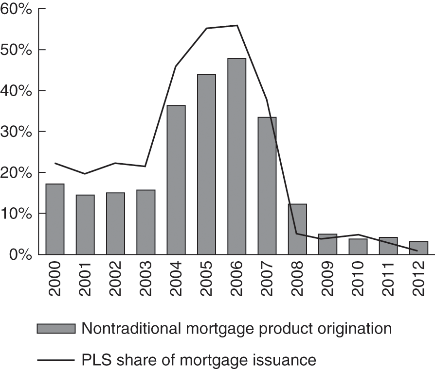
Figure 12.1 Market Share in Dollars of Nontraditional Mortgage Products and Private Label Securitization, 2000–2012
Note: Nontraditional mortgage products are subprime, Alt-A, and home equity loans.
While most conforming mortgages were securitized by Fannie Mae and Freddie Mac, most NTMs and subprime loans were securitized in the PLS market. Figures 12.1 and 12.2 (which disaggregate mortgages by type) show the share of PLS and NTM and subprime mortgage issuance peaking during 2006 and almost disappearing after 2008. While the PLS market share rose during the housing boom, the GSE (conventional, conforming) and Ginnie Mae markets shares shrank (Wachter Reference Wachter2014).
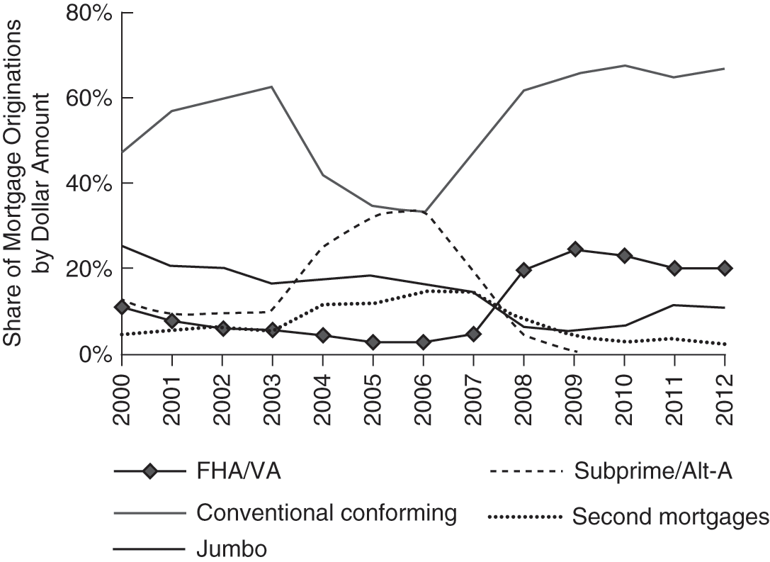
Figure 12.2 Origination Shares by Mortgage Type, 2000–2012
12.2.B Principal-Agent Problems in Securitization
Securitization ushered in new principal-agent problems that the inventors of MBS worked to address. Adverse selection was one issue, consisting of the fear that originators would retain their best loans and securitize the rest. Investors were also concerned about information asymmetries, because lenders know more about the quality of the loans they originate than investors and have incentives to conceal negative information when selling those loans.6
Private capital would shun the mortgage finance system absent assurances to investors on both scores. Consequently, securitizers used a host of techniques to address the principal-agent problems in securitization, including disclosures, underwriting standards, quality control, due diligence reviews, and risk retention. Key among those techniques was representations and warranties, the focus of this chapter.
12.2.C The Use of Representations and Warranties in MBS
Every mortgage-backed securitization starts out with the sale of a pool of mortgage loans by a seller to a purchaser. The purchaser is generally a GSE, an FHA/VA securitization issuer, or an investment bank that plans to transfer the loans to a special purpose vehicle for bundling into MBS for sale to investors. Often the seller is the originator, but it can also be a large bank that aggregates loans bought from a third-party originator. In the course of the series of transfers that make up a securitization, many of the transferors make representations and warranties to the next transferee down the chain (Murphy Reference Murphy2012).
The central contract governing the loan sale is a Mortgage Loan Purchase Agreement between the seller and the purchaser (Miller Reference Miller2014, 259, 267). This agreement or its equivalents are found in all three major securitization channels, including Ginnie Mae, the GSEs, and private-label securitizations (FHFA 2012, 6, 10–12). The typical agreement contains more than 50 representations, warranties, and covenants by the seller to the purchaser (see, e.g., Master Loan Purchase Agreement 2005, § 5 & Exh. A). The representations and warranties inure to the benefit of the purchaser and sometimes to its assignees, transferees, or designees, including the trustee of the securitization trust (see, e.g., id., § 6).
While these representations and warranties share common subject matters, in PLS transactions their precise language varies (sometimes significantly) across deals (Standard & Poor’s 2013b; Tate 2016). In contrast, representations and warranties are standardized for GSE and Ginnie Mae securities. The representations and warranties made to Fannie and Freddie are cheaper to litigate by virtue of their standardization and are also generally stronger than those agreed to in private-label deals (Fleming Reference Fleming2013; Strubel Reference Strubel2011).
Representations and warranties serve dual functions: deterrence and compensation. One reason investors demand those representations is to deter lax loan underwriting by lenders. Investors also require those provisions to assure compensation in the event of breach. For this reason, the enforcement provisions of the Mortgage Loan Purchase Agreement require repurchase of any mortgages that are found to be in breach.
12.2.C.1 The Contractual Representations and Warranties
Some representations and warranties deal with the legal status, bona fides, operating systems, and condition of the seller and related parties (see, e.g., Master Loan Purchase Agreement 2005, § 5(b) & Exh. A), but most involve statements about the legality and quality of the loans being sold. The loan-specific representations and warranties can be grouped into the following subjects (see, e.g., id., Exh. A; Miller Reference Miller2014, 270–73):
Mortgage Loans as Described: Under this provision, the seller affirms that information relating to the mortgage loans in the pool is complete, true, and correct and the interest rates are those stated in the mortgage notes. A related provision states that all necessary documents have been delivered to the custodian and that the seller possesses the complete, true, and accurate mortgage file.
Current Payment Status: In this representation and warranty, the seller confirms that no loan in the pool is in default or has been delinquent for 30 days or more in the past 12 months. In addition, a warranty provides a safeguard against early payment default by stating that the first three monthly payments shall be made within the month in which each payment is due. In a related, open-ended provision, the seller confirms that it has no knowledge of any circumstances or conditions that would cause any of the mortgage loans to become delinquent.
Legality: Representations and warranties typically provide that each mortgage loan when it was made complied in all material respects with applicable local, state, and federal laws, including, but not limited to, all applicable predatory and abusive lending laws. In addition, the seller warrants that none of the mortgage loans were “high cost” or predatory loans for purposes of federal or state or local anti-predatory lending laws. A companion provision states that the origination, servicing, and collection practices used with respect to the mortgage loans are legal and in accordance with accepted practices.
Appraised Value: Another group of representations and warranties provides that the properties securing the mortgage loans have been appraised according to the standards specified in the Mortgage Loan Purchase Agreement.
No Misrepresentations: This provision states that no one has engaged in any misrepresentation, negligence, fraud, or similar occurrence with respect to a mortgage loan.
Loans Meet Agreed-Upon Underwriting Standards: In this set of provisions, the seller confirms that the mortgage loans in the pool all meet specified underwriting standards, including maximum loan-to-value ratios and minimum credit scores.
Loans Meet Agreed-Upon Loan Features: In these provisions, the seller agrees that none of the loans in the pool contains prohibited features. This list of prohibited features varies with the loan pool, but sometimes includes balloon terms, negative amortization, shared appreciation, prepayment penalties, mandatory arbitration clauses, and/or single premium credit insurance terms.
Mortgage Loan Fully Marketable and Enforceable: These representations and warranties provide assurance that the mortgage loans are fully marketable and enforceable and have not been impaired, waived, or modified.
No Outstanding Charges: Here the seller states that all taxes, assessments, insurance premiums, and other charges due under the terms of the mortgages have been paid and are up to date.
Underlying Properties Intact and Adequately Insured: In this representation and warranty, the seller confirms that all of the properties securing the mortgage loans are undamaged and have adequate hazard insurance, including flood insurance where required, as well as title insurance.
Conforming Asset Class: This representation and warranty states that all of the mortgaged properties securing the loan pool belong to the appropriate asset class (e.g., residential properties instead of commercial properties).
Owner-Occupied: The seller affirms that all of the homes securing the loans are owner-occupied.
Provisions Regarding the Timing, Amount, and Crediting of Payments: Several other representations and warranties address the timing, amount, and crediting of payments.
Taken together, these representations and warranties allocate the responsibility for loan quality to the originator or other seller, who can ensure that quality more cheaply than the purchaser (Miller Reference Miller2014, 263, 286–88, 290).
Despite the wealth of representations and warranties, most put-back requests and disputes turn on a handful of core representations (271–73). These representations include statements that the loans in the pool: (1) are as described (particularly with respect to loan-to-value ratios, credit scores, debt-to-income ratios, owner-occupied status, and the like); (2) have no past delinquencies and will not go delinquent within the first three months after origination; (3) are free from misrepresentations; (4) are legal; and (5) conform with the agreed-upon underwriting standards. In addition, some repurchase requests are prompted by claims of inflated or fraudulent appraisals.
12.2.C.2 Enforcement Provisions for Representations and Warranties
The standard Mortgage Loan Purchase Agreement limits the contractual relief for breach of these representations and warranties to one set of remedies and one set alone7 (Miller Reference Miller2014, 274–76). Under the “Repurchase Obligation” provisions in versions of the Agreement before the crisis, if the substance of any representation and warranty was inaccurate and the inaccuracy materially and adversely affected the value of the mortgage loan in question or the interest of the purchaser, then the representation and warranty was breached, even if the seller was unaware and could not have been aware of the inaccuracy when the representation was made (see, e.g., Master Loan Purchase Agreement 2005, § 6). The Agreements go on to state that following prompt written notice of the discovery of such an inaccuracy, the seller shall use its best efforts to promptly cure the breach within 90 days. If the breach cannot be cured, then the seller, at the purchaser’s option, shall repurchase the mortgage loan at issue at the purchase price8 (see, e.g., id., § 6). Effectively, this gives the purchaser a put option for loans that violate representations and warranties.
In theory, this put option is quite strong. This remedy is not technically conditioned on a realized loss to the investor; instead, it can apply so long as a breach results in a material paper loss to the mortgage loan in question. As a practical matter, however, operationally relatively “small” errors in representations would not in general lead to exercise of the put option prior to default. In default, such errors become salient. And in the crisis, the decline in real estate prices made such ordinarily ignored errors particularly salient as prices and collateral declined dramatically.
At the same time, the contractual remedy for breach of representations and warranties is only as good as a seller’s solvency. For the put option to have bite, a seller must still be operating and have sufficient assets to pay a judgment. This became a particular concern in the case of breaches by nonbank lenders, more than 100 of whom operated with razor-thin margins and capsized after they lost their funding in 2007.9
12.2.D The Mortgage Crisis
Had investors given representations and warranties scant credence when they originally bought loans, those provisions might not have mattered. However, investors took representations and warranties seriously. The rating agencies, for instance, touted their review of the representations and warranties for every private-label deal in order to give investors confidence that their ratings had integrity (see, e.g., S&P Global Ratings 2004). After the crisis, the Basel Committee and government investigators concluded that investors had placed undue faith in the efficacy of representations and warranties (Basel Committee on Banking Supervision 2011; Ergungor Reference Ergungor2008).
To investors’ chagrin, those representations and warranties failed to prevent the spike in mortgage loan defaults that culminated in the 2008 financial crisis. As discussed earlier, by the early 2000s, private-label securitization had outgrown its traditional function of funding jumbo conforming loans to also financing increasing numbers of nontraditional mortgage products. From 2004 through 2007, investors flocked to subprime and Alt-A MBS because of their higher yields (McCoy et al. Reference McCoy, Pavlov and Wachter2009, 496–97 and fig. 1). Originators met the demand for higher coupon mortgages with risky interest-only and pay-option mortgages with no or negative amortization, which together reached an astonishing 50 percent of all mortgage originations in spring 2005 (id., 497, fig. 1). A series of decisions by federal banking regulators to deregulate residential mortgages also helped pave the way for this unprecedented growth (Engel and McCoy Reference Engel and McCoy2011, 151–205).
During the run-up to the crisis, the proliferation of subprime and Alt-A loans was accompanied by a marked deterioration in loan underwriting standards. Between 2002 and 2006, two of the strongest predictors of default rose noticeably: loan-to-value ratios and the proportion of loans with combined loan-to-value ratios of more than 80 percent (Levitin and Wachter Reference Levitin and Wachter2015). Meanwhile, lenders increasingly layered one risk on top of another, often combining low-equity, no-amortization loans with reduced documentation underwriting (McCoy et al. Reference McCoy, Pavlov and Wachter2009, 504–05 and fig. 3). Loan fraud also became more prevalent during this period, with private-label securitized mortgages and low-documentation mortgages experiencing particularly high levels of fraud (Mian and Sufi Reference Mian and Sufi2015). Loan origination volume shifted to lenders who used private-label securitization with lower and less well-enforced underwriting standards, although there is evidence that there was somewhat of a decline in the GSE underwriting standards as well (Wachter Reference Wachter2014, Reference Wachter, Wachter and Tracy2016). Under pressure to maintain market share, other lenders cast aside their reputational concerns and lowered their lending standards in response (Engel and McCoy Reference Engel and McCoy2011, 38–40).
As the ensuing disaster unfolded, it soon became apparent that representations and warranties had not prevented the sharp deterioration in underwriting standards during the credit bubble. Increasingly, it became apparent that loan features and performance that were in direct breach of the representations and warranties – including excessive loan-to-value ratios, early payment defaults, and outright fraud – had become commonplace. The first warning signs of higher defaults appeared in subprime and Alt-A adjustable-rate mortgages (ARMs) beginning in mid-2005 and worsened after that (see Table 12.1). As defaults mounted in 2006, the number of mortgage repurchase requests remained modest but started to increase in response10 (Sabry and Schopflocher Reference Sabry and Schopflocher2007). According to Fitch Ratings, early payment defaults were the “root cause” of these early repurchase requests, particularly in loans with layered risks such as lower credit scores, second liens, and stated income underwriting (Fitch 2006).
Table 12.1: Percentage of Subprime and Alt-A Adjustable Rate Mortgages (ARMs) 90 Days or More Past Due or in Foreclosure
| Reporting Period | Subprime ARMs | Alt-A ARMs |
|---|---|---|
| July 2005 | 5.63% | 0.43% |
| July 2006 | 8.16% | 0.74% |
| July 2007 | 14.63% | 3.06% |
| December 2007 | 20% | 6% |
Through 2006, rising housing values allowed troubled borrowers to refinance their mortgages in order to avoid default. In the first quarter of 2007, however, housing prices began to slide nationwide for the first time since the Great Depression and the foreclosure crisis began in earnest. During this period, the compensatory and deterrent functions of representations and warranties were seriously tested.
12.2.E Repurchase Demands and Actions to Enforce Put-Back Clauses
As falling home prices impeded the ability of distressed borrowers to avoid default by refinancing their loans or selling their homes, mortgage delinquencies skyrocketed and mortgage put-back requests surged (Hartman-Glaser et al. 2014, 28, fig. 3). Data on aggregate recoveries for all put-back demands are hard to come by. But we can get a sense of the magnitude by examining put-back collections by Fannie Mae and Freddie Mac.
The two GSEs sought recourse for bad loans for two lines of business activities. First, Fannie Mae and Freddie Mac lodged repurchase claims against originators or aggregators for defective loans that had been sold to them. While the evidence is incomplete, the percentage of loans subject to Fannie/Freddie buyback claims seems to have been modest (less than 2 percent of balances at origination for GSE 30-year, fixed-rate full-documentation, fully amortizing loans from select deals) (Goodman and Zhu Reference Goodman and Zhu2013; Goodman et al. Reference Goodman, Parrott and Zhu2015, 3–5 and fig. 1). From January 1, 2009 through the third quarter of 2015, as a result of those claims, Fannie and Freddie collected a total of $76.1 billion from more than 3,000 companies for loans repurchased from their mortgage-backed securitization trusts (GSE Repurchase Activity). This more than doubled the total industry liability that Standard & Poor’s had originally estimated for GSE repurchase and securitization claims in 2011 (Murphy Reference Murphy2012). Not all of the GSEs’ put-back claims were successful, however, and the two enterprises ultimately withdrew or stopped pursuing another $61.9 billion in repurchase demands (GSE Repurchase Activity). For the put-back claims that settled, the average payment per loan was substantially less than the average purchase price for all of the loans11 (Siegel and Stein Reference Siegel and Stein2015).
In addition, Fannie and Freddie pursued claims for their purchases of private-label MBS during the housing bubble (Hill Reference Hill2011/2012, 375–81). In January 2016, their regulator and conservator, the Federal Housing Finance Agency (FHFA), reported that it had settled lawsuits against 16 out of 18 financial institutions involving the sale of private-label instruments to Fannie and Freddie. Technically, these were not buyback claims insofar as the actions alleged securities law violations and sometimes fraud in the sale of the PLS. But these claims were also founded on lax mortgages and their financial effect on originators and issuers was similar. Total settlement amounts equaled $18.2 billion as of year-end 2014 (FHFA 2016b).
12.2.E.1 Sources of Put-Back Claims
As this discussion of GSE recoveries suggests, each of the three securitization channels has generated put-back demands and lawsuits (Standard & Poor’s 2013a). While these demands share many similarities across channels, there are also differences depending on the channel.
Turning to the private-label channel, many private-label issuances featured long chains of transfers involving mortgage brokers, loan originators, correspondent or wholesale lenders, investment banks, depositors, trustees, and investors. At each link in the securitization chain, representations and warranties were often made. Consequently, put-back demands for any given securitization in the PLS channel usually involved not just one, but a sequence of repurchase requests throughout the chain12 (Hill Reference Hill2011/2012, 375; Murphy Reference Murphy2012). Private-label securities were especially prone to buyback claims because they experienced higher average default rates than GSE RMBS (Fitch 2011).
As discussed, the GSE channel also generated repurchase claims. Although the GSEs’ issuances performed better on average than their PLS cousins, as noted previously, the representations and warranties made to Fannie and Freddie were stronger in nature and spawned more interpretive case law due to their standardization, making them easier to litigate successfully (Fleming Reference Fleming2013; Strubel Reference Strubel2011).
Finally, defective FHA-insured loans generated their own set of buyback and statutory claims, sometimes by Ginnie Mae and sometimes by the U.S. Department of Justice (DOJ). Some of those claims became turbocharged due to certifications that the originators had to sign when making FHA-insured loans. Under the FHA’s direct endorsement program, designated lenders are allowed to designate mortgages as eligible for FHA insurance. In order to qualify for this program, lenders must provide annual certifications that their quality control systems comport with all relevant rules of the Department of Housing and Urban Development (HUD)13 (Goodman Reference Goodman2015). Lenders must further certify that each FHA-insured loan observes all relevant HUD rules14 (id.). Before 2015, lenders had to make these affirmations regardless of their knowledge or their ability to detect violations (id.).
The DOJ has taken the position that any lender who knowingly submits loans for FHA mortgage insurance containing material underwriting defects that disqualify those loans for FHA mortgage insurance makes a false claim for purposes of the False Claims Act (U.S. Department of Justice 2016). Under that Act, lenders who knowingly submit false or fraudulent claims to the federal government for payment or approval are liable to the government for damages. Justice Department claims under the False Claims Act pose the highest monetary exposure of any of these types of claims because violators must pay civil penalties of $5,000 to $11,000 per claim plus treble damages. In 2011, the United States sued all of the top five mortgage originators for False Claim Act violations in connection with their certifications for FHA insurance15 (Goodman Reference Goodman2015). According to the Justice Department, the federal government recovered more than $5 billion in these and other claims for housing and mortgage fraud from January 2009 through October 2015 (U.S. Department of Justice 2015).
In addition, the DOJ has also pursued Federal Housing Administration claims under the powerful and flexible civil money penalty provisions in Section 951 of the Financial Institutions Reform, Recovery and Enforcement Act of 1989 (FIRREA) (Standard & Poor’s 2013a). FIRREA is attractive in many circumstances because it has a longer limitations period and lower threshold of proof than the False Claims Act. However, the Second Circuit Court of Appeals cast doubt on the viability of this theory when it ruled in 2016 that FIRREA precludes recovery for intentional breach of contractual representations and warranties through the sale of poor-quality mortgages absent evidence that a seller intended to defraud purchasers when the representations and warranties originally were made (United States ex rel. Edward O’Donnell 2016).
12.2.E.2 Success of Put-Back Claims
As the GSE experience shows, buyback claims have not been invariably successful. The chances of prevailing on claims for breach of representations and warranties vary widely according to the type of breach, the passage of time, the litigation capacity of the plaintiff, and the solvency of the defendant.
To begin with, success may turn on the type of claim. Some breaches of representations and warranties are easily proven because they turn on commonly available evidence using objective standards. Early payment defaults are a good example, because servicing records normally show whether the borrower was delinquent in the first three months of the loan.
Other breaches are harder to substantiate and subject to dispute. The facts may require further investigation into hard-to-obtain documents outside of the purchaser’s possession or the representation in question may be couched in vague or subjective language. Thus, cases alleging false loan-to-value ratios or appraised values require reconstructing the actual appraised value at origination, which is subject to debate and difficult to do. Purchasers who assert other types of fraud or misrepresentation generally must prove those claims based on evidence from the face of the loan or deal documents, which can be daunting (Miller Reference Miller2014, 300–01). Buyback disputes over loans that supposedly were allowed to depart from underwriting standards due to compensating factors can be particularly messy to litigate.
While it is relatively simple to point to errors in loan documents based on a sample of the contested book of business, the import of those errors will be in question. Were they simple errors (such as whether the borrower was self-employed versus a contractual employee) that would not or should not be counted against the originator? Or is a large share of such errors indicative of sloppy underwriting that should and does matter to outcomes in conjunction with a price decline, even though it is the price decline itself that is a major factor in default and thus in losses?
In addition, the amount of time that has elapsed since the loan sale affects the deterrent role of representations and warranties and the prospects for compensation. Many Mortgage Loan Purchase Agreements predating the crisis contained no hard-and-fast outer time limits on bringing put-back claims. Under those contractual provisions, and absent an otherwise binding statute of limitations, a purchaser could ostensibly demand repurchase at any time upon discovery of a breach of a representation until the loan principal was fully repaid (Hartman-Glaser et al. 2014; Miller Reference Miller2014, 311; Tate 2016). This is not a hypothetical concern: Hartman-Glaser and colleagues (2014, 2 n. 2) discovered loans from GSE securitizations going back to 1985 that were the subject of repurchase requests between 2011 and 2014. In too many cases, defects did not surface and repurchase claims were not made until those responsible were long gone, eviscerating the deterrent function of representations and warranties.
This timing issue is a double-edged sword for purchasers and sellers. The more time that elapses until a put-back demand is made, the harder it is for the purchaser to prove due to dimming memories, missing witnesses, and lost documentation (Miller Reference Miller2014, 299–300). At the same time, the specter of open-ended contingent liabilities can erode investors’ confidence in a bank or other issuer. For this reason, sellers have aggressively resisted older put-back claims based on lack of reasonably prompt notice16 or expiration of statutes of limitations (id.).
The litigation capacity of the purchaser also affects the likelihood of successful put-back claims. The vigor with which the GSEs pursued buyback demands reflected their ability to terminate lenders’ contractual rights to sell agency loans (Hill Reference Hill2011/2012, 371),17 their greater litigation might combined with that of the federal government, plus the mission of Fannie and Freddie’s conservator to maximize the assets in the conservatorship estates in many cases. Similarly, Ginnie Mae’s ability to pursue claims through civil actions brought by the Justice Department – together with the threat of treble damages under the False Claims Act – substantially enhanced its power to negotiate favorable settlements.
In contrast, investors found it harder to bring successful put-back claims for private-label securities. One hurdle is that representations and warranties for PLS are less standardized than those for agency MBS (Fleming Reference Fleming2013; Standard & Poor’s 2013a, 6). In addition, in order to have standing, at least 25 percent of an issue’s shares must first typically vote to demand that the securitization trustee pursue a put-back claim. Only if the trustee fails to take action within a set period of time may investors directly sue. Still, investor groups have managed to surmount this obstacle (Murphy Reference Murphy2012; Standard & Poor’s 2013a, 6).
Finally, as noted before, recovery depends on the seller’s continued solvency. The largest banks survived years of repurchase claims bruised but intact (Standard & Poor’s 2013a, 3, 7–8). However, other mortgage originators failed due in part to high put-back demands (Barr Reference Barr2007; New Century Bankruptcy Court Examiner 2008, 36, 70–72, 105–06, 405–06), leaving some of those demands unsatisfied.
12.3 Market Responses and Policy Implications
There have been two major market responses to the post-crisis impact of put-backs. First, citing the need to avoid future put-backs (Lux and Greene Reference Lux and Greene2015, 17, 24), major lenders – particularly well-capitalized lenders who have much to lose in the event of future put-back claims – have either withdrawn from government-insured lending or have imposed on themselves credit overlays that go beyond the requirements of the GSEs, thereby lowering their market share.18 Second, nonbank lenders have emerged as the major origination channel to fill this gap. The shift is dramatic.
The problems with these market responses are twofold. First, the shift to thinly capitalized entities implies that, in a future crisis, representation and warranty penalties could not be effectively enforced against those entities. This undermines the compensatory value of representations and warranties going forward, as well as deterrence.
Second, lenders who believe they are no longer assured of default insurance through FHA and the GSEs are imposing credit overlays that go beyond the levels required by FHA and the GSEs. These lending constraints go beyond historic levels and beyond the levels historically associated with creditworthy lending, with mortgage market and home lending consequences that are described later.
12.3.A The Shift to Thinly Capitalized Entities, Growth of Credit Overlays, and Consequences
Immediately after the crisis, most home mortgages were originated by the major banks that were subject to capital adequacy and repurchase reserve requirements. More recently, however, the market share of mortgage originations by banks and especially the largest banks has fallen substantially (see Figure 12.3).19 This void has been filled by more thinly capitalized nonbank mortgage originators who are not regulated by prudential banking regulators for solvency (Lux and Greene Reference Lux and Greene2015), renewing concerns about the financial capacity of those lenders to make good on their representations and warranties.
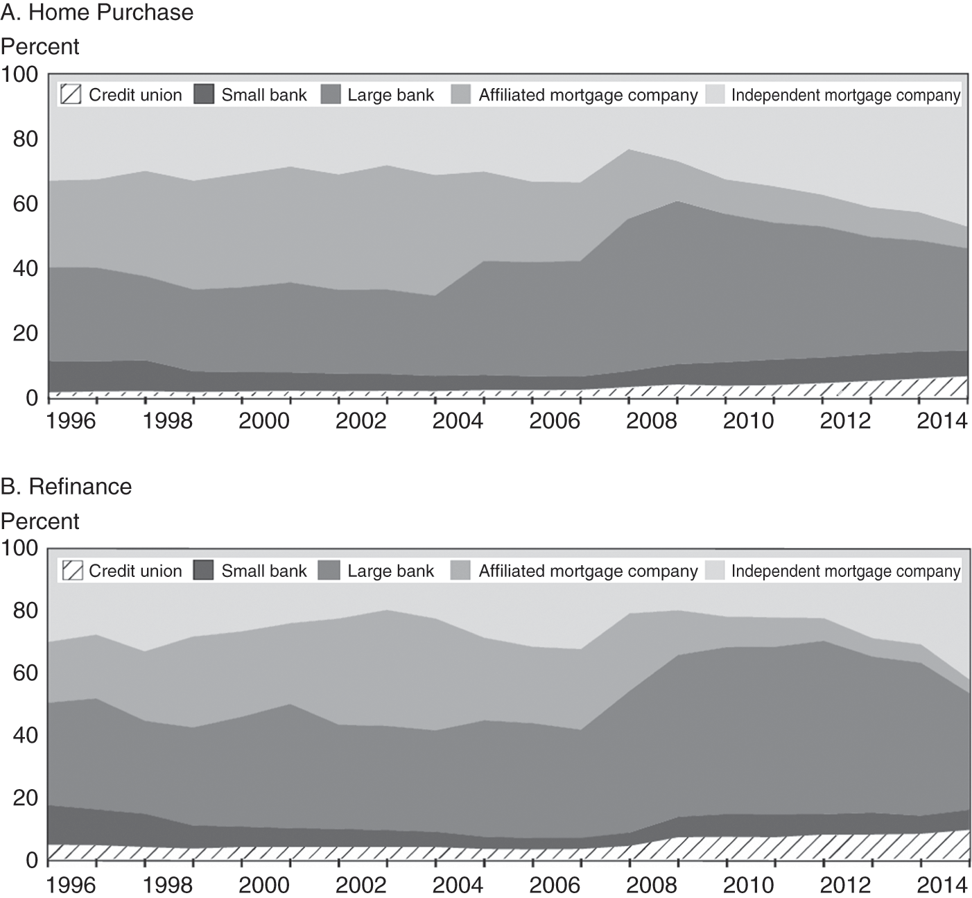
Figure 12.3 Market Share by Lender Type, 1995–2014
The lack of willingness on the part of established, traditional banks to extend mortgage credit has created an opportunity for a new type of market participant: minimally capitalized nonbank mortgage lenders. These lenders are denoted in Figure 12.3 as independent mortgage companies. In view of the recent history of successful repurchase litigation against banks, nonbank lenders enjoy a distinct competitive advantage because they lack legacy put-back exposure and have scant capital at risk for future repurchase claims. The growth of these institutions (Standard & Poor’s 2014) presents unique systemic risk – as these lenders are not subject to traditional capital requirements under prudential bank regulation and are minimally capitalized,20 their failure can be harmful to the market as a whole (FHFA OIG 2014b, 23–24; FSOC 2015, 10, 114). There is no evidence, moreover, that investors are demanding pricing differentials based on the capital adequacy of individual sellers (Standard & Poor’s 2013a).
At the same time, imposition of credit overlays by bank lenders who believe they are no longer assured of default insurance through FHA and the GSEs has resulted in a mortgage market that is notably constrained. This market constraint may be explained in part from regulatory pressures from HUD and DOJ. Although the primary intent of HUD and DOJ enforcement is compliance with HUD rules, it has prompted FHA’s largest bank lenders to announce that they are significantly reducing their extension of mortgage credit in response (Goodman Reference Goodman2015). As Goodman states, “lenders have begun to protect themselves the only way available to them: credit overlays, risk-based pricing, or a general pull away from FHA lending” (id.).
As evidence of the role of buyback requests on mortgage underwriting standards, Hartman-Glaser and colleagues (2014) show that the change in the probability of buyback requests on GSE MBS explains tighter mortgage lending standards. Figure 12.4 demonstrates the tightening of standards for FICO scores.
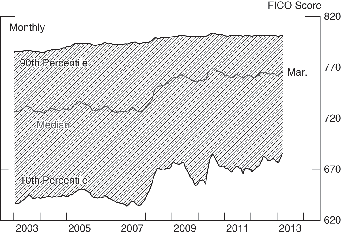
Figure 12.4 FICO Credit Scores on New Prime Purchase Mortgages from 2003 to 2013
The housing market has certainly made a recovery since the financial crisis, with housing starts having doubled since the recession. However, these heightened constraints on mortgage credit continue to suppress demand for housing and homeownership21 (Zandi and Parrott Reference Zandi and Parrott2014). In an analysis of the extent to which constrained credit has affected the mortgage market, Bai and colleagues (Reference Bai, Goodman and Zhu2016) found that 5.2 million more residential mortgages would have been made between 2009 and 2014 if credit standards had been at levels similar to those in 2001.
The tightening of the availability of credit has implications for homeownership. Acolin and colleagues (Reference Acolin, Bricker, Calem and Wachter2016a) estimate the role of the tightening of credit on the aggregate homeownership rate. They find that the homeownership rate in 2010–2013 is predicted to be 5.2 percentage points lower than it would be if borrowing constraints were at the 2004–2007 level and 2.3 percentage points lower than if the constraints were at the 2001 level, before the relaxation of credit took place (Acolin et al. Reference Acolin, Bricker, Calem and Wachter2016b, 13).
This tightening in lending standards is part of a cycle in lending. During the credit expansion leading up to 2008, representations and warranties contributed to the overheating of the cycle by giving false assurance to investors while failing to deter the race to the bottom in lending standards. Years later, the protracted enforcement of representations and warranties slowed recovery from the crisis by impeding access to mortgages for creditworthy borrowers. This history of under-correction during the bubble and over-correction following the collapse is the hallmark of procyclicality.
This procyclicality has micro- and macro-prudential repercussions as well as serious distributive implications. The after-the-fact use of representations and warranties as a means to allocate risk presented solvency threats to individual entities as well as having macro repercussions, by increasing systemic risk and slowing recovery. The distributive implications of the unnecessarily tight credit box on low- and moderate-income households and people of color persist.
Accordingly, the goal of reforms to representations and warranties should be to reverse the procyclicality that is inherent in the current system. To achieve this, it will be necessary to right-size the enforcement of these provisions while endowing them with deterrent effect. Doing so will enhance financial stability while expanding the credit box in a healthy and sustainable way going forward.
12.3.B Procedural Reforms
One way to increase the efficacy of representations and warranties is to counter the long temporal disconnect between breaches of those representations and enforcement. In many cases, the perpetrators of those breaches were long gone by the time repurchase claims were made. Shortening the timespan between the sale of loans and the presentation of put-back claims will enhance deterrence while speeding up recovery.
After the financial crisis, the put-back process was slow to initiate in many cases and arduously protracted afterward, thus prolonging the threat of litigation. In part, this could be blamed on resistance to put-back claims by sellers. However, purchasers contributed to the drawn-out nature of the proceedings by dragging their feet in presenting claims. The GSEs, for instance, did not close out their repurchase claims on loans originated before 2009 until the end of 2013, and only then at the insistence of FHFA’s then acting director, Edward DeMarco (Goodman et al. Reference Goodman, Parrott and Zhu2015, 7).
The GSEs, FHFA, and other actors eventually instituted a variety of reforms to speed up the put-back process. The GSEs instituted sunset provisions to bring some finality to the put-back process for performing loans.22 In addition, some court decisions hold that statutes of limitation on buyback claims run from the date of sale, not the date of discovery (Miller Reference Miller2014, 290, 312), putting the onus on purchasers to make claims more promptly.
Another concern is the vague and open-ended nature of some of the representations and warranties on which sellers are sued. In private-label deals, sellers had latitude to renegotiate the language of the representations and warranties they agreed to, thus potentially undermining their capacity to deter. Their negotiating ability was substantially less in deals with the GSEs and Ginnie Mae.
There will always be tension about the advisability of objective representations versus ones that are more general and ambiguous. Sellers want certainty about compliance and the extent of their exposure; purchasers worry about losses from negligence, fraud, and misconduct that they cannot anticipate in advance. A problem, as discussed further later, is that a breach may be “minor.” In the nature of underwriting it may be difficult to avoid such mistakes completely. Then in the aftermath of a crisis, all such mistakes may be grist for put-back claims. But how to tell which claims are important and which are not? While this tension will likely never fully be resolved, the following principles can be used to cabin the open-ended nature of certain representations and warranties:
First, the industry should adopt improved procedures to expedite the negotiations over put-back claims. Sellers have complained that purchasers insist on repurchase even when loans go delinquent due to life events such as job loss and divorce following origination (Standard & Poor’s 2013b). It goes without saying, however, that sellers should not be responsible for events such as these outside of their control unless breach of a representation or warranty exacerbated the loss severity or risk of default. To resolve these and similar repurchase disputes without resort to litigation, sellers and purchasers could agree to send those disputes to neutral third-party arbitration. The GSEs adopted this independent dispute resolution procedure in 2016 (FHFA 2016a; Standard & Poor’s 2016) and Ginnie Mae and private-label conduits might follow suit.
Second, loans that consistently perform for a stated number of years should be exempt from repurchase claims. The GSEs’ sunset provisions embody this approach by shielding loans with a 36-month record of on-time payments (12 months in the case of HARP loans) from buyback demands (FHFA OIG 2014a, 15–17; Goodman et al. Reference Goodman, Parrott and Zhu2015, 3).
Third, liability for breach should be excused where the seller was not aware of the problem and could not have discovered it using reasonable investigation. HUD revised its annual certification in this respect in 2015 by adding the language “to the best of my knowledge and after conducting a reasonable investigation” (Goodman Reference Goodman2015).
It would be also advisable to standardize representations and warranties as much as possible in the private-label market. Doing so would promote the growth of arbitral decisions and case law interpreting those standardized terms, which could then provide guidance for faster resolution of similar disputes in the future.
Similarly, it is time to confront the fact that False Claims Act treble damages sanctions are overkill in the absence of knowing fraud. The threat of treble damages is discouraging bank lenders from serving the low- and moderate-income community that FHA loans were designed to serve. Instead, penalties for flaws in FHA loans should be tailored to the FHA’s defect taxonomy, according to the seriousness of the violation and the violator’s culpability (Goodman Reference Goodman2015; HUD 2014).
In an ideal world, the deterrent effect of representations and warranties could also be strengthened on the front end to curb the proliferation of lax loans during credit booms while obviating the need for enforcement. Suggested reforms have included improved due diligence and internal quality control, stronger data integrity controls for automated underwriting systems, faster post-purchase reviews by investors, and improved, standardized disclosures for put-back obligations (which the Securities and Exchange Commission issued in 2014 (Dodd Frank Act § 943; SEC 2014)).
All of these reforms, in place or contemplated, have a potential flaw, however, which is that they rely on originators’ compliance. Standardized disclosures and detailed underwriting guidelines are only as good as the integrity of the underwriting process that generates them. Even if some purchasers carefully monitor loan originations through pre-purchase and post-purchase quality assurance and control as suggested, there is the potential for other purchasers to not do so, thus undermining the quality of underwriting for the system as a whole. Those originators and purchasers who skirt requirements and procedures in the “hustle” for business will rapidly gain market share, even as they lower their costs. The result will be higher prices as loans are made that otherwise would not be made and the higher prices will mask the poor underwriting. The representations and warranties may stop some, but if more aggressive lenders operate in this way, there is an “externality” (Wachter Reference Wachter2014) that results as the quality of the aggregate mortgage book of business deteriorates and risk increases even for more careful lenders. Moreover those lenders who are willing to undermine standards will set the bar lower for other lenders who unless they similarly lower the bar will not be able to attract the marginal borrower (Pavlov and Wachter Reference Pavlov and Wachter2006). And the process is unleashed again.
12.3.C Systemic Reforms
Lenders have called for greater clarity in the representations and warranties that they provide. But better drafting alone is not the answer to deterrence. The events of 2008 showed that lenders ignored even objective representations and warranties such as loan-to-value caps in the rush for greater market share at the height of the credit bubble. The market incentives are for contractual representations and warranties to be procyclically implemented. No one will exercise a put option when prices are rising, but everyone will do so once they have fallen. Besides market forces that lead to sliding standards across firms during the bubble, in the aftermath, there will be competitive tightening: firms will not want to be the lax lender when they fear that representations and warranties will be strictly enforced. While a normal level of “mistakes” is to be expected and not entirely avoidable, such mistakes will become the potential source for put-backs if in the overall market, prices have plummeted due to the aftermath of the unsustainable expansion of credit. And at that point put-backs bite. Accordingly, stronger external measures are needed in order for representations and warranties to have real teeth, to prevent market-wide pressures for deterioration in underwriting. Some of those measures are already in place.
Ability-to-Repay and Qualified Mortgage Provisions: The new ability-to-repay and qualified mortgage rule promulgated by the Consumer Financial Protection Bureau places a federal floor under underwriting practices by prohibiting reduced documentation loans. Because the rule requires documentation and verification of income and assets, it should significantly reduce one of the main sources of put-back claims. In addition, the rule creates a new category of loans with especially risky features such as balloon terms and negative amortization – called non-qualified mortgages – and imposes liability for any such loans made in disregard of the borrowers’ ability to repay (CFPB 2013; Dodd-Frank Act §§ 1411–1412). The rule is enforced through federal examinations of lenders and through public and private enforcement mechanisms (which apply to poorly underwritten loans and non-qualified mortgages), which should help ensure that the federal floor is observed (Dodd-Frank Act §§ 1024(a)(1)(A), 1025–26, 1042(a), 1413, 1416(b)).
Heightened Solvency Safeguards: Increased solvency supports would give lenders a greater stake in observing representations and warranties ex ante in order to avoid liability for breach ex post, while providing purchasers with greater assurance of compensation where needed. These supports can take the form of capital requirements, provisioning thresholds, and mandatory risk retention.
To begin with, countercyclical provisioning requirements for representations and warranties would give representations and warranties more teeth while ensuring that the reserves on hand for compensation by lenders are sufficiently deep. Currently, insured depository institutions maintain reserves against their representation and warranty exposures. However, the computation of those reserves is severely procyclical. Because institutions compute these reserves based on losses already incurred, instead of expected future losses (FASB 2016, 1; Standard & Poor’s 2013a, 6), they chronically under-reserve for representation and warranty liability during expansions, while struggling to boost those reserves post-crisis once lawsuits spike.
A shift to the countercyclical technique known as dynamic provisioning would reverse this perverse sequence of events. During credit booms, dynamic provisioning triggers a switch in the algorithm for loss reserves that calculates those reserves as if credit were contracting. Later, if an economic downturn strikes, that switch is turned off (Caprio Reference Caprio2009, 22; Ren Reference Ren2011, 11–19). This model requires lenders to build up their representations and warranties reserves during credit booms, when they have cash, and allows them to spend down those reserves during economic downturns to pay for any legal exposures. To the extent that these added reserves made representations and warranties more effective, any resulting legal liability would be reduced.23
While federal regulators have not adopted dynamic provisioning, U.S. accounting standards have made strides toward countercyclical provisioning. In 2016, the Financial Standards Accounting Board adopted a new standard requiring lenders to calculate their loan loss allowances based on expected credit losses, regardless of whether losses have probably been incurred (FASB 2016, 1–2; see Board of Governors et al. 2016a). The provision, which takes effect in 2019, requires lenders to book all projected losses over the lifetime of the loans immediately upon origination. This is not a fully countercyclical approach because some losses for long-term residential mortgages may not become expected until years down the road. Nevertheless, the new provision will require lenders to incorporate forecasts of future conditions in addition to past and current events and record projected losses up front. Importantly, the new FASB provision applies to all bank and nonbank lenders alike.
Minimum capital requirements form another important solvency safeguard. Under Basel III, prudential banking regulators substantially increased the capital adequacy requirements for residential mortgages originated and securitized by federally insured depository institutions.24 In addition, Basel III imposes a countercyclical capital buffer designed to kick in when credit conditions start to overheat (Department of the Treasury et al. 2013, 62031, 62171). While questions surround the implementation and efficacy of the countercyclical capital buffer if left to regulators’ discretion (McCoy Reference McCoy2015, 1204–05 and n. 118), Basel III takes a step in the right direction by increasing the deterrence exerted by representations and warranties during incipient credit bubbles.
In the capital arena, however, regulatory arbitrage remains a serious concern. Federal banking regulators lack jurisdiction to impose minimum capital requirements on independent nonbank lenders (Board of Governors et al. 2016b, 37).25 Even if they did have jurisdiction, uniform capital standards would be highly unlikely, given federal regulators’ conclusion that Basel III is incompatible with the business models of some large nonbank mortgage servicers (id., 37–39). This means that as the nonbank sector grows, it will continue to enjoy arbitrage opportunities and escape the disciplining effect of uniform capital requirements. Not only will this reduce the in terrorem effect of representations and warranties, it will perpetuate competitive inequalities among bank and nonbank lenders. Unless Congress empowers federal banking regulators to impose capital adequacy requirements on mortgage lenders regardless of charter, it will be incumbent on the GSEs, Ginnie Mae, and the private-label sector to demand more meaningful safeguards from nonbank originators than they have so far.26 Whether these investors will impose sufficient capital requirements during a credit boom, when nonbank originators are likely to expand and investors are prone to over-optimism, is questionable. Moreover if investors and private-label securitizers themselves, in a bid to grow market share, fail to demand comparable safeguards from nonbank originators, the game will be on again. We can already see potential warning signs of trouble in the rising numbers of FHA mortgages being made by nonbank lenders to borrowers with FICO scores below 660 (Lux and Greene Reference Lux and Greene2015, 18–25).
12.4 Conclusion
During the run-up to the 2008 financial crisis, representations and warranties (contractual statements enforceable through legal action) on lending processes may have given investors false assurance that mortgage loans were being properly underwritten. This assurance in turn may have contributed to overinvestment in MBS in two ways. First, the assumption that legally enforceable penalties associated with representations and warranties would deter lax underwriting may have led to less screening of loans than would otherwise have occurred. In turn, the failure to oversee actual underwriting practices enabled the spread of lax lending practices. The existence of these representations and warranties and the potential penalties associated with them did not deter lax underwriting. Paradoxically, after the fact when the representations and warranties were enforced, this enforcement coincided with a tightening of credit beyond historic norms, with serious distributive implications. Post-crisis, lenders’ fears over put-back exposure appear to have caused them to scale back, particularly on government lending to creditworthy borrowers. The representations and warranties as used in mortgage lending in the run-up to the crisis were part of the procyclicality of lending, both in the easing and tightening phases of the lending cycle.
We suggest reforms to add to the deterrent value of representations and warranties. Particularly we suggest a shift to the countercyclical technique known as dynamic provisioning to increase the in terrorem effect of representations and warranties. This model requires lenders to build up their representations and warranties reserves during credit booms, when they have cash and when risk is growing, and allows them to spend down those reserves during economic downturns to pay for any legal exposures. To the extent that these added reserves signaled greater risk, they would make self-enforcement of representations and warranties more effective and procyclicality would be reduced. We also propose stricter capital standards.
Nonetheless, such changes would be useless unless they were adopted throughout the lending industry: otherwise, just those entities with risky practices would increase their market share. And next time such entities are more likely to be thinly capitalized, as the lesson of capital exposure to legal risk has been learned, thus further reducing the deterrence effect of representations and warranties, going forward.
Authors’ Note
Our thanks to Lee Anne Fennell, Benjamin Keys, Karen Pence, and the other participants at the conference sponsored by the Kreisman Initiative on Housing Law and Policy at the University of Chicago in June 2016 for their helpful comments.
The housing crisis of the 2000s exposed fissures in the U.S. financial system. These shortcomings allowed the system to become encumbered with excessive risk and ultimately triggered the worst economic downturn since the Great Depression. In the wake of the deep recession, many academics and researchers wrote post-mortems identifying key causes of the crisis. In 2010, Congress passed the Wall Street Reform and Consumer Protection Act, also known as Dodd-Frank, and President Obama signed it into law. It sought to address many of the identified problems by reforming regulations pertaining to mortgage lending, securities trading, banking, insurance, consumer protection, and corporate governance.
This chapter explores three causes of the crisis that the regulatory reforms have yet to fully address. First, we highlight challenges that prevented credit rating agencies from being a useful source of information for mortgage-backed securities investors to impose effective market discipline on issuers. Second, we show the failure of several institutional arrangements designed to prevent firm owners and managers from looting the institutions over the short run at the expense of shareholders, who are expecting a maximization of profits over the longer term. Finally, we consider markets from the consumer perspective. We note the tension between overcoming market tendencies to ration credit and exposing households with limited resources to risks associated with products that can broaden access to credit by easing borrowing constraints.
In each case, we offer possible strategies for more effectively tackling these problems. Regarding ratings agencies, we propose a new structure where agency-investor conflicts of interest are removed and agencies only assess “ratings eligible” products. Reforms in executive compensation, covenant banking for investment banks, and increased penalties for looting that make criminal liability a real deterrent for firm owners and managers are possible avenues to reduce the likelihood of looting by insiders. Third, we argue that significant investments should be made in financial education to make consumers an additional bulwark – to go with laws and regulations – against abuses and bad outcomes.
To begin, we tell the story of Black Friday, a deep financial crisis that occurred in the mid-nineteenth century. We take this historical approach because Black Friday shares many of the features that brought down the economy during the recent crisis, including the issues that we highlight. Indeed, a punchline of the current analysis is that many of the problems in the recent episode are enduring and inherent to virtually all regulatory structures. This fact should inform what we ask our regulations to address and how we define transparency in financial markets.
13.1 A Cautionary Tale of Undisciplined Markets
It was Wednesday evening in downtown Manhattan, and Jay Gould had a problem. He had just learned, through a secret letter written from the First Lady to her sister-in-law Virginia Corbin, that the president of the United States was “very much annoyed” by Gould’s speculation in the gold market and wanted him to unwind his positions immediately. “I am undone,” Gould said to Corbin’s husband, Abel, “if that letter gets out” to the public.
The date was September 22, 1869, and Gould had been buying gold since April. By himself, Gould didn’t have enough money to move markets, but in this era before securities regulation, he didn’t have to work alone. He formed a pool with some of the biggest investors on Wall Street and instructed them to push up the price of gold with their purchases. Meanwhile, he leveraged his position as the president of the Erie Railroad to borrow tens of millions of dollars and multiply his wager. He even paid President Ulysses S. Grant’s brother-in-law to lobby the government not to sell its gold reserves.
Now, it seemed, the president had caught on to his scheme.
The next morning, Gould started selling gold at the opening bell, but he didn’t tell all of his partners in crime. He feared a fire sale would ensue if everybody tried to exit at the same time, so he got out stealthily and let them keep buying unaware.
It took only a day for the market to figure out what he was up to. Sell orders came in so fast that the telegraph couldn’t keep up. “Nearly a thousand individual investors were bankrupted on the day’s activity,” writes Gould’s biographer Edward J. Renehan Jr. “Fourteen brokerage houses went under, along with several banks.” Henceforth, September 24, 1869, would be known as Black Friday (Renehan Reference Renehan2005).
We begin our story here because Jay Gould was arguably the first trader to stoke a speculative bubble on Wall Street, followed by a nationwide financial panic, using real estate as collateral. Railroads were the first great real estate companies in American history, gobbling up land to lay tracks across the country and building the biggest corporations the world had ever seen. In their manipulations and innovations, we see many parallels to the housing booms and busts in our own time.
But we also begin our analysis with the tale of Jay Gould because it evokes such a fitting reaction in those who hear it: This wasn’t supposed to happen. One investor wasn’t supposed to have the power to trigger a national wave of bankruptcies. One cabal wasn’t supposed to be able to overpower the laws of supply and demand for any asset. One market wasn’t supposed to threaten the entire economy.
This is a message of basic economics. Competition forces companies to minimize prices and maximize quality, lest their customers find a better deal elsewhere. We don’t need central planners to tell us what to produce or how to invest. And don’t worry about bad actors like Jay Gould. The market will discipline them.
We have found this story incomplete – in Gould’s day and in our own. The housing bubble, the twin financial and foreclosure crises, and the Great Recession all demonstrated that markets are insufficient safeguards against bad behavior.
Perhaps the most compelling confession of this omission came from the chief regulator himself, former Federal Reserve Chairman Alan Greenspan, when he said, “I made a mistake in presuming that the self-interests in organizations, specifically banks and others, were such as that they were best capable of protecting their own shareholders and their equity in the firms” (Knowlton and Grynbaum Reference Knowlton and Grynbaum2008).
Market discipline, in other words, was absent. In this chapter, we document the ways in which it was absent, and we propose new forms of discipline to minimize bad behavior in the future. Throughout, we hope you will see that regulation is a necessary component of financial stability, as well as social justice, without which powerful and savvy players like Jay Gould can take advantage of less advantaged individuals and change the very direction of progress in our society.
Jay Gould was not an anomaly. His successful rent-seeking was a creation of undisciplined markets, as evidenced by the many robber barons who played the same predatory game to similar effect. We highlight three levels, though there are others, at which they could have been stopped – investors, board of directors, and customers – and all three had to fail for their ploy to work.
13.2 Step One: Fool the Investors
Investors are not stupid. They know that there’s a lot they don’t know about a firm. There is an information asymmetry between what the managers know and what the investors think they know. This is the classic explanation put forth by Myers and Majluf (Reference Myers and Majluf1984), for example, for why stock prices tend to fall when firms issue new shares. The investors assume that the managers are more likely to issue shares when they think the market is willing to pay more than their assets are really worth, which means the stock price is too high. Managers, anticipating this price fall, will prefer to issue debt instead. So if they issue stock, it means they’re really in need of cash, confirming investors’ fears. It’s in the interest of both the investors and the managers of undervalued firms, therefore, to have better public information to weed out the managers who are trying to get investors to overpay.
The king of getting investors to overpay in this way, of course, was Jay Gould. He issued so much stock during his run of the Erie Railroad that one of his successor’s first actions as president was to recall 650,000 shares that he deemed “fraudulent” (Renehan Reference Renehan2005). But Gould wasn’t the only one oversubscribing investors to his cause. By the time Gould left the Erie in 1872, the entire industry was “heavily dependent on capital from Continental European investors,” according to economist Scott Mixon. Eventually, it became clear that assets weren’t growing as fast as liabilities. Investors started pulling out. Credit spreads widened between high- and low-grade bonds, and equity prices fell for the latter. In September 1873, Jay Cooke & Co., one of the nation’s largest and most prestigious banking houses, filed for bankruptcy when it couldn’t sell enough bonds to cover the losses on its railroad investments. The stock market lost 25 percent of its value that week, triggering the Panic of 1873 and a six-year recession that came to be known as the “Long Depression” (Mixon Reference Mixon2008). Watching his father lose his fortune in this indiscriminate crash, one young lad resolved to do something someday to help investors sort out those risks – some way to provide the kind of information that might have spared them from being manipulated by insiders like Jay Gould.
That young lad was named John Moody.
Moody’s was not the first company to report credit information. As early as 1832, The American Railroad Journal was reporting on the state of the industry, extending to financial data such as assets, liabilities, and earnings when Henry Varnum Poor took up the editorship in 1849. The first actual “rating agency,” though, was probably the Mercantile Agency, started by Lewis Tappan in 1841. As a merchant in New York, Tappan had accumulated deep knowledge of the major firms’ creditworthiness. He figured it would be profitable to share that knowledge with other merchants for a fee. Over time, he built an entire army of information collectors across the United States. By the turn of the century, they were opining on the creditworthiness of more than 1 million businesses every year (Sylla Reference Sylla2001).
Despite this wide reach, the early rating agencies failed to prevent investors like William Moody from buying into the railroad craze that precipitated the Panic of 1873. To John, it was a classic failure of forecasting, a statistical art that was just coming into its own at the turn of the century. Moody’s innovation in 1909 was to issue forward-looking credit ratings so investors could see the losses coming before it was too late. By 1924, his competitors Standard, Poor’s, and Fitch Publishing Company had followed his lead. By 1941, S&P had merged, giving us the “Big Three” as we know them today (Voznyuk Reference Voznyuk2015).
All this was the market’s way of attempting to discipline itself. The strange thing is, it never really seemed to work very well. More than 70 percent of the money invested in bonds that defaulted in the Great Depression had received the stamp of approval from Moody’s as “investment grade” (i.e., low risk of default) (Sylla Reference Sylla2001). Despite this mediocre track record, in 1936, regulators prohibited banks from investing in any securities that the rating agencies hadn’t designated as investment grade. Essentially, they outsourced their regulatory power to these private agencies. Soon thereafter, state regulators set minimum capital requirements for insurance companies, with higher-rated securities requiring less capital. The Securities and Exchange Commission took the same approach in 1975 with broker-dealers. They officially defined the Big Three as “nationally recognized statistical rating organizations” (NRSROs) whose ratings were valid for this purpose. In the 1990s, they extended this approach to money market mutual funds (White Reference White2010).
Many critics have pinpointed these regulations as a key cause of the recent housing boom and bust, as they gave financial institutions an incentive to load up on investment-grade securities that weren’t as safe as they seemed. The lessons of history point in a different direction. First, we have seen that far more severe booms and busts occurred before the rating agencies became powerful arbiters of capital requirements. As Myers and Majluf taught us, high-risk securities issuers have always had an incentive to hide the truth about their assets, and investors have always been willing to take a chance when times were good. Second, the rating agencies have historically performed on par with the markets in predicting default risks (Sylla Reference Sylla2001). The regulators had to use some metric to confine institutions, and the rating agencies were the best the market had to offer. It’s hard to see how this was worse than the status quo that existed before 1936.
In fact, it turns out that the mistakes the rating agencies made – and investors followed, to their detriment – had virtually nothing to do with regulation. They were, on the contrary, a classic example of undisciplined markets at work.
We can trace their undoing back to 1968, when the world of finance began to change. Ever since the Great Depression, the credit rating business had been a sleepy affair. A generation of Americans had learned its lesson when bonds defaulted, and they were slow to ante up again – partly out of lingering risk aversion, partly due to regulation, and partly because the economy was growing so rapidly that firms and governments could finance their investments with their own earnings. Eventually, those motivations faded. Bonds were back, and they were bigger than ever.
If you need to convince investors to buy a lot of bonds, you need credit ratings. Starting in the late 1960s, bond issuers needed investors – and that meant they needed rating agencies. The agencies were overwhelmed. They couldn’t sell enough subscriptions to investors to cover the costs of rating all those bonds. So they changed their business model. Instead of asking the investors to pay, they asked the issuers to pay. It was a simple matter of supply and demand. Bond issuers needed to borrow more than investors needed to lend. The rating agencies went to the highest bidder.
S&P began charging municipalities in 1968. Moody’s followed suit in 1970. Later that year, Moody’s started charging corporate bond issuers, and S&P joined them four years after that.
As soon as bond issuers started paying rating agencies, investors started complaining about conflict of interest. The issuers wanted high ratings, and the agencies had an incentive to keep their customers happy. Investors could have countered by paying for their own ratings, but they had a coordination problem. Each bond had a lot of investors, but it only had one issuer. There was no mechanism for all those investors to work together to split the cost that it would take to outbid the issuer. It was a classic “free rider” problem.
The “issuer-pays” model has historically underperformed its “subscriber-pays” counterpart. In 2001, Fitch, Moody’s, and S&P all failed to downgrade Enron until a few days before it filed for bankruptcy, while the lesser-known Egan-Jones Rating Company, sticking to the old-fashioned subscriber-pays model, was months ahead. The following year, the issuer-pays agencies were late in predicting the defaults of California utilities, WorldCom, Global Crossing, and AT&T Canada (Egan-Jones Rating Company 2002). These failures prompted Johnson (Reference Johnson2003) to compare the two models for all their ratings, and he found that Egan-Jones consistently predicted defaults earlier than the issuer-pays agencies since its inception in 1995. Three years later, Beaver, Shakespeare, and Soliman (Reference Beaver, Shakespeare and Soliman2006) came to the same conclusion in more exhaustive detail. Even after the SEC designated Egan-Jones as an NSRSO, their superior performance persisted, suggesting that the source of the difference really is their business model and not regulation (Bruno, Cornaggia, and Cornaggia Reference Bruno, Cornaggia and Cornaggia2016).
It shouldn’t come as a surprise, then, that the issuer-pays agencies failed to predict the financial crisis in 2008. Fitch, Moody’s, and S&P didn’t downgrade Bear Stearns until a few days before it collapsed, and they were still rating Lehman Brothers as investment grade on the day it went bankrupt. Egan-Jones was months ahead on both counts. Rapid Ratings, another subscriber-pays agency, had started downgrading homebuilders as early as 2006 (Shorter and Seitzinger Reference Shorter and Seitzinger2009).
So far, the research had been telling a David and Goliath story. The subscriber-pays agencies were tiny compared to the Big Three. So, in the wake of the financial crisis, Jiang, Stanford, and Xie (Reference Jiang, Stanford and Xie2012) thought it would be more convincing to compare S&P and Moody’s between 1971 and 1974, when S&P was still charging investors and Moody’s had started charging issuers. They found that Moody’s ratings were significantly higher. After 1974, however, when S&P started charging issuers, the difference disappeared. S&P raised its ratings to Moody’s level. Finally, economists had clear evidence that undisciplined markets were driving the agencies to inflate ratings and hide risk from investors – precisely the behavior they were created to prevent.
Faced with all this evidence, you might wonder why investors still rely on the Big Three to monitor their investments for them. Why not do the work themselves? The question practically answers itself. Monitoring is hard work. Investors can’t afford to spend all day investigating every potential investment. It’s more efficient to delegate the job. It would be better if they didn’t have to rely on the issuer-pays model, but as we saw earlier, the subscriber-pays model isn’t very lucrative. The Big Three can afford to pay large staffs to issue far more ratings, and they have the brand-name recognition to out-market and out-lobby smaller competitors. That’s why, eight years after the financial crisis, they’re bigger than ever (Martin Reference Martin2016).
The solution is now obvious. Policy makers must discipline this market by removing the conflict of interest, but they must do so in a way that the agencies can earn enough revenue to rate all large firms and securities on a regularly updated basis. Ideally, an independent government agency would pool investors to overcome the coordination problem, perhaps by charging a fee as a percent of each investment. If this is not feasible, the government should randomly assign a rating agency to each investment with a pre-negotiated fee, so the issuer has less power to shop for the highest rating and reward the most favorable agency with a higher payment.
Unfortunately, this arrangement only benefits investors if the rating agencies have an informational advantage that’s worth paying for. In the corporate bond market, the agencies had deep expertise and a long historical record to inform their analyses. When they ventured into structured finance, however, this advantage disappeared. Private-label mortgage-backed securities and collateralized debt obligations were new. They didn’t have a track record that rating agencies could use to predict future defaults. They were so innovative that most analysts didn’t even understand them completely. Retrospective accounts have discovered, for example, that they didn’t account for the correlation between different tranches within the same security (Lewis Reference Lewis2010). Nor did they account for the timing of default. The tranches were designed to default one at a time. The “safest” tranche wouldn’t default unless all the others had defaulted, basically an economic catastrophe. But this is a very bad time to default – if the economy is in a catastrophe, investors can’t afford another loss – so the “safest” tranche wasn’t safe at all! It was an “economic catastrophe bond,” as Coval, Jurek, and Stafford (Reference Coval, Jurek and Stafford2009) named it, and that meant it should have paid investors four to five times more to compensate them for the risk.
The lack of a track record of performance for new financial products and strategies places ratings agencies in a position where their best guess about the risks posed by the new instruments is nothing more than that, a guess. Without past performance, the agencies must rely exclusively on theoretical constructs and analyst intuition. Given that there is no way to create historical data for something that has no history, there is no practical workaround that can result in a high-quality rating. This suggests that the best solution may be for the ratings agencies to simply throw up their hands in those circumstances in which there is no track record and acknowledge that any rating is likely to have much lower precision than a comparable rating for an established product. In the extreme, the ratings agency might limit its analysis only to “ratings eligible” products, where the definition of “ratings eligible” could be established by a government agency or an independent review board. Future research could be helpful for identifying principles and parameters that could be used in defining ratings-eligible thresholds.
Rating agencies are useful. They may even be necessary for a deep, liquid financial market. They are not, however, a panacea for predatory financial behavior for the simple reason that Myers and Majluf elucidated three decades ago: They don’t have inside information. The managers who run the firms – and the boards who hire them – will always have better information about the riskiness of the investments they’re issuing. That’s why the next part of our story is about corporate governance.
13.3 Step Two: Fool the Board of Directors
When the new management opened the company’s books, they found that Jay Gould had left the Erie Railroad insolvent. They announced that Gould’s accounts “were exercises in fiction.” The stock price plummeted, making even more money for Gould, who had shorted the stock in anticipation of this discovery. They sued him, but they didn’t have the cash to fight a long court battle – and Gould knew it. He made them an offer, and they took it. He got to keep almost his entire loot. A few years later, the Erie filed for bankruptcy (Renehan Reference Renehan2005).
Gould knew that the money he could extract from the Erie Railroad was worth more than the value he could create with it. Put another way, taking out a dollar today was a better bet than investing that dollar in the company and taking it out tomorrow. Akerlof and Romer (Reference Akerlof and Romer1993) crystallized this logic in a now-classic paper. They called it “bankruptcy for profit,” or more succinctly, “looting.”
Akerlof and Romer had witnessed several “crises” in the 1980s that seemed to defy the Econ 101 story of market discipline. These episodes, we now know, were all warnings for the much bigger global crisis that would strike two decades later. In each case, Akerlof and Romer showed that market participants were acting so recklessly that they couldn’t possibly have been trying to make a profit in the long run. They weren’t just taking big risks. They were actively choosing not to do their job.
Their findings came with a sour whiff of irony. Like characters in an O. Henry story, investors had pursued many of these financial products largely in order to avoid a very similar outcome. Junk bonds and takeovers were solutions to the so-called principal-agent conflict. Shareholders, the principals, hire managers, the agents, to run the companies they own. Managers, being self-interested, want to maximize their own profits. Shareholders must figure out a way to get the managers to maximize the firm’s profits. In the 1980s, financiers led by Michael Milken at Drexel Burnham Lambert thought they had found one such way. They issued bonds and used the proceeds to take control away from underperforming managers. What investors didn’t know, however, was that Milken was pushing up the price of junk bonds with a cabal of fellow bankers, like Jay Gould in the run-up to Black Friday, misleading many of them into firms that couldn’t be saved – and that would default in large numbers (Akerlof and Romer Reference Akerlof and Romer1993; Alcaly Reference Alcaly1994).
How was it that, more than a century after the machinations of Jay Gould, investors still hadn’t figured out how to discipline these looting bankers?
In Gould’s day, they didn’t stand a chance. Most corporations were controlled by only a few men. Gould and his cronies, for example, owned the majority of shares in the Erie Railroad. Gould himself was the largest shareholder. It wasn’t until his partner in crime, James Fisk, died suddenly that the board of directors was able to wrest control away from him (Renehan Reference Renehan2005). Today, such concentration of ownership is virtually unheard of.
The Erie Railroad wasn’t an isolated case. The Vanderbilt family owned the majority of the New York Central Railway. Andrew Carnegie owned the majority of the Carnegie Steel Corporation. The Guggenheims owned the majority of the American Smelting and Refining Company. John D. Rockefeller, along with his brother and brother-in-law, owned exactly half of the Standard Oil Company. Three of his close partners owned another 40 percent. In such an environment, there was no principal-agent conflict. The principal (owner) was the agent (manager).
The separation began around the turn of the century. Antitrust policy broke up Standard Oil and other trusts into multiple smaller companies. The big family shareholders sold their majority blocks. According to Becht and DeLong (Reference Becht, DeLong and Morck2005), they wanted to diversify their holdings as a sensible hedge against idiosyncratic risk. The Glass-Steagall Act separated the big banks into independent entities for commercial banking, investment banking, and insurance. By the 1930s, the United States had made the transition from “financial capitalism,” with corporations run by a few large investors, to “managerial capitalism,” with a professional management class elected by diffuse shareholders.
Adolf Berle and Gardiner Means were the first to warn about the dangers of this separation in their classic book The Modern Corporation and Private Property. In the initial decades after its publication in 1932, they needn’t have worried. The countervailing forces against executive malfeasance were strong. Regulations limited risky behavior. Labor unions pushed back against outsized profits and bonuses. And even if managers could get away with looting, high tax rates gave them less incentive to seek high rents.
One by one, those protections fell away. The Carter and Reagan administrations initiated sweeping deregulatory reform. The Federal Reserve punished high wage settlements with disinflation and high unemployment. The White House broke the air traffic controllers’ union. Congress cut taxes on the rich (Orlando Reference Orlando2013). And for the first time in its history, the New York Stock Exchange, bowing to the same demand for financial capital that was transforming the rating agencies, allowed investment banks to sell shares in their ownership to the public (Morrison and Wilhelm Reference Morrison and Wilhelm2008). The principal-agent conflict was back, and it was bigger than ever.
Enter Michael Milken.
Many economists hailed the “junk bond king” for bringing much-needed market discipline to bear on corporate managers. Most famously, Jensen (Reference Jensen1986) argued that fixed debt payments forced managers to pay out extra cash, rather than spend it on low-yield projects or other “inefficiencies.” More generally, Jensen and Meckling (Reference Jensen and Meckling1976) contended in their classic paper that managers had more incentive to divert profits into their own pockets if they had less of an ownership stake in the firm. This argument was the one that stuck long after the junk bond king went to jail. Starting in the 1980s and continuing to today, firms have increasingly compensated their executives with stock options so that their fortunes were tied to that of their shareholders (Holmström and Kaplan Reference Holmström and Kaplan2001).
What Jensen – and the boards of directors who followed his advice – failed to realize was that this solution had been tried before. The robber barons of the nineteenth century owned bigger shares in their companies than today’s executives could ever dream of, yet they still managed to walk away with their investors’ money. Sure enough, that’s exactly what Milken and his cronies did. They borrowed from banks and took deposits from thrifts, they used the money to buy risky companies, they paid themselves handsomely, they hid the initial defaults by issuing more debt, and then when they couldn’t hide them anymore, they left all the losses on the doorstep of the banks and the taxpayers who bailed out the thrifts. This was the key insight of Akerlof and Romer: Turning managers into owners didn’t necessarily solve the problem – because they still had an incentive to take advantage of creditors and depositors!
The opportunities for looting don’t end there. Boyd and Hakenes (Reference Boyd and Hakenes2014) show that “owner-managers” (like Jay Gould) and “outside owners” (like the rest of us) are really two different classes of stakeholders, and only the ones on the inside can do the looting. Even an executive who receives all his compensation in stock options has an incentive to exercise them early and leave the other shareholders with the eventual losses. Case in point: In the years before the housing bubble crashed, the top five executives cashed in $1 billion at Lehman Brothers and $1.4 billion at Bear Stearns (Bebchuk, Cohen, and Spamann Reference Bebchuk, Cohen and Spamann2009). Gould would have been proud.
When Lehman and Bear met their grisly end, outside owners were clearly caught unaware. They quickly discovered that every checkpoint that was supposed to protect them – checkpoints that were hidden from their view but they assumed were there – had failed. Executives had built sprawling empires that were too big and complicated to manage (Dash and Creswell Reference Dash and Creswell2008). Risk managers had relied on one very imperfect number – known as “Value at Risk,” or “VaR” – to measure risks it couldn’t possibly predict. Traders had ignored the possibility of unprecedented catastrophic events, known as “black swans” (Nocera Reference Nocera2009). Boards of directors were in a similar disadvantaged outsider position. In order to ferret out the schemes devised by unscrupulous owners and managers, a board would have to conduct ongoing, full-fledged audits of every aspect of these large institutions. Such audits would have to delve into considerable accounting and risk-management minutiae, and would require a large inspection team, not a group of experts only able to devote part-time attention to the company. Such an expectation was (and remains) impractical and never likely to completely eliminate the possibility of looting (Berman Reference Berman2008).
On balance, the system was practically designed to lose money. And why wouldn’t it be? The whole governance arrangement was premised on short-term profits at the expense of long-term solvency. Nocera (Reference Nocera2009) got it right when he said, “At the height of the bubble, there was so much money to be made that any firm that pulled back because it was nervous about risk would forsake huge short-term gains and lose out to less cautious rivals. The fact that VaR didn’t measure the possibility of an extreme event was a blessing to the executives. It made black swans all the easier to ignore. All the incentives – profits, compensation, glory, even job security – went in the direction of taking on more and more risk, even if you half suspected it would end badly.” Is there any doubt that the outcome would have been different if the managing directors couldn’t cash out until they retired? Would Chuck Prince and John Theil and Ken Lewis have given free rein to divisions worth tens of billions of dollars if their life savings were on the line? Of course not. They would have been cautious. They would have asked questions. They would have done their job – and so would everyone else.
This solution too is now obvious. Bankers need to have a bigger stake in the success and failure of their enterprises. Stock options expose them to the upside, but not the downside – and they’re too easy to cash out before the market realizes the true value of the stock. That’s why Bebchuk (Reference Bebchuk2010) advocates “grant-based limitations” that require executives to hold their equity for a fixed number of years, along with provisions that allow firms to adjust the grants downward if the profits are subsequently wiped out and “anti-hedging requirements” so they can’t offset the limitations with side bets.
But these rules only solve the principal-agent conflict. They don’t solve the looting problem. To do that, owning equity isn’t enough. Owner-managers still have an incentive to extract high salaries and perks in the short run and leave creditors and depositors with the losses in the long run – unless they are personally liable for those losses. The market has proven that it cannot discipline looters. The judicial system must fill the void.
First, investment banks should return to a partnership form – or if that is too restrictive for them to raise sufficient capital, they should adopt “covenant banking” where they agree to be personally liable for part of the bank’s debts (Hill and Painter Reference Hill and Painter2015). Second, intentional looting is a crime against society, not just creditors and shareholders. The white-collar crime division at the Department of Justice should be fully funded to make criminal liability a real threat for these banks’ willful neglect of their fiduciary responsibility.
For too long, we have left boards of directors and shareholders to govern corporations, but they, like rating agencies, do not have inside information. Even if they do manage to catch looters in the act, it is usually too late – and too costly – to claw back the loot. Undisciplined markets favor the insiders, especially the wealthy ones. That is one reason why it has been so difficult to prosecute alleged fraud in the wake of the recent financial crisis. Making executives liable is an important step, but it still places the burden on the accusers to prove their case. On this turf, outside investors have always struggled to compete with the Jay Goulds of the world.
If we really want to stop looting, we can’t simply attempt to punish it after the fact. We have to prevent it before it happens. It is there, in the trenches, that we find the third and final act of our story.
13.4 Step Three: Fool the Customers
It’s easy to forget, in all this talk of villains and violations, that there are heroes in finance. The age of Jay Gould was also the age of John Creswell. The age of Mike Milken was also the age of Ron Grzywinski. If you haven’t heard these names before, you’re not alone. They never became as famous as their wealthier contemporaries. They were on a different mission. Where Gould and Milken chose to exploit their customers, Creswell and Grzywinski sought to empower them.
The market has never done a very good job at providing financial services for everyone. Stiglitz and Weiss (Reference Stiglitz and Weiss1981) taught us why. Their classic paper showed that banks might not lend to risky borrowers, even if they can earn a higher interest rate. Much like health insurance companies that cherry-pick healthy patients, banks face an “adverse selection” problem. When they can’t differentiate between borrowers, they can only charge one interest rate. Safe borrowers won’t pay a high rate because they’d have to give away too much of their profit. Only risky borrowers will pay because they’re not likely to make a profit anyway, so why not take the gamble? Banks can get rid of some of these risky borrowers by rationing credit. They can charge a low rate and only offer enough loans to satisfy a fraction of the borrowers. This way, at least the safe borrowers will balance out the risky ones, whereas a higher rate would have attracted only risky borrowers. If the banks can differentiate between borrowers, they will give the loans to the safe borrowers, and the risky borrowers will be shut out completely.
When financial markets first developed, this was exactly what happened. The average American in the nineteenth century didn’t have a checking account. They couldn’t get a mortgage. “The poor and the middle class … put their savings under their mattresses,” writes Baradaran (Reference Baradaran2015), “and, should they need credit, were left to the mercy of loan sharks.” Banks wouldn’t go near them.
Into this void stepped John Creswell.
As postmaster general in 1871, Creswell recognized the U.S. Postal Service was in a unique position to serve the “unbanked.” Its post offices reached more communities than any other institution on the continent. He proposed that it open savings banks. For nearly 40 years, the banking lobby beat back repeated proposals in Congress to create postal savings banks. Only in 1910, after multiple financial panics, did President William Howard Taft sign them into law. Within three years, they had attracted $33 million in deposits with “virtually no bank withdrawals” from the private sector. Clearly, there was pent-up demand for banking services.
The market had tried to fill this void on its own. In 1909, Massachusetts created credit unions to pool the resources of the community for local borrowing and lending. Building and loan associations, or “thrifts,” had had some success financing homeownership with this model in the nineteenth century. These models overcame the rationing problem by eliminating the information asymmetry. The lenders knew the borrowers personally. They knew who would pay them back, and they could hold them to it. But such a system only worked for small loans and steady deposits, both of which could be monitored and predicted easily, and that meant they couldn’t make big profits. Compared to commercial banks, credit unions and thrifts were small but safe.
It was not enough. Without a coordinating authority, cooperative institutions are difficult to forge and doubly difficult to maintain. Most communities couldn’t pull it off. Postal savings banks, meanwhile, only accepted deposits. They never lent. And so, the void remained.
Absent better options, many people turned to nontraditional lenders. Loan sharks overcame the rationing problem by eliminating the risk altogether. They didn’t care if borrowers eventually defaulted, as long as they could string them along, renewing the loan over and over, collecting more and more fees and interest every time, until the borrower was ruined. Pawnshops played a similar game, but instead of relying on fees and interest, they used collateral. The family treasures the borrower gave them were worth so much more than the loan that they came out ahead either way (Baradaran Reference Baradaran2015).
Not all nontraditional lenders were crooks. Many of them honestly believed that borrowers would eventually pay them back if they just kept renewing the loan. Most banks and thrifts, for example, issued short-term loans that weren’t amortized – borrowers didn’t have to pay off the principal in regular increments throughout the term of the loan – so they were left with a big “balloon payment” at the end that they usually couldn’t afford without taking out a new loan. Like the pawnshops, though, the banks and thrifts typically gave loans worth much less than the value of the property. In the case of default, they figured, they could sell the property and still make a profit since the market kept going up (Snowden Reference Snowden, Mitchell and Wilmarth2010). That’s the trouble with high-risk loans. They’re designed to ride the wave, not to weather the tsunami.
Loan failures were at the heart of the Great Depression. Bernanke (Reference Bernanke1983) famously showed that credit rationing happened as Stiglitz and Weiss had predicted and, crucially, that it had significant negative effects on the real economy. In their wisdom, the architects of the New Deal recognized that this market could not discipline itself. They outlawed nontraditional loans like adjustable-rate mortgages and they subsidized safer features like 30-year terms. They restricted banks from opening branches in multiple states to keep each bank dedicated to its local community. They combined savings banks and thrifts into federal “savings and loans,” and they subsidized them along with federal credit unions (Baradaran Reference Baradaran2015). In the decades that followed, these new lenders multiplied and spread across the country. The 30-year, fixed-rate mortgage became the dominant product in a uniquely American housing system. Homeownership reached unprecedented heights. And the economy went through a longer stretch than ever before (or since) without a single major banking crisis (Orlando Reference Orlando2013).
Around the time rating agencies changed their business model and anti-looting forces lost their power, these lending protections too began to erode. Credit unions merged and abandoned the community ownership model. Deregulation allowed banks and thrifts to offer risky new products, including adjustable-rate mortgages. Upper- and middle-income white residents moved out of the inner cities, and banks followed them, leaving concentrated pockets of deep poverty with no access to the credit they’d need to escape their misfortune. Banks closed branches in poorer communities and opened more in richer ones. Even postal savings banks closed their doors, ending a successful 56-year experiment.
One of the few bankers who fought back against this onslaught was Ron Grzywinski.
When almost all the banks moved out of the South Side of Chicago, Grzywinski moved in. Along with his colleagues Milton Davis, James Fletcher, and Mary Houghton, Grzywinski purchased the South Shore Bank and invested in community development without concern for immediate profit. It took 10 years for the bank to get out of the red and into the black with its low-income clients and their small bank accounts, but they stuck it out and eventually branched out into low-income communities across the country (Baradaran Reference Baradaran2015).
Legislators tried to encourage more banks to act like South Shore. They passed the Community Reinvestment Act (CRA) in 1977 to rate banks on how well they were serving low-income communities, but they stopped short of subsidizing or otherwise providing these services through the government. Regulators could only use the ratings as leverage when approving mergers or other requests. Avery, Bostic, and Canner (Reference Avery, Bostic and Canner2000) analyzed the largest survey ever conducted on CRA activity and found that this threat was effective. A majority of banks issued loans that they would not have otherwise lent. Encouragingly, “the vast majority” were profitable. This isn’t surprising. Stiglitz and Weiss taught us that credit rationing shuts many creditworthy borrowers out of the market along with the risky ones. The CRA brought some of them back in. Unfortunately, they were a very, very small fraction of the banks’ business.
And so, the void reappeared.
This is where looters thrive. They prey on desperation. “Rather than looking for business partners who will honor their contracts,” say Akerlof and Romer, “the looters look for partners who will sign contracts that appear to have high current value if fulfilled but that will not – and could not – be honored.” Many of these looters found their way into thrifts in the 1980s and found deals like Mike Milken’s that wouldn’t be honored in the end. Then, when they failed – with many of them explicitly shut down for fraud – they reopened under a new name as unregulated non-depository lenders issuing subprime mortgages. Two decades later, some of these failed thrift looters were the biggest subprime lenders in the biggest housing bubble in world history. Investigations have revealed how they “brainwashed” salesmen, forged documents, and targeted the most vulnerable, least financially savvy borrowers (Hudson Reference Hudson2010).
These nonbank lenders weren’t covered by the CRA. The vast majority of subprime loans issued in the 2000s were outside the CRA’s jurisdiction. So it’s no surprise that CRA loans have performed better than comparable non-CRA loans in the wake of the crash (Orlando Reference Orlando2011). Their displacement was at the heart of the bubble.
Some states tried to resist this trend. Illinois, for example, tested a new anti-predatory lending program that required risky borrowers in the City of Chicago to consult with financial counselors certified by the U.S. Department of Housing and Urban Development before agreeing to a loan. The experiment only lasted for a few months, but it had a significant effect. Agarwal, Amromin, Ben-David, Chomsisengphet, and Evanoff (Reference Agarwal, Amromin, Ben-David, Chomsisengphet and Evanoff2014) show that fewer risky loans were issued and fewer risky borrowers got loans – and as a result, the loans in these neighborhoods were significantly less likely to default. Similarly, Brown (Reference Brown2016) shows that first-time homebuyers in Tennessee were 42 percent less likely to experience foreclosure if they were required to attend homebuyer education classes. Unfortunately, we don’t have many other experiments to learn from. Federal regulators stamped out most state regulations targeting predatory lending (Orlando Reference Orlando2013). One shining exception comes from the Federal Reserve Bank of Philadelphia. It conducted a five-year experiment with first-time homebuyers and found that a two-hour counseling session led to significantly higher credit scores and lower delinquency rates over time (Smith, Hochberg, and Greene Reference Smith, Hochberg and Greene2014).
The design of these programs is crucial. We know from history that blunt instruments like usury laws can wind up pushing borrowers out of the regulated banking system and into riskier nontraditional lending – or simply leave them without access to credit at all. For many borrowers, nontraditional loans may even be beneficial if the terms aren’t too onerous and the borrowers understand them. Acolin, Bostic, An, and Wachter (2017) show that nontraditional mortgages did increase the homeownership rate in most communities during the recent housing boom. Unfortunately, these mortgages also exacerbated the bust, but after the dust settled, they still were associated with an increase in homeowners overall. Clearly, there were many creditworthy borrowers who weren’t getting loans in the traditional system. Imagine how much more beneficial this infusion of credit could have been if it had gone from reputable lenders to knowledgeable borrowers!
Since the crisis, regulators have restricted these loans. The Dodd-Frank Act created “qualified mortgage” standards, and the Consumer Financial Protection Bureau has been investigating various questionable practices. Still, nontraditional loans have not gone away. Earlier this year, a CNN headline reported, “Unpaid subprime car loans hit [a] 20-year high” (Egan Reference Egan2016). A few months later, the Wall Street Journal and the Washington Post reported that homebuyers were increasingly sending mortgage payments directly to the seller, rather than an actual lender, an expensive and shady practice known as “contract for deed.” This practice was often used in place of mortgages in the Jim Crow era to prevent blacks from owning their homes (Badger Reference Badger2016; Hong Reference Hong2016). Meanwhile, nonbank lenders are making a comeback, taking 20 percent of the market away from commercial banks since the start of the recession (Grind Reference Grind2016).
Cut off from the regulated banking system, borrowers are once again finding ways to fill the void.
This solution, like the others, is obvious when cast in this light. Credit rationing is real and pervasive. We cannot simply ban the products that caused the most problems in the past. We must also give borrowers access to safe loans, or unscrupulous lenders will find new and innovative ways to skirt the law so borrowers can take a gamble on a better life for themselves and their families.
Anti-predatory programs should not be blunt instruments. They should counsel first-time homebuyers to make sensible decisions, and they should be available throughout the nation. The Department of Housing and Urban Development should be fully funded to take the lead in advising the next generation of homeowners before they sign the deed.
Financial literacy should begin long before families find themselves faced with difficult choices. Many borrowers may be able to avoid payday lenders and other “fringe” banking if they know how to manage their money in the years prior. Many more might be able to find checking accounts that don’t cost 10 percent of their income and build a valuable credit history to dig their way out of poverty if they have a stronger economic education. We should encourage our high schools to teach these skills. We should offer classes throughout low-income communities for parents to learn how to pass these lessons on to their children. Critics have argued that financial education is a waste of money – or worse, a distraction from the real problems (see, e.g., Willis Reference Willis2011) – but history has shown that no amount of regulation can prevent every abuse or anticipate every crisis. A good, fair society must arm its citizens with the knowledge to protect themselves. Not every program has worked, but the ones that have, a few of which we’ve highlighted here, should inspire us to keep experimenting and educating.
Finally, we should create more lending outlets that serve the unmet needs of our population. We should charter more credit unions and savings banks. We should increase enforcement of the CRA, and we should subsidize banks that lend to creditworthy low-income borrowers. Absent government support, history has shown that community banks cannot achieve the scale necessary to maintain their support of communities in need, a lesson we learned when Ron Grzywinski’s great experiment failed in the Great Recession (Yerak Reference Yerak2010). We should reopen postal savings banks, and we should lend to developers who build affordable housing. For too long, we have treated these neighborhoods as wards that need to be protected – or worse, lost causes that are better forgotten – when the best strategy would have been a positive one of empowerment and enterprise. Let us invest. Let us innovate. Let us be heroes.
13.5 Conclusion
Our favorite story about Jay Gould comes from a youthful trip to New York City – his first adventure, in fact, outside his childhood hometown. His uncle had given him an ornate box to take into the city. Inside the box was a mousetrap that he was supposed to sell at the market. He and his buddy were walking down the street, when a mugger grabbed the box out of his hand and took off. The boys gave chase and caught up with the man, only to realize that he towered over them. They tried to run from the fight, but it was too late. Gould would have gotten away, but his finger got caught in a buttonhole on the man’s shirt. The cops found them and took them to the courthouse, where the mugger told the judge that the box belonged to him – and Gould and his friend were trying to steal it from him! Gould said if it’s really his box, could he tell the judge what’s inside it? The mugger guessed wrong, of course, and Gould told the judge it was a mousetrap. When they opened it, the mugger was aghast that he had taken such a great risk for such a cheap reward. The judge sent the man to prison and remarked that surely this was the largest rat ever caught by a mousetrap in New York City (Renehan Reference Renehan2005).
The moral of the story is that looters are taking a dangerous risk, especially if they don’t understand what they’re trying to loot.
Borrowers, lenders, and investors periodically learn this lesson when a new wave of financial innovation washes onto our shores. Financial innovation is to economic growth as water is to physical growth: necessary, even catalytic, but dangerous if it we get too much too fast. In the latest cycle of innovations, rating agencies didn’t know how to rate them, executives didn’t know how to manage them, and borrowers didn’t know how to use them. The products were untested. The infrastructure was unprepared. Yet we forged ahead as if nothing had changed.
We must learn to adapt better. We will never be able to anticipate every market move before it happens, but we can design public policies that guide the market toward a more sustainable path and correct swiftly when it deviates from the path. We can – and we should – discipline the market.
The chapters in this book are a welcome step in this direction. Matthew Desmond, for example, shows how markets fail to provide high-quality neighborhood amenities in low-income neighborhoods – and raises important questions about how public policy can address this failure. Patricia McCoy and Susan Wachter show how mortgage lenders have exacerbated, rather than tamed, boom-and-bust cycles – and offer solutions to temper their excesses. We hope that this chapter adds to their valuable work in starting a conversation about market failures and policy solutions.
Specifically, we have shown three ways in which markets did not discipline themselves in the run-up to the Great Recession. First, investors put their faith in risky securities and risky firms, and rating agencies blessed their investments as safe and sound by historical standards. Second, executives allowed lenders and traders to make large, risky bets, and boards of directors and shareholders did not question or stop them. Third, nontraditional lenders issued mortgages that weren’t accurately priced and couldn’t be repaid, and banks followed them over the cliff in the rush to maintain market share. None of these failures are consistent with the story of the “invisible hand” that we tell in Econ 101, where markets coordinate themselves to an efficient equilibrium as if by magic.
Rather, markets fail, and a large literature in financial economics has taught us why. Asymmetric information, principal-agent conflict, looting, and credit rationing all plague our economy. When any of these forces are present, markets will not discipline themselves. When all of them are present at once, the result can be catastrophic.
For all the lessons we have learned from these failures, we still do not know how to deal with the risk of catastrophe. It happens so rarely – and each time in such a different guise – that it is nearly impossible for us to formulate an optimal measure of prevention or response. With each experience, however, we get a little closer. The latest boom-and-bust has pointed to the importance of removing the conflict of interest from rating agencies, giving executives a greater share in the downside risk of their companies, and making safe borrowing options available to all Americans with the requisite education to choose appropriately. Even with these precautions, though, we cannot know what the next wave will bring or what any of these parties should do with the new innovations when they come, let alone the catastrophic risk that they inevitably carry with them.
So we close with humility. John Kenneth Galbraith used to say that memory was a far stronger safeguard than law. Let us hope, then, that the memory of this crisis stays with us long after the next wave has come and gone, for our laws are never perfect, but our innovative spirit perseveres. That is why we have told this story: to keep the memories alive and to learn from them. Someday, someone else will write a new story, and they will pick up where we have left off, and they will judge whether we did indeed learn from the past – or whether we wound up holding a mousetrap that we mistook for a treasure.


 Open access