FEATURES OF POLARIZATION

Polarization tends to manifest both between and within groups, emerging when group members disagree with members of other groups, agree with members of their own, or both. That understanding implies two conceptual features: distance from opponents (intergroup heterogeneity) and concentration within groups (intragroup homogeneity). When scholars conceptualize polarization, they often reference both features (Aldrich Reference Aldrich2011; DiMaggio, Evans, and Bryson Reference DiMaggio, Evans and Bryson1996; Maoz and Somer-Topcu Reference Maoz and Somer-Topcu2010; Rehm and Reilly Reference Rehm and Reilly2010).

Yet when operationalizing polarization, the distance between groups tends to be the sole focus (Ahler and Broockman Reference Ahler and Broockman2018; Layman and Carsey Reference Layman and Carsey2002). The emphasis on intergroup heterogeneity is not misplaced; polarization certainly increases as groups grow farther apart. However, the debate about whether polarization exists in the American mass public illustrates why one-feature measurement strategies may miss critical underlying forces. The early twenty-first century witnessed increases in both intergroup heterogeneity and intragroup homogeneity. Indeed, Fiorina, Abrams, and Pope (Reference Fiorina, Samuel and Jeremy2005) conceded the parties had become farther apart, but dismissed this change as unimportant for polarization because the increase in distance between party means mostly resulted from partisans matching their issue preferences to their party, not necessarily becoming more extreme in their preferences. “Party sorting” as the primary contributor to diverging party ideal points in the American electorate suggests that whatever increase in intergroup heterogeneity that occurred in this case was mostly a function of increasing intragroup homogeneity.

In their critique of Fiorina, Abrams, and Pope (Reference Fiorina, Samuel and Jeremy2005), Abramowitz and Saunders (Reference Abramowitz and Saunders2008) theorized polarization in terms of distance between parties (intergroup heterogeneity). Yet their most compelling evidence of polarization actually revealed increasing intragroup homogeneity. Specifically, they found Republicans were increasingly likely to adopt conservative positions on a wide range of issues, whereas Democrats were increasingly likely to take liberal positions on those same issues. This increase in what Converse (Reference Converse and Apter1964) labeled “constraint” reflects changing opinion patterns within parties, not between them. With the United States becoming qualitatively more polarized over the past 25 years, it is noteworthy that the foundational evidence from this debate better reflects the importance of intragroup homogeneity, even as the dialogue focused on the distance between parties.

More important than the fact that greater intragroup homogeneity can mechanically produce more intergroup heterogeneity through a process like party sorting is the theoretical importance of intragroup homogeneity in understanding group identity and conflict. Group members tend to be able to perceive increases in the homogeneity of their ingroup (Park and Judd Reference Park and Judd1990), which leads group members to surmise they have more in common with each other. Such perceptions can strengthen ingroup identities and produce more intergroup conflict, including in networks of political partisans (Parsons Reference Parsons2015). Perceptions of homogeneity within opposing groups are also important. Because group members tend to exaggerate the homogeneity of outgroups, anti-outgroup bias often results (Wilder Reference Wilder1978). For example, when partisans misperceive other parties as being mostly comprised of negatively valanced constituent groups, they tend to see those out-partisans as more extreme, view them negatively, and express stronger allegiance to their own party (Ahler and Sood Reference Ahler and Sood2018). Taken together, measures of polarization would be well-served to account for both intergroup heterogeneity and intragroup homogeneity.

CLUSTER-POLARIZATION COEFFICIENT

Recognizing that a measure of polarization should account for both intergroup heterogeneity and intragroup homogeneity does not point to an obvious solution. A survey of eight political science journals reveals 322 articles published about polarization since 2000,Footnote ¹ employing at least 20 distinct operationalizations. Two approaches account for most uses: measures of difference-in-means and variance are used in 57% and 14% of articles, respectively.Footnote ² While both indicate movement toward the extremes, neither provides much information about the degree to which that movement is organized as group conflict.

I present a measure—the CPC—that accounts for both features, beginning from the premise that social scientific data are often comprised of distinct clusters of observations. In politics, clusters are typically represented by parties or social groups. To derive the CPC, I decompose the total variance of this clustered data ( $ TSS $ ) in Equation 1 into components corresponding to the two features of polarization: the variance accounted for between the clusters ( $ BSS $ ; intergroup heterogeneity) and the variance accounted for within all clusters ( $ WSS $ ; intragroup homogeneity). Dividing by $ TSS $ and solving for the $ BSS $ term in Equation 1 gives an expression for the proportion of the total variance accounted for by the between-cluster variance—what I call the CPC. As it is a proportion, the value produced by this expression varies on the domain $ [0,1] $ .

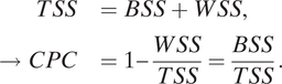(1) $$ \begin{array}{rl}\begin{array}{rl}TSS& =BSS+WSS,\\ {}\to CPC& =1-\frac{WSS}{TSS}=\frac{BSS}{TSS}.\end{array}& \end{array} $$

More formally, the CPC takes the expression in Equation 2, where each individual i in cluster k holds a position on dimension j. Footnote ³ This construction in terms of k and j shows how the CPC facilitates the incorporation of multiple groups and variables, respectively. Expressed in this way, the CPC appears related to a one-way ANOVA F-statistic and the coefficient of determination ( $ {R}^2 $ ). These are useful similarities for deriving properties of the measure (Sections S2.2–S2.5 of the Supplementary Material).

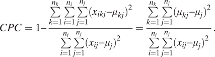(2) $$ \begin{array}{r}CPC=1-\frac{\sum_{k=1}^{n_k}\sum_{i=1}^{n_i}\sum_{j=1}^{n_j}({x}_{ikj}-{\mu}_{kj}{)}^2}{\sum_{i=1}^{n_i}\sum_{j=1}^{n_j}({x}_{ij}-{\mu}_j{)}^2}=\frac{\sum_{k=1}^{n_k}\sum_{j=1}^{n_j}({\mu}_{kj}-{\mu}_j{)}^2}{\sum_{i=1}^{n_i}\sum_{j=1}^{n_j}({x}_{ij}-{\mu}_j{)}^2}.\end{array} $$

Because intra-state political dynamics, the number and nature of sociopolitical cleavages, and the size and number of political coalitions typically vary across countries or within countries over time, one additional modification is needed to make the CPC appropriate for comparison across contexts with varying numbers of observations, variables, and clusters. The expression in Equation 2 will be biased upward in small samples, so I incorporate corrections for lost degrees of freedom and express the adjusted CPC in Equation 3:Footnote ⁴

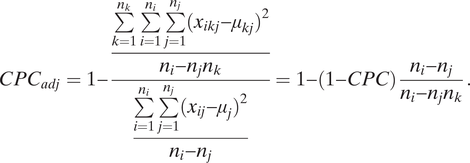(3) $$ \begin{array}{r}CP{C}_{adj}=1-\frac{\frac{\sum_{k=1}^{n_k}\sum_{i=1}^{n_i}\sum_{j=1}^{n_j}({x}_{ikj}-{\mu}_{kj}{)}^2}{n_i-{n}_j{n}_k}}{\frac{\sum_{i=1}^{n_i}\sum_{j=1}^{n_j}({x}_{ij}-{\mu}_j{)}^2}{n_i-{n}_j}}=1-(1-CPC)\frac{n_i-{n}_j}{n_i-{n}_j{n}_k}.\end{array} $$

By explicitly modeling both $ BSS $ and $ WSS $ , the CPC accounts for both features of polarization. It increases when the distance between groups increases or when groups become more tightly concentrated around their collective ideal point, with the rate of those increases depending on the relative levels of $ BSS $ and $ WSS $ .

To illustrate the importance of both features and how the CPC produces more accurate estimates than existing measures, consider the stylized distributions in Figure 1. They imitate four possible combinations of intergroup heterogeneity and intragroup homogeneity. The distribution in plot a has neither feature—two clusters are faintly apparent, but they are close together and display little cohesion. Plot b has high intragroup homogeneity and low intergroup heterogeneity, and plot c has the reverse. The group means are the same in plot b as in plot a, but the groups are more concentrated. Intragroup homogeneity is the same in plot c as in plot a, but group means are further apart. Finally, plot d has high levels of both characteristics.

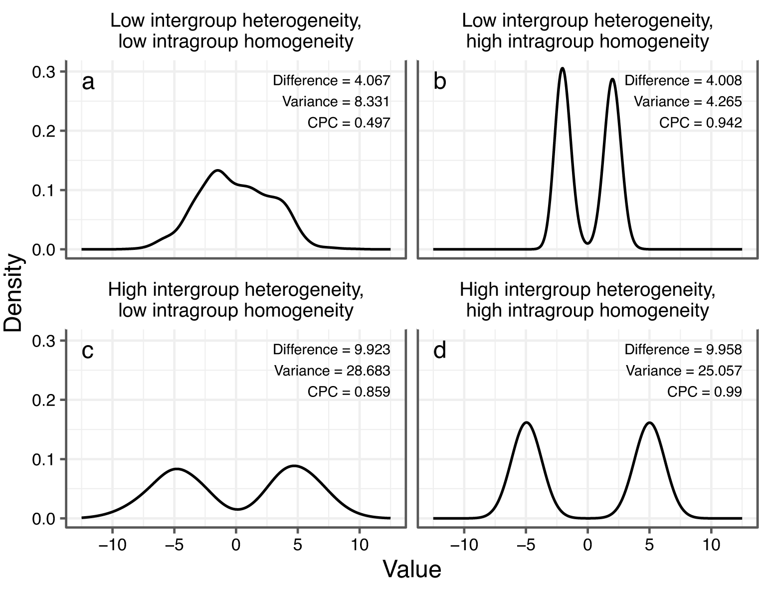
Figure 1.

Stylized Distributions of Polarization Features

Note: Simulated bimodal Gaussian mixture distributions with $ {\mu}_{global}=0 $ . Labels show polarization levels according to each measure. Plots labeled a–d to correspond to explanations in text.

A measure accurately capturing polarization should indicate more polarization in plots b–d of Figure 1 relative to plot a and less polarization in plots a–c relative to plot d. Plot labels display the polarization estimate for each distribution based on difference-in-means, variance, and the CPC. In all cases, higher numbers indicate greater polarization.

Difference-in-means successfully distinguishes between plots a and c and between plots b and d of Figure 1, assigning a higher polarization estimate to the latter plot in each pairing, but it cannot distinguish plot a from b nor plot c from d. It assigns identical polarization estimates to each distribution even though plots b and d are qualitatively more polarized than plots a and c, respectively, reflecting why Levendusky and Pope (Reference Levendusky and Pope2011) urge scholars to “go beyond the mean” when measuring polarization. Variance is frequently offered as one way of doing that, but it performs even worse here. It, too, distinguishes between plots a and c and between plots b and d, but it assigns lower polarization estimates to plots b and d relative to plots a and c, opposite the conceptual understanding of polarization. This simple exercise suggests that the most common measures may allow polarization to go undetected in some cases and, in others, identify it where it does not exist. The CPC is the only measure of the three that accurately captures the qualitative differences between all four distributions.

The Supplementary Material includes several validation exercises (Mehlhaff Reference Mehlhaff2023). Sections S3.1 and S3.2 of the Supplementary Material show that, compared to difference-in-means and variance, the CPC more consistently captures both features of polarization in univariate and bivariate contexts and in distributions with two, three, and four groups. Sections S3.3 and S3.4 of the Supplementary Material show the CPC can be sensitive to outliers and large differences in group size, though it still outperforms existing measures and scaling the input data ameliorates outlier sensitivity. Section S4 of the Supplementary Material benchmarks each measure’s performance against “ground-truth” data gathered from human annotators.

POLARIZATION IN CONGRESS: A MULTIDIMENSIONAL TEST

I investigate the well-established rise in congressional polarization in the United States, showing that the CPC recovers this increase in multidimensional data. I calculate congressional polarization using DW-NOMINATE (Lewis et al. Reference Lewis, Poole, Rosenthal, Boche, Rudkin and Sonnet2021), which uses a scaling procedure to estimate the ideal points of legislators in a two-dimensional latent space. The first dimension is said to capture economic issues and the second racial and other social issues. Because the CPC is expressed in terms of j in Equation 2 and Equation 3, it can incorporate both variables without needing to average over them or create an index.

A steady increase in party polarization has been one of the defining features of congressional politics in the late twentieth and early twenty-first centuries, occurring in economic, racial, and cultural issue domains (Layman and Carsey Reference Layman and Carsey2002). Focusing on the period from 1975 to the present, each measure of polarization should therefore indicate increases whether they examine only the first NOMINATE dimension or incorporate both.

Polarization estimates for each Congress appear in Figure 2. All measures generally capture the expected trend in the first NOMINATE dimension. However, performance diverges with the addition of the second dimension.Footnote ⁵ Difference-in-means detects the increase in polarization that occurred in the House, but it implausibly suggests the Senate didn’t begin polarizing until the mid-2000s and, even in 2019, remained almost a full standard deviation less polarized than it was in the late 1970s. Variance does even worse with the addition of the second dimension, suggesting flat or declining polarization levels leading up to the present-day. The CPC consistently recovers trends that more closely reflect expectations in both one and two dimensions.

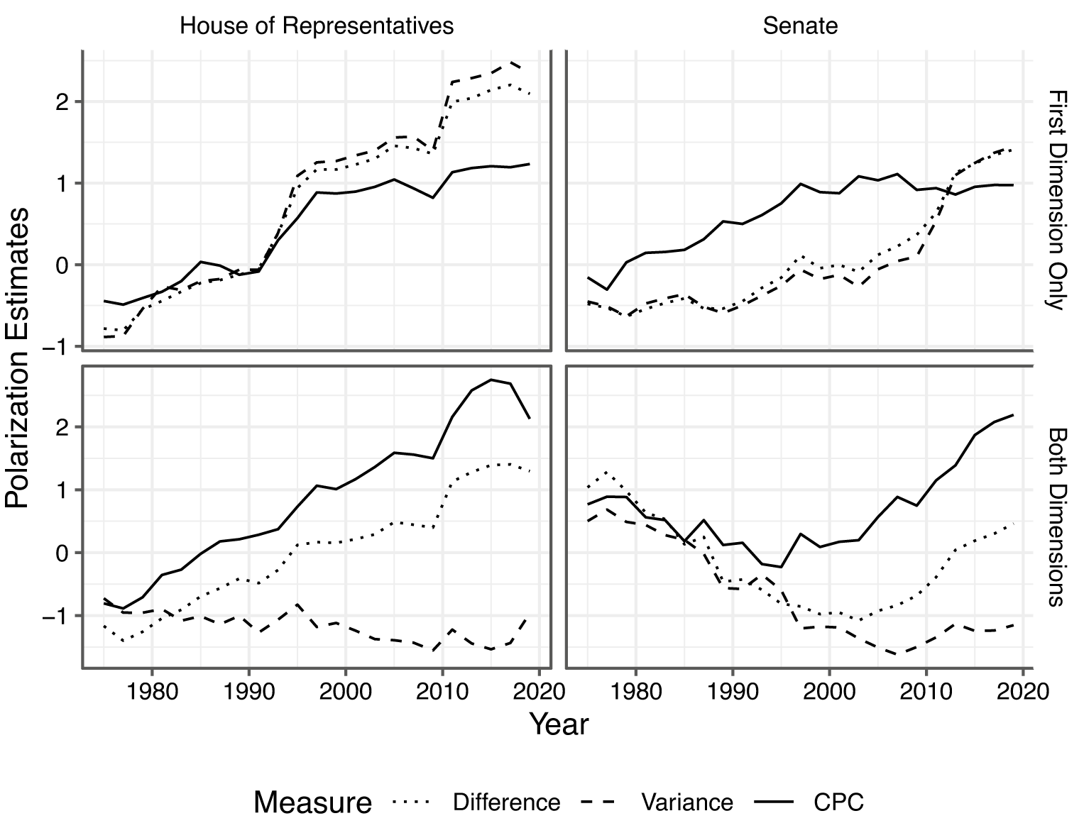
Figure 2.

Congressional Polarization Estimates

Note: Calculated using NOMINATE ideal point estimates; each measure unit-normalized to enable comparison. All point estimates are available in the online replication materials.

Evaluating general trends is informative but, in some cases, it is difficult to tell how much estimates deviate from each other. To assess whether those deviations lead each measure to reflect polarization more or less closely, I evaluate how polarization estimates correlate with each chamber’s party unity score—the percentage of legislators voting with their party on votes in which a majority of Democrats oppose a majority of Republicans (Brookings Institution Reference Jardina and Ollerenshaw2022). Each measure should indicate a positive correlation between polarization and party unity.

Results are shown in Table 1. All three measures correlate highly with party unity when examining only the first dimension, though the CPC holds a narrow performance advantage in the House and a significant one in the Senate. When considering both dimensions, difference-in-means shows a strong correlation in the House, though it is again narrowly bested by the CPC. Variance struggles in both chambers, suggesting negative associations between polarization and party unity. Though correlations with all measures are lower in the Senate, the CPC is the only measure that still shows a positive association with party unity.

Table 1.

Correlation Between Congressional Polarization Estimates and Party Unity Scores

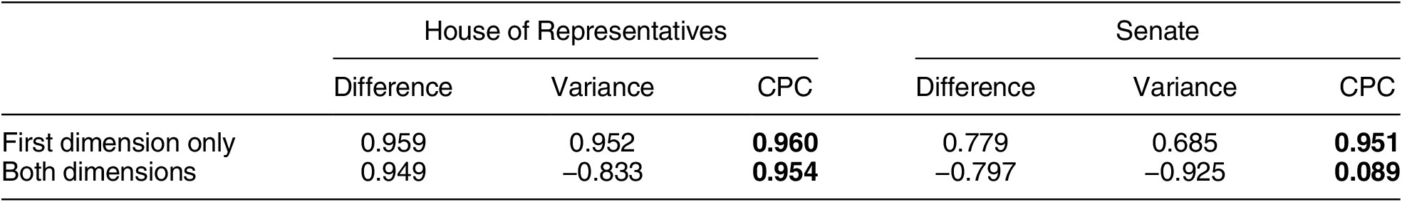
Note: Bolded values denote measure with highest correlation.

This underscores an important benefit of the CPC. Aldrich, Montgomery, and Sparks (Reference Aldrich, Montgomery and Sparks2014) show that high-dimensional estimates are crucial for accurate ideal point estimation, especially in polarized contexts. Researchers using current measures may need to ignore higher-dimensional information as a pragmatic matter, but the CPC allows it to be preserved, resulting in more accurate polarization estimates.

COMPARATIVE ELITE POLARIZATION: A MULTI-GROUP TEST

Measuring polarization in multi-party systems is a persistent challenge (Gidron, Adams, and Horne Reference Gidron, Adams and Horne2020; Wagner Reference Wagner2021). To demonstrate that the CPC can capture polarization across contexts with different numbers of groups, I use a set of elite ideological ideal points from six Western countries (Barberá Reference Barberá2015). As depicted in Figure 3a, these countries differ in the extent to which their latent elite groups are internally homogeneous and externally heterogeneous, and even in how many groups exist within each country. The United Kingdom and Netherlands have high intergroup heterogeneity, the United States has high intragroup homogeneity, and Spain has a fair amount of both. Italy and Germany both have two identifiable modes, but their intragroup homogeneity is relatively low.

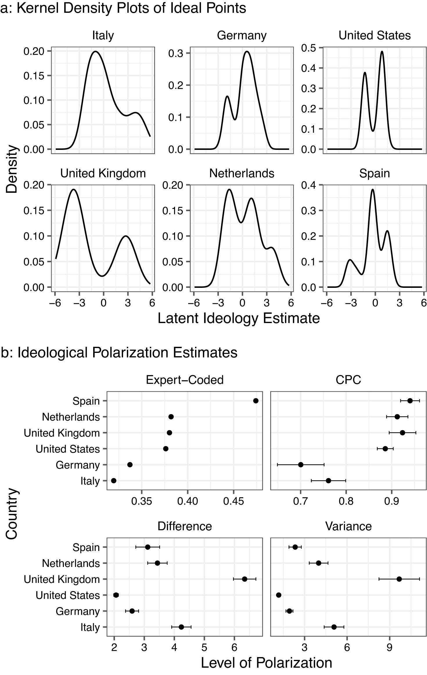
Figure 3.

Estimates of Elite Polarization

Note: Kernel density plots for each country (a) and polarization estimates with bootstrapped 95% confidence intervals (b). The online replication materials present point estimates and standard errors.

With all this variation, it is difficult to identify polarization levels simply by evaluating density plots. To generate expectations for how countries should compare in their levels of elite ideological polarization, I apply Dalton’s (Reference Dalton2008) measure of party system polarization to expert-coded data on left–right party positions (Düpont et al. Reference Düpont, Kavasoglu, Lührmann and Reuter2022). These benchmarks appear in the upper-left facet of Figure 3b and reveal three groupings. Italy and Germany have similar, low levels of polarization. The United States, United Kingdom, and Netherlands are similar to each other in their polarization levels, all higher than those in Italy and Germany. Finally, Spain has by far the highest level of polarization. A well-performing measure of polarization applied to the elite ideology data in Figure 3a should generally reflect these expert judgments.

The other three facets in Figure 3b display the degree to which difference-in-means, variance, and the CPC suggest the party systems are polarized. CPC estimates, shown in the upper-right facet, approximate the expert-coded data much better than difference-in-means or variance do.Footnote ⁶ The CPC indicates that Germany and Italy are the least polarized countries, with the United States, United Kingdom, and Netherlands significantly more so. Though the CPC does not capture the large difference between Spain and the Netherlands that appears in the expert-coded data, it does identify Spain as the most polarized country in the sample.

In contrast, difference-in-means and variance often produce polarization estimates at odds with the expert-coded benchmarks, not to mention the visual representation of the data. Both measures suggest the United States is the least polarized of the six countries, with Italy the second-most polarized despite a near-unimodal distribution of ideal points. Worse still, both difference-in-means and variance suggest polarization in Spain is relatively low, while the expert-coded data show it as by far the highest. In short, they fail to produce polarization estimates that resemble country-expert judgments when there are varying numbers of groups in the data, even in the simplest unidimensional space. The CPC much more closely reflects how experts view ideological polarization in party systems.

AFFECTIVE POLARIZATION: MULTIPLE DIMENSIONS AND GROUPS

In the United States, affective polarization appears to run deeper than ideological or issue polarization (Mason Reference Mason2018), and a robust research program examines this development in comparative perspective (Wagner Reference Wagner2021). In the previous two applications, I addressed problems associated with multidimensional and multi-group data separately. By employing party affect data, I can address them simultaneously. Party systems have different numbers of parties across cases, meaning the number of groups present in the data will vary. The number of parties also determines the number of dimensions; respondents’ assessments across multiple party feeling thermometers represents the several dimensions of their party affect. A measure of polarization should be able to accommodate both sources of variation. To estimate affective polarization, I apply each measure to party feeling thermometers (see also Gidron, Adams, and Horne Reference Gidron, Adams and Horne2020; Ward and Tavits Reference Ward and Tavits2019) from module four of the Comparative Study of Electoral Systems (CSES).

One way to assess validity is to calculate correlations between polarization estimates produced by each measure and indicators that tap attitudes theoretically related to party affect.Footnote ⁷ The CSES contains several good candidates. First, the proportion of respondents indicating “it makes a big difference who is in power.” Second, the proportion who believe “who people vote for can make a big difference.” These statements both capture the degree to which respondents believe their political system presents starkly differentiated options to voters, a belief that likely intensifies with stronger party affect (Ward and Tavits Reference Ward and Tavits2019). Third, the proportion of respondents expressing they “feel very close” to their political party. Respondents should hold their party identity more intensely when their party affect is strong (Mason Reference Mason2018). Finally, the proportion of respondents indicating they occupy extreme positions of a left–right self-placement scale. Citizens tend to distrust parties more when those parties are ideologically distant, so the degree of ideological extremity should also be related to affective polarization (Wagner Reference Wagner2021).Footnote ⁸

Figure 4 illustrates how affective polarization correlates with each of these items. Each variable should exhibit positive correlations with polarization estimates. That is true of CPC estimates in all four cases. Difference-in-means and variance also uncover a strong, positive relationship between affective polarization and ideological extremity, but their relationships with other variables are less consistent. Difference-in-means uncovers positive correlations between polarization and beliefs about whether it matters who is in power, but variance displays negative associations with that correlate as well as beliefs about whether one’s vote makes a difference. More concerning, difference-in-means and variance suggest that polarization is negatively related to respondents feeling “very close” to their party. This result would seem to be at odds with the very definition of affective polarization, part of which emphasizes in-group affection, a sentiment that should strengthen when group members are more similar to each other. This finding lends further credence to the notion that the measures most often used to measure polarization do not successfully capture intragroup homogeneity, rendering the accounts of polarization they provide incomplete.

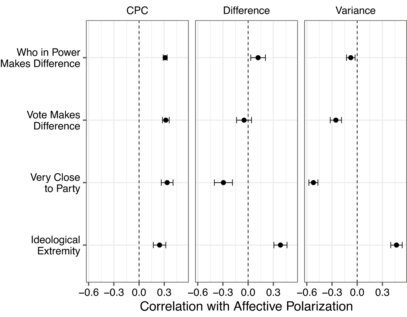
Figure 4.

Correlates of Affective Polarization

Note: Error bars give bootstrapped 95% confidence intervals. Full results reported in online replication materials.