Introduction

Multi-year mean values of ^l8O/¹⁶O relative to standard mean ocean water (SMOW) (δ ¹⁸O, in ‰) determined from samples collected on the Greenland ice sheet are used in climalological and glaciological investigations (e.g. Reference Reeh, Thomsen and ClausenReeh and others, 1987b; Reference Clausen, Gundestrup, Johnsen, Bindschadler and ZwallyClausen and others, 1988; Reference Johnsen, Dansgaard and WhileJohnsen and others, 1989). This study presents stepwise statistical analyses based on δ ¹⁸O reported for 46 sites (Fig. la) as the dependent variable, and four independent variables: latitude (L, in °N); surface elevation (H, in m); multi-year mean surface temperature (T_s, in K) normally determined from 10 m borehole temperature, mean surface temperature in 1979 (T_r, in K) obtained by bilinear interpolation from the Nimbus-7 Temperature Humidity Infrared Radiometer (THIR) database (Reference ComisoComiso, 1994); and multi-year mean shortest distance to the open ocean denoted by the 10% sea-ice concentration boundary (D, in km) obtained from the Nimbus-7 Scanning Multichannel Microwave Radiometer (Reference Gloersen, Campbell, Cavalieri, Comiso, Parkinson and ZwallyGloersen and others, 1992). Use of a different sea-ice concentration boundary to denote open ocean (e.g. 20% open water) docs not introduce significant differences in the statistics. The purpose is to define multivariate models applied to a 100 km grid database (Figure lb) and produce contoured distributions of δ ¹⁸O. These distributions may be used in advection studies (e.g. Reference Johnsen, Dansgaard and WhileJohnsen and others, 1989) or to derive ice-flow adjustments (e.g. Reference Reeh, Hammer, Thomsen and FisherReeh and others, 1987a).

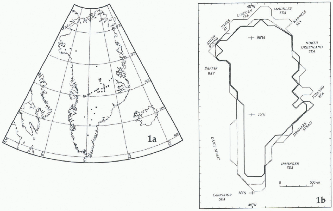
Fig. 1. (a) Greenland, showing the location of the 46 data sites for which δ¹⁸O values have been reported (full squares; some overlap). (b) Schematic map of Greenland. The outer, thin line is roughly coincident with the coastline, enclosing an area represented by 216 gridpoints 100 km apart. The double line is roughly coincident with the boundary of the conterminous ice sheet, an area represented by 187 gridpoints. The inner, thick line is an approximation to the position of the equilibrium line that encloses an area represented by 160 gridpoints (the boundary of the areas is shown in (Figs 2 and 3).

In the following sections, the statistics are significant at the 99.99% confidence Level (F statistic under the null hypothesis showing a probability of P ≤ 0.0001) unless stated otherwise. A confidence level selected for a particular model to determine which variables contribute at that level (or better) to the explanation of variation is a separate statistic from the P-value attained by the model.

Sample Site Database

The initial compilation included data for a total of 62 sites (after the analyses were completed we were informed of a few more sites available for northern Greenland (K. Steffen, personal communication, August 1996)). Data for 46 of the 62 sites were retained for analyses; these are from Reference Müller, Stauffer and SchriberMüller and others (1977), Sehriber and others (1977), Reference Clausen and HammerClausen and Hammer (1988), Reference Clausen, Gundestrup, Johnsen, Bindschadler and ZwallyClausen and others (1988), Reference Johnsen, Dansgaard and WhileJohnsen and others (1989), Reference DansgaardDansgaard and others (1993), Reference Grootes, Stuiver, White, Johnsen and JouzelGrootes and others (1993) and Reference Fischer, Wagenbach, Laternser and HaeberliFischer and others (1995). Most of the data for 18 sites from Reference Fischer, Wagenbach, Laternser and HaeberliFischer and others (1995) were obtained by interpolation. Actual values were obtained after the analyses were completed (H. Fischer, personal communication, August 1996). The differences between the interpolated and actual values are minor. The largest differences are in elevation; differences in latitude and longitude would introduce small changes in D and T_r values. However, use of the actual values would not introduce significant changes in the statistics presented in this study.

Data for 14 sites were excluded from the analyses because the samples were collected in the ablation zone or in areas of widespread summer melt and percolation. These were Warming Land (81.50°N, 52.0°W; Reference Reeh, Thomsen and ClausenReeh and others, 1987b), nine sites in the Thule area centered at approximately 76.5°N, 68°W (Reference Reeh, Thomsen, Frich and ClausenReeh and others, 1990), Paakitsoq (69.75°N, 49.0°W; Reference Reeh, Oerter, Letréguilly, Miller and HubertenReeh and others, 1991), Storstrømmen, (77.40°N, 23.0°W; Reference Reeh, Oerter, Miller and PeltierReeh and others, 1993), and Drill Sites I and II, at approximately 70.00°N, 49.5°W, and 69.92°N, 49.4°W, respectively (Reference Clausen and StaufferClausen and Stauffer, 1988).

The reliability of T_r values interpolated from the THlR database with a resolution of approximately 30 × 30 km (Reference ComisoComiso, 1994) was assessed by a simple regression of the form T = f(T) (N48, where N denotes the number of sites in the set: the coefficient of correlation (R) is 0.966 and the root mean square residual (rms) is 0.81). Data for two sites showed the largest departure (>3 rms): Site V on the North ice cap, 77.07°N, 70.4°W (Reference Müller, Stauffer and SchriberMüller and others, 1977: Reference Schriber, Stauffer and MüllerSchriber and others, 1977), and a site on the Renland ice cap, (71.25°N. 27.5°W; Reference JohnsenJohnsen and others, 1992; Reference HanssonHansson, 1994). Data for these sites were excluded from the analyses discussed below.

The descriptive statistics for the N46 set (see Table 1) show that the mean of T_r is practically the same as that of T ^s, although the standard deviation and range of T_r values are much smaller. Nevertheless, the correlation matrix (Table 2) shows that where there is strong correlation between T_s and other variables (δ¹⁸O, H), these remain strong when T_r is substituted. The stepwise analysis of δ¹⁸O = f(L, H, T_s, D) at the 99.9% confidence level shows that T _s is the only variable to enter the model in the forward mode or remain in the model in the backward mode (Table 3), defining a robust bivariate model (R is 0.986, rms is 0.55):

(1)

Table 1. Descriptive statistics

Table 2. Correlation matrices

Table 3. Summary of stepwise regression analyses (N46,δ¹⁸O as the dependent variable)

The same result is obtained from runs in the forward mode at the 95% and 90%, confidence levels. However, the result from runs at these confidence levels in the backward † Best model. Same results as a run in the backward mode at the 90% confidence level. mode is different: L, T _s and D remain in the model, and H is removed. This stepwise model is equally robust (R is 0.987, rms is 0.53):

(2)

The practically equal R and rms values for Equations (1) and (2) indicate that both models provide the same reliability. Nevertheless, the inclusion of L and D in Equation (2) enhances model sensitivity to predict δ¹⁸O; this is substantiated by the results of inversions of Equations (1) and (2) using gridpoint data, described below.

Gridpoint Database

The gridpoint locations were determined from a pattern with origin lines at 135°W −45°E, and 45°W. The 160 locations that lie in the area of net accumulation at the surface were selected on the basis of an assumed north to south linear variation of the elevation of the equilibrium line (Reference Giovinetto and ZwallyGiovinetto and Zwally, 1996). The variation was not adjusted for differences between north and south facing slopes (e.g. Reference BensonBenson, 1962), or between eastern and western flanks at particular latitudes (e,g. Reference ReehReeh, 1985) because it does not affect the findings of our study.

The gridpoint data (N160) on latitude (L_i , in °N), surface elevation (H_i, in m.), and mean annual surface temperature (T _si in K) were obtained by visual interpolation from the surface contour and isotherm maps of Reference OhmuraOhmura (1987). The T _ri and D_i data were obtained as described for T_r and D in the sample site database.The descriptive statistics for the N160 set are listed in Table 1.

The gridpoint database was compiled before the publication of a more recent topographic map. We compared H_i and surface elevation values obtained (i) by visual interpolation from the latest surface contours map (Reference WeidickWeidick, 1995), and (ii) by bilinear interpolation from the ERS-1 radar-altimeter data. The comparisons are based on data for 168 grid-point locations that include about 130 of the 160 used in this study. We obtained R values between 0.951 and 0.953. The difference in elevation values obtained from each surface Contour map is due, in part, to the overlay of a fixed-grid pattern over maps of different projections and with different standard lines. The differences between these and the elevation values obtained from the ERS-1 database is due, in part, to round off (to 0.1°) L_i and longitude values entered in the gridpoint database. This implies an error in location of several km north to south and in most areas of at least 1 km east to west, whereas the ERS-1 data resolution is of about 500 m (Reference WeidickWingham, 1995). Therefore, we did not update the H_i data.

Areal Distribution of δ¹⁸O

The inversions of Equation (1) using the N160 database and either T _si or T _ri (i.e. (δ¹⁸O)_bs = f(T _si), and (δ¹⁸O)_br. = f(T _ri)) result in mean, maximum and minimum values that are remarkably close to those obtained by the inversions of Equation (2) (i.e. (δ¹⁸O)_ms = f(L_i, T _si, D _i), and (δ¹⁸O)_mr = f(L_i, T _ri, D _i) (Table 4). The correlation matrix for the N160 set (Table 2) lists the strong correlations that would be expected from Equations (1) and (2) between the derived terms (δ¹⁸O)_ms, (δ¹⁸O)_mr and the input terms T _si and T _ri (R values of 0.996 and 0.994). The covariation between H_i and the temperature terms (R values of 0.633 and 0.672) is weak relative to the strong covariation noted for the sample sites data (Table 2, N46: R values of 0.873 and 0.986). This decay is also noted in the relationship between δ¹⁸O and elevation (R is 0.872 for the sample site data, and R values are 0.684 and 0.727 for the gridpoint data).

Table 4. Descriptive slalistics edicled

The distributions of (δ¹⁸O)_bs and (δ¹⁸O)^br as well as of (δ¹⁸O)_ms and (δ¹⁸O)_mr (Figs 2a, b and 3a, b, respectively) show that, in general, the isopleths are oriented perpendicular to flow lines (e.g. Reference Radok, Barry, Jenssen, Keen, Kiladis and McInnesRadok and others, 1982), thus facilitating any derivation of adjustments for δ¹⁸O series obtained from deep cores.

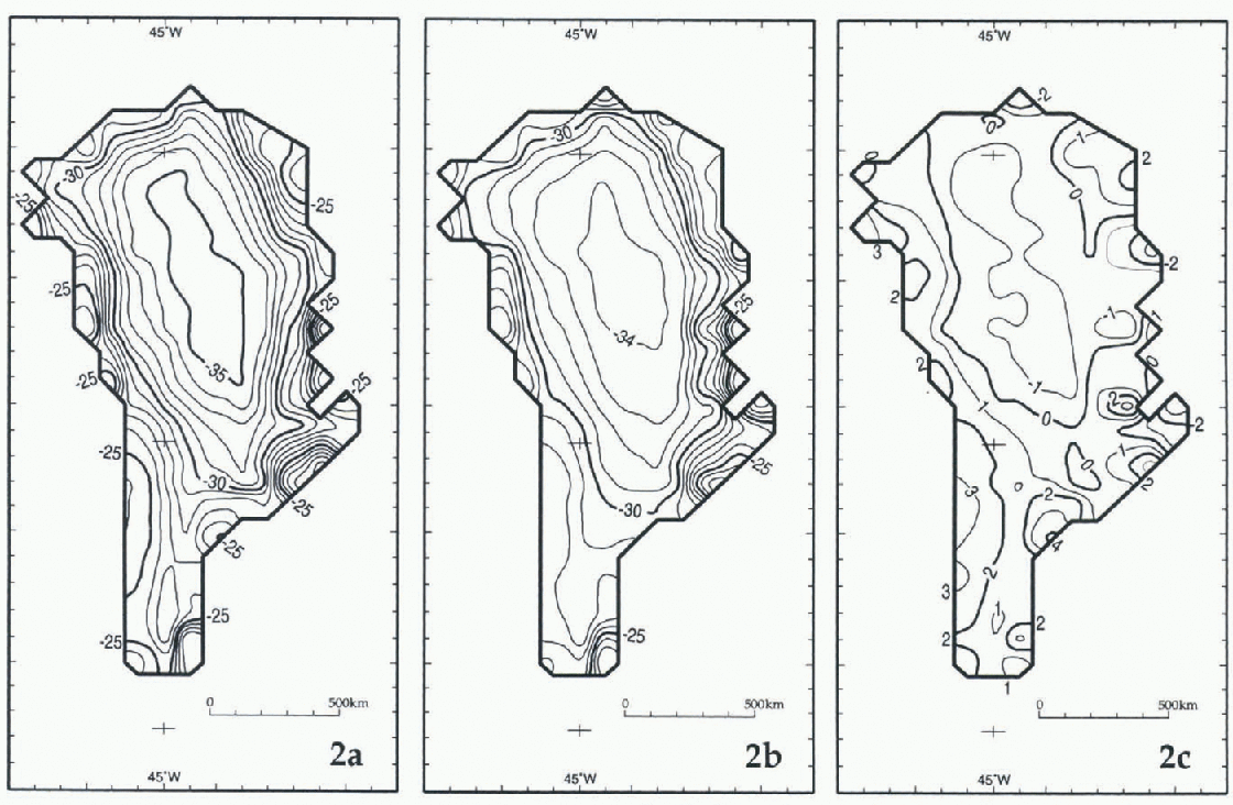
Fig. 2. The area of Greenland delimited by the equilibrium line, (a) Distribution of (δ¹⁸O)_bs = f(T _si). (b) Distribution of (δ¹⁸O)_br = f(T _ri). (c) Distribution of Δ_b = (δ¹⁸O)_bs - (δ¹⁸O)_br.

Fig. 3. The area of Greenland delimited by the equilibrium line. (a) Distribution of (δ¹⁸O)_ms. (b) Distribution of (δ¹⁸O)_mr. (c) Distribution of Δ_m - (δ¹⁸O)_ms - (δ¹⁸O)_mr.

We evaluate first the difference between bivariate models using either T _si or T _ri data (i.e. Δ _b = [(δ¹⁸O)_bs-(δ¹⁸O)_br] (Fig. 2c). The distribution of Δ _b indicates differences of −1‰ in the north-central region, changing to + l‰ in the south-central region. In these regions lie most of the length of the main drainage divides, where flow lines originate. In general, Δ _b becomes larger toward the equilibrium line, except in four regions where it decreases to zero: these are the sectors of the Smith Sound-Nares Strait, McKinley Sea, southern North Greenland Sea-northern Iceland Sea, and southern Denmark Strait. Otherwise, Δ _b remains positive in the southern outlying slopes, i.e. toward the equilibrium line in the sectors of the Davis Strait (+3‰), Labrador Sea (+2‰) and Irminger Sea (+4‰). It also † Δ_b = [(δ¹⁸O)_bs - (δ¹⁸O)_br]: Δ_m = [(δ¹⁸O)_ms - (δ¹⁸O)_mr]: Δ_r = [(δ¹⁸O)_br - (δ¹⁸O)_mr]. becomes larger toward the equilibrium line, but the increases are signed in a complex pattern in the sectors of the Denmark Strait-Iceland Sea (+3‰, decreasing northward to −3‰), and around the northern outlying slopes in the sectors of Baffin Bay (+2‰), the Lincoln and western McKinley Seas (−2‰>), the Wandels Sea (+1‰), and the North Greenland Sea (from +2‰ in the central part of the sector, to −3‰ in the southern part).

Due to the dominance of the temperature term in both Equations (1) and (2), the difference between multivariate models using either T _si or T _ri data (i.e. Δ_m[(δ¹⁸O)_ms — (δ¹⁸O)_mr], is practically identical (Figure 3c). This similarly is also noted in the descriptive statistics, which show insignificant differences between Δ_b and Δ_m (Table 4).

We evaluate next the difference introduced by the multivariate models that include the effects of latitude and distance to the open ocean, for this, we select the models that include T_r data, and produce a contoured distribution of Δ_r = (δ¹⁸O)_br - (δ¹⁸O)_mr (Fig. 4, Table 4). The difference in distribution introduced by the multivariate model is small (mean −0.22‰, std dev. 0.03). The larger ‰_r values are noted in the northwest region of the ice sheet (between −0.50‰ and −1.15‰), decreasing to zero in a broad zone extending from the sector of Baffin Bay to the Irminger Sea sector. Values of Δ_r increase toward the southern region of the ice sheet (between +0.10‰ and +0.35‰).

Fig. 4. The area of Greenland delimited by the equilibrium line. Distribution of Δ_r = (δ¹⁸O)_br - (δ¹⁸O)_mr.

Discussion and Conclusions

At present, given the relatively small number and sporadic areal distribution of firn-temperature measurements at depths > 10 m, and the paucity of meteorological records from the interior (manned as well as automatic weather stations), we believe that the distribution of (δ¹⁸O)_ms (Fig. 3b) is the more reliable pattern. The reliability of this pattern, as well as that produced using (δ¹⁸O)_ms (Fig. 2b) may be improved if δ¹⁸O values for the sample sites could be adjusted to represent only the last 10–20 years of records available at each site (some of the δ¹⁸O values entered in the database are from samples spanning at least a few centuries).

The distribution of (δ¹⁸O)_mr is produced from the inversion of a robust multivariate model that includes Nimbus-7 THIR mean annual temperature data, latitude and mean annual shortest distance to the open ocean (R is 0.987, rms is 0.53). It shows large differences relative to the distribution produced using a bivariate model based on temperature values interpolated from surface data (Δ_m = 0.34 ± 0.12‰, with a range of −3.43‰ to +4.41‰). The larger differences show in the outer slopes, i.e. the zone characterized by steep surface gradient close to the equilibrium line. These are the areas where interpolation of surface-temperature data would be least reliable. Nevertheless, in more than half the accumulation area of the ice sheet, in the interior where the main drainage divides lie, the difference is −1‰ in the north and central part, and + 1‰ in the southern part.

The distribution of (δ¹⁸O)_mr) also shows differences from a distribution based on a bivariate model using only Nimbus-7 THIR data. The inclusion of latitude and distance to the open ocean induces differences (Δ_r = 0.22 ± 0.02‰, with a range of −1.18 to 0.40‰) that are smaller than the error of prediction in more than three-quarters the accumulation area of the ice sheet. The only differences larger than the error are found in the northwest region of the ice sheet.