






Introduction
Sea ice is a fundamental feature in the Arctic climate system that enhances the albedo of the ocean surface and forms a physical barrier that inhibits ocean-atmosphere heat, moisture and momentum fluxes (Juricke and Jung, Reference Juricke and Jung2014; Vihma, Reference Vihma2014). The loss of sea ice is a key factor in the accelerated warming of the Arctic (Serreze and others, Reference Serreze, Barrett, Stroeve, Kindig and Holland2009), where temperatures are increasing at a rate twice the global average (Blunden and Arndt, Reference Blunden and Arndt2015). A variety of socioeconomic interests are also tied to the presence or absence of sea ice, increasing the demand for more skillful predictions of the evolving ice coverage. However, seasonal ice forecasts remain challenging due in part to a high degree of interannual variability (Francis and Hunter, Reference Francis and Hunter2006) stemming from a complex, and not fully resolved, system of dynamic (Zhang and others, Reference Zhang, Lindsay, Steele and Schweiger2008) and thermodynamic (Stroeve and others, Reference Stroeve, Holland, Meier, Scambos and Serreze2007; Mills and Walsh, Reference Mills and Walsh2014) processes.
Large-scale atmospheric circulation patterns, in combination with ocean currents, drive sea-ice advection and export, thereby dynamically impacting seasonal sea-ice coverage (Parkinson and Comiso, Reference Parkinson and Comiso2013; Tilling and others, Reference Tilling, Ridout, Shepherd and Wingham2015). Thermodynamic processes, meanwhile, regulate the freezing and melting cycles. The surface radiative budget in particular is critical to determine the timing and magnitude of the seasonal melt at the ice–ocean and ice–atmosphere boundaries. Clouds add considerable complexity to the Arctic surface radiative budget (Kay and Gettelman, Reference Kay and Gettelman2009), constituting a mean fractional sky coverage >80% (Liu and others, Reference Liu, Ackerman, Maddux, Key and Frey2010), making realistic representations of ice–atmosphere interactions challenging, though critical. Clouds can impart two competing effects in the radiative budget of the surface: cooling via reflecting incoming solar radiation and warming by emitting downwelling longwave radiation to the surface (Shupe and Intrieri, Reference Shupe and Intrieri2004). The relative magnitude of these effects is variable over sea-ice surfaces with potentially high and seasonally-varying albedo. The impact of Arctic clouds on surface-atmosphere moisture and energy exchanges is also amplified by aridity in this region (Cox and others, Reference Cox, Walden, Rowe and Shupe2015). The net impact of cloud presence in the Arctic varies considerably through the year due to large seasonal oscillations in incident solar radiation and episodic changes to fractional cloud coverage and composition.
Here, we focus on the radiative fluxes commonly associated with variable cloud coverage and composition to better constrain the role of Arctic clouds in seasonal sea-ice declines. Several studies have highlighted how the presence and composition of Arctic clouds, and their related impact on surface radiative fluxes, affect sea-ice concentration and extent (Kay and Gettelman, Reference Kay and Gettelman2009; Barton and Veron, Reference Barton and Veron2012; Choi and others, Reference Choi2014; Liu and Key, Reference Liu and Key2014). Recent study has also found that springtime and early summer radiative fluxes, particularly downwelling longwave fluxes, can regulate the timing of snowmelt onset over sea ice (Maksimovich and Vihma, Reference Maksimovich and Vihma2012) and can initiate processes that affect summer and fall sea-ice extent (Kapsch and others, Reference Kapsch, Graversen and Tjernström2013, Reference Kapsch, Graversen, Economou and Tjernström2014; Cox and others, Reference Cox2016; Kapsch and others, Reference Kapsch, Graversen, Tjernström and Bintanja2016). Other recent study found that decadal-scale variability in summertime conditions outside the Arctic, particularly Pacific sea surface temperatures (Bonan and Blanchard-Wrigglesworth, Reference Bonan and Blanchard-Wrigglesworth2020), can impact September sea-ice conditions by creating Arctic atmospheric conditions favorable to sea-ice melt (Baxter and others, Reference Baxter2019; Ding and others, Reference Ding2019). Huang and others (Reference Huang2019) showed that significant increasing trends in cloud fraction and cloud water path are most widespread in March and April, enhancing downwelling longwave radiation and near surface warming. Even under clear sky conditions, Liu and Schweiger (Reference Liu and Schweiger2017) showed that enhanced downwelling longwave radiation from warm air advection can initiate melt onset in the Beaufort and Chukchi Seas.
In addition to reductions in sea-ice extent and concentration, Arctic sea ice is thinning, resulting in less multi-year sea ice (Kwok, Reference Kwok2018). Surface radiative imbalances, such as those in the spring during periods of melt onset as discussed above, have been shown to impact sea-ice thickness for months after the initial radiative forcing (Letterly and others, Reference Letterly, Key and Liu2016). Thus, here we focus on seasonal ice volume loss, combining both sea-ice concentration and thickness terms. Using satellite observations of ice volume and radiative fluxes, this study seeks to develop an empirical predictive model of seasonal ice volume loss by identifying when volume changes are most sensitive to specific radiative fluxes. In addition to a statistical analysis, we trace the physical mechanisms responsible for converting the radiative forcing into seasonal ice volume loss. A better understanding of the causes of interannual variability in sea-ice melt can inform improvements to both modeling of the Arctic sea-ice cover and to empirical seasonal forecasts.
Data
Cloud radiative flux data
The NASA Langley Research Center distributes monthly Arctic cloud radiative fluxes from the Cloud and Earth's Radiant Energy System (CERES) MODerate resolution Imaging Spectroradiometer (MODIS) Energy Balanced and Filled (EBAF) Surface Product, edition 4.0 (Wielicki and others, Reference Wielicki1996; Kato and others, Reference Kato2018), on a 1° × 1° grid. Specific CERES-EBAF variables used in this study are listed in Table 1. They include downwelling shortwave and longwave radiation (SWd and LWd), net shortwave and longwave cloud radiative effects (CRESW and CRELW), downwelling shortwave and longwave cloud radiative effects (CRE$_{\rm SW_{\rm d}}$ and CRE$_{\rm LW_{\rm d}}$
 ) and the net surface cloud radiative effect (CRENet). The intra-annual variation of some of the key variables is shown in Figure 1. Uncertainties in the monthly gridded product are described in detail by Kato and others (Reference Kato2018), who found an average uncertainty, or mean monthly RMS difference between the gridded Ed4 EBAF surface irradiance product and four Arctic observational stations, of 12 W m−2 (longwave) and 14 W m−2 (shortwave). Three of the four Arctic stations are land-based, however, and irradiances within a 1° × 1° gridcell can be highly variable, making validation in this region challenging.
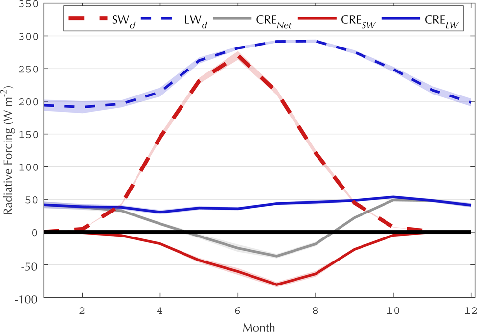
Fig. 1. Arctic (70–90° N) mean monthly radiative fluxes from the CERES-EBAF surface product calculated over the 2000–2017 period, including downwelling longwave (dashed blue), downwelling shortwave (dashed red), longwave cloud radiative effect (solid blue), shortwave cloud radiative effect (solid red) and net cloud radiative effect (solid gray). Shaded contours denote ± 1 SD.
Table 1. CERES-EBAF surface products used in this study
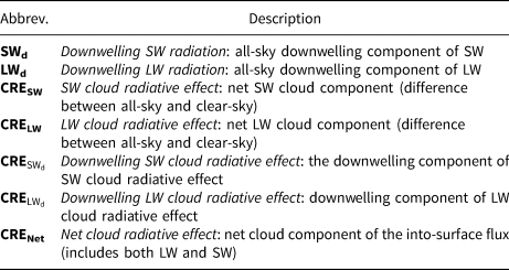
Cloud radiative effect (‘CRE’) describes the difference between the all-sky and clear-sky into-surface flux. The abbreviations ‘LW’ and ‘SW’ refer to longwave and shortwave radiation, respectively.
Sea-ice data
We use two satellite data products along with output from a coupled ice–ocean model to track monthly and interannual changes in Arctic sea-ice volume. Quasi-monthly sea-ice thickness estimates for 2004–2007 are derived from ICESat laser altimetry data. The gridded sea-ice thickness product on a 25 km × 25 km equal-area grid, obtained from the NASA Jet Propulsion Laboratory online portal, represents a composite of data collected during ~35-day observational campaigns in the spring and fall (Kwok and others, Reference Kwok2009). The data domain, here referenced as ‘IS/JPL’, extends over the central Arctic Ocean and serves as the analysis domain in this study, as it is the smallest of all dataset domains (Fig. 2). The mean ICESat-derived sea-ice thickness uncertainty, averaged over all campaigns and the full ICESat domain, is ~ ±0.25 m (±0.28 in spring and ±0.21 in fall), due to snow depth and ice density assumptions made when deriving ice thickness values from laser altimetry measurements (Zygmuntowska and others, Reference Zygmuntowska, Rampal, Ivanova and Smedsrud2014). We obtained CryoSat-2-based ice thickness estimates from the Alfred Wegener Institute for Polar and Marine Research (Hendricks and others, Reference Hendricks, Ricker and Helm2016) for the 2011–2017 period. These data are available on a 25 km × 25 km EASE grid as monthly averages, except for May–September, due to widespread formation of melt ponds and the reduced reliability of satellite freeboard retrievals. Sea-ice thickness estimates from the AWI CryoSat-2 product, hereafter denoted ‘CS-2’, have been found to closely agree with upward looking sonar mooring data and Operation IceBridge retrievals (Sallila and others, Reference Sallila, Farrell, McCurry and Rinne2019) and are similar to other existing CryoSat-2 products, such as the one from Centre for Polar Observation and Modeling (CPOM) (Tilling and others, Reference Tilling, Ridout and Shepherd2018). Uncertainties in both satellite-derived sea-ice thickness datasets are due to noise in the return echoes, variability in the local sea surface and snow signal interference. Gridcell-level uncertainty varies across the domain as a function of data point density. Within the IS/JPL domain, high data point density reduces the uncertainty compared to the peripheral sea-ice regions (Hendricks and others, Reference Hendricks, Ricker and Helm2016), and radar-derived ice thickness uncertainties are comparable to the ICESat thickness uncertainty of ±0.25 m. CS-2 data are trimmed and bilinearly interpolated onto the IS/JPL grid of 25 km × 25 km equal-area cells. The so-called pole hole, where CS-2 data are missing north of 88° N due to the satellite's orbital inclination, is filled by solving a series of elliptical partial differential equations. Valid surrounding pixels provide boundary values to the PDE, resulting in a smoothed surface with thicknesses that tend toward the mean of the surrounding pixels (D'Errico, Reference D'Errico2020). We use the native sea-ice concentration data associated with each source (NSIDC Near-Real-Time DMSP SSMI/S Daily Polar Gridded Sea Ice Concentration for ICESat and EUMETSAT's Ocean and Sea Ice Satellite Application Facility (OSI-SAF) for AWI's CS-2 sea-ice concentration) to compute gridcell ice volume, as described in the ‘Methods’ Section.
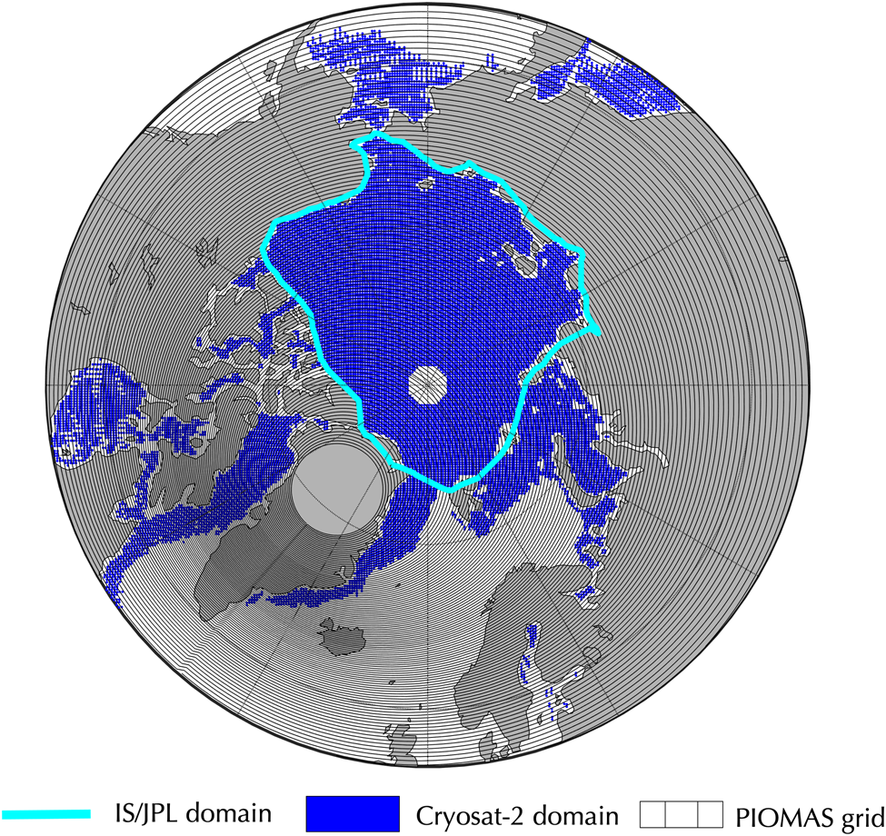
Fig. 2. Boundaries and/or coverage of sea-ice datasets included in this study, with the CS-2 domain shown in blue, and the native curvilinear PIOMAS grid in gray. The IS/JPL domain, outlined in teal, is used as the common analysis domain.
We also utilize continuous monthly modeled sea-ice thickness and concentration fields from the Pan-Arctic Ice–Ocean Modeling and Assimilation System (PIOMAS) (Zhang and Rothrock, Reference Zhang and Rothrock2003). PIOMAS combines the Parallel Ocean Program (POP) model with the Thickness and Enthalpy Distribution (TED) sea-ice model (Zhang and Rothrock, Reference Zhang and Rothrock2003) to produce a variety of continuous ice variables available throughout the study period at monthly resolution. PIOMAS outputs are generated on a generalized orthogonal curvilinear grid, with a mean horizontal resolution of 22 km. PIOMAS is driven by daily mean NCEP/NCAR reanalysis atmospheric variables, and assimilates near-real time observed sea-ice concentration (Anderson and others, Reference Anderson, Bliss and Drobot2014; Tschudi and others, Reference Tschudi, Fowler, Maslanik, Stewart and Meier2016). Since monthly observations of sea-ice volume across the Arctic are not available during summer months, these are estimated from PIOMAS.
Melt onset data over the 2000–2017 period are taken from the SMMR SSM/I brightness temperature product, version 4 (Anderson and others, Reference Anderson, Bliss and Drobot2014; Bliss and Anderson, Reference Bliss and Anderson2018), and used to analyze relationships with cloud radiative properties. Melt onset is defined as the day of year on which melting of the overlying snow on the sea-ice surface is first detected within each gridcell, with values ranging from day 60 to day 244 (Bliss and Anderson, Reference Bliss and Anderson2018).
Methods
Calculation of seasonal sea-ice volume loss
Sea-ice volume is calculated as the product of ice thickness and areal coverage of ice in each 25 km equal-area gridcell. Following the conventions of Laxon and others (Reference Laxon, Peacock and Smith2003, Reference Laxon2013), gridcells with <15% sea-ice concentration, a threshold commonly used to define the sea-ice extent edge (Ogi and Wallace, Reference Ogi and Wallace2007; Serreze and others, Reference Serreze, Barrett, Stroeve, Kindig and Holland2009; Stroeve and others, Reference Stroeve2012; Wang and others, Reference Wang, Chen and Kumar2013; Meier and others, Reference Meier2014; Tilling and others, Reference Tilling, Ridout, Shepherd and Wingham2015), are excluded from the total regional ice volume estimates. Thus, the total sea-ice volume for the study domain is:

where the summation is taken over gridcells with at least 15% sea-ice concentration.
Uncertainties associated with sea-ice thickness and sea-ice concentration observations introduce uncertainty into sea-ice volume calculations. Following Kwok and others (Reference Kwok2009) and assuming an optimal scenario of uncorrelated errors, uncertainty (σT) is estimated by:

where N is the number of gridcells in the domain, h is the mean sea-ice thickness, and A c is the mean gridcell area covered by ice. The absolute sea-ice thickness uncertainty, σh, is conservatively estimated to be ~0.5 m. We use a sea-ice concentration uncertainty of ± 10%, based on NSIDC's algorithm descriptions (http://nsidc.org/data/amsre/data-quality/data-uncertainty.html) which estimate uncertainty to vary from 5% during the winter months to $15\%$ in the wetter summer months. For each 25 km× 25 km gridcell, this implies $\sigma _{A_{\rm c}} = 62.5\, {\rm km}^2$
 . There are approximately N = 11 000 gridcells in the domain, but the number of gridcells entering the estimate can vary slightly during the fall months, when not all gridcells within the domain contain sea ice. The ice volume uncertainty using this approach is < 40 km3 for all months with ICESat or CS-2 data. Additional uncertainties due to the interpolation of missing CS-2 data are estimated to be <± 3 km3, based on the standard error of the surrounding gridcells that fall within a 1° radius of the pole hole.
This study defines the Arctic melt season as the period from 15th March to 15th October, with seasonal sea-ice volume loss defined as the difference in sea-ice volume between these two dates. Monthly averages are assumed to be representative of the 15th of that month. Unfortunately, ICESat data were not consistently collected on the same dates. Therefore, small adjustments are necessary to maintain temporal consistency. For this purpose, we calculate average daily rates of ice volume change for the February–March, March–April and October–November periods from the CS-2 record. These daily rates are then used to correct for the temporal offset in the ICESat record. For example, the midpoint date of the Spring 2004 ICESat campaign is 5th March, 10 days before the desired midpoint date of 15th March. The temporal correction of 10 times the daily February–March volume change rate from CS-2 is then applied to the volume estimates. We use the SD of the daily rates to calculate an uncertainty associated with each temporal adjustment, and compound this with the existing volume uncertainty for ICESat-derived observations, increasing the total uncertainty of ICESat volume estimates to ~200 km3, on average. The resulting monthly ice volume estimates are shown in Figure 3.
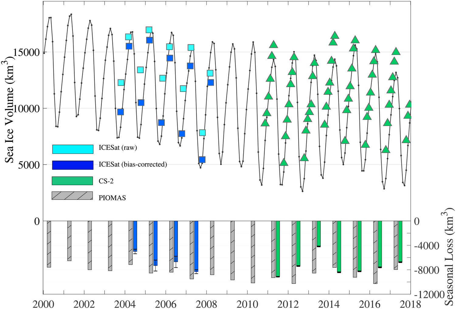
Fig. 3. Top panel: Monthly total sea-ice volume estimates from PIOMAS (black line), raw (light blue) and bias-corrected ICESat (dark blue), and CS-2 (green triangles) from 2000 to 2017. Bottom panel: Net seasonal volume loss (March–October sea-ice volume) for PIOMAS (gray-hatched), ICESat (blue) and CS-2 (green). Uncertainties (±1 − σ) in the total volume loss for observational years are shown, and appear as a dark band in CS-2 years due to the relatively small error.
Linear regression analysis
Linear regression is used to test for a simple linear predictive relationship between any of the radiative variables (Table 1) and the magnitude of regional seasonal ice volume loss. Monthly and bimonthly averages of shortwave and longwave downwelling, cloud-induced downwelling, and the net cloud-induced surface radiative budget, averaged over $70\hbox {--}90^{\circ }$ N (encompassing the central Arctic basin), are used as potential predictors. Prior to areal averaging, predictor radiative variables from CERES, which cover the months from March through July, are resampled from the native 1° × 1° grid to an equally-spaced grid corresponding to the sea-ice data grid. Values over land surfaces are excluded. Total seasonal sea-ice volume loss from years with observational data serves as the dependent variable. R 2, the p-value and the residual are used to evaluate the regression models. The regression is performed initially over all 11 years with ICESat and CS-2 observational data. To check robustness, the regression is then repeated for the first 9 years only, retaining two years (2016 and 2017) for validation.
Results
Sea-ice volume loss
Our calculated spring and fall sea-ice volumes are consistent with existing estimates (Kwok and others, Reference Kwok2009; Laxon and others, Reference Laxon2013; Zygmuntowska and others, Reference Zygmuntowska, Rampal, Ivanova and Smedsrud2014) prior to our applied temporal adjustments. Comparisons of seasonal ice volume loss estimates from PIOMAS, ICESat and CS-2 are shown in Figure 3. The model time series is in reasonable agreement with the observations, with generally larger differences in the early years with ICESat estimates. PIOMAS tends to show lower October and higher March ice volumes, resulting in larger seasonal ice volume loss estimates than are observed by ICESat. Validations performed by Schweiger and others (Reference Schweiger2011) show that PIOMAS modeled ice thicknesses are biased low compared to in-situ data, which contribute to a volume bias of ~10% of the total modeled volume in March and October, as compared to available submarine thickness data. However, PIOMAS run with sufficient observational and reanalysis data, as in this study, performs generally well in capturing the observed seasonality and overall spatial variability of ice thickness across the IS/JPL domain. On this domain, modeled monthly sea-ice volume estimates are valuable for assessing the relative magnitude of monthly changes over the study period, particularly in summer months lacking observations. Previous studies also find potential biases in the observational products, and results from Wang and others (Reference Wang, Key, Kwok and Zhang2016) suggest that ICESat sea-ice thickness retrievals are biased high, particularly in the fall, leading to underestimated seasonal ice volume losses. PIOMAS also predicts greater volume loss than that observed by CS-2 in all years except for 2014. Assuming a consistent bias in PIOMAS over the entire study period, we correct the bias in ICESat ice thickness estimates by setting the average PIOMAS−ICESat bias equal to the average PIOMAS−CS-2 bias in that month (March or October). The temporally-corrected ICESat retrievals in March show an approximate mean bias in ice thickness of + 0.2 m (relative to PIOMAS−CS-2 differences), while those in October show an average bias of +0.4 m. These corrections to ICESat springtime and fall thicknesses result in increases in the estimates of seasonal ice volume losses of, on average, 850 km3 (Fig. 3). The mean seasonal volume loss calculated from both observational datasets is 7190 ±1490 km3, which includes the bias-corrected ICESat average of 6840 km3 and CS-2 average of 7390 km3.
Regression models
The statistically significant (p-value < 0.1) univariate linear regression models relating observed sea-ice loss to radiative flux variables are listed in Table 2, along with several statistical metrics. We find the strongest relationship between seasonal volume loss and March LWd, with an R 2 of 0.49 (p = 0.02). The second most highly correlated individual predictor is CRE$_{\rm LW_{\rm d}}$ averaged over June and July (R 2 = 0.34, p = 0.06). Combined in a multiple linear regression model, March LWd and June–July CRE$_{\rm LW_{\rm d}}$
 together reasonably predict seasonal ice volume losses, with an R 2 of 0.71 (p = 0.007). Over the 11 years, the RMSE of the bivariate regression model is 880 km3, which is ~60% of the RMSE using the 11-year mean as prediction (1490 km3) and 12% of the mean seasonal volume loss. The model's performance is shown graphically in Figure 4.
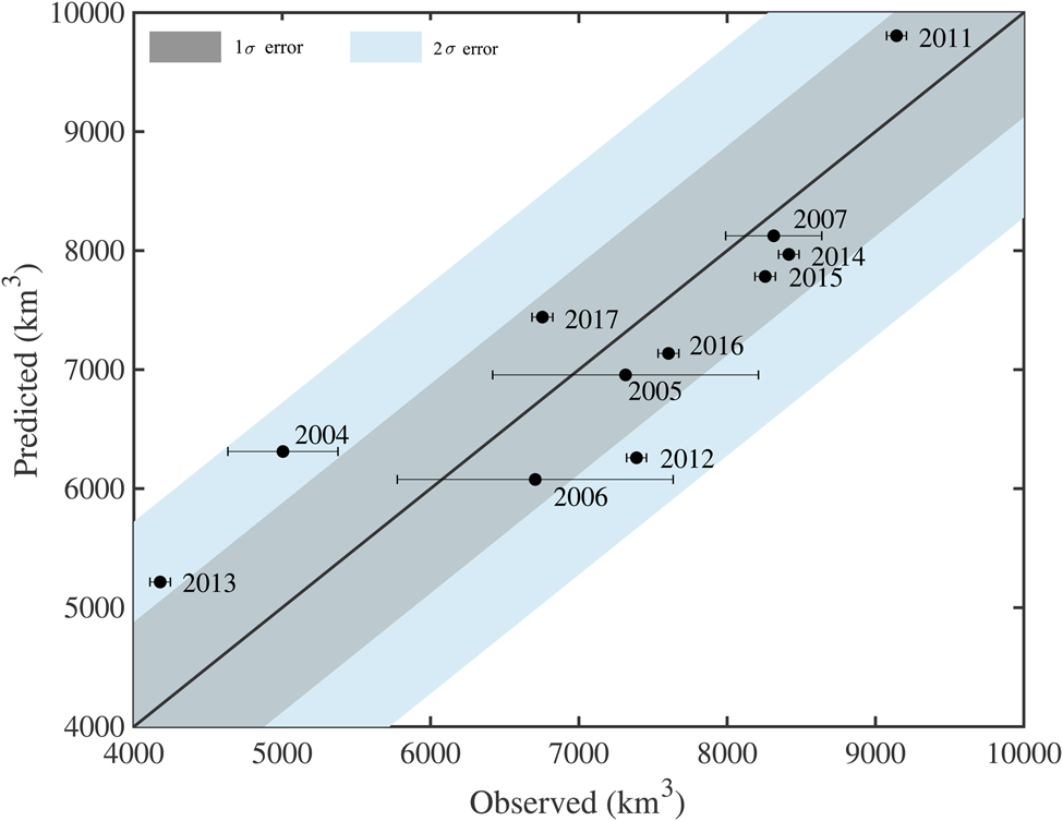
Fig. 4. Comparison plot of observed seasonal ice volume loss (km3) and predicted losses from the bivariate multilinear regression model (utilizing March LWd and mean June/July CRE$_{\rm LW_{\rm d}}$ as predictor variables). Points falling above the black line indicate that modeled values were larger than observed values. Observational uncertainties are plotted along the horizontal axis.
Table 2. Univariate linear regression models with p-values <0.1, listed in order of decreasing R 2 values, and the bivariate regression model using the top two predictors (bottom row)
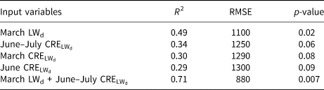
Also shown are root-mean-square errors (RMSE, in km3), and p-values.
The regression model's performance and coefficients are not significantly altered when tested on the 9-year subset (excluding the most recent years, 2016 and 2017), with similar relationships to March LWd (R 2 = 0.56, p = 0.02), June + July CRE$_{\rm LW_{\rm d}}$ (R 2 = 0.32, p = 0.11), and a strong fit in the bivariate linear regression model (R 2 = 0.74, p = 0.02, with a RMSE of 940 km3 vs 1650 km3 RMS deviation from the 9-year mean). We note that given the small sample size and use of several tested independent variables, interpretations of relationships with p-values near 0.1 are limited. A relationship meeting the p = 0.10 threshold in and of itself may occur by chance rather than through related physical mechanisms. However, the consistency of the most correlated independent variables and their respective levels of significance in both the full and subset samples improve our confidence in their importance to sea-ice variability. The resulting predicted 2016 and 2017 values are biased similarly in sign to the predicted values from the 11-year model, with the model under-predicting volume loss in 2016 and over-predicting loss in 2017. The mean bias for these two years (600 km3) is comparable to the bias using the 11-year model (575 km3). The physical mechanisms connecting these two radiative variables to interannual variability in sea-ice melt are discussed in the following sections.
Radiative impact of March LWd on melt onset
March marks an important transition period in the Arctic between an insolation-free winter and the return of incident solar radiation. As shortwave radiation returns to the surface energy budget, the CRENet flux begins to decline, due to the increase in magnitude of CRESW which is opposite in sign to CRELW (Fig. 1). CRESW increases in magnitude until the shortwave component eventually dominates CRELW in June and July. March also marks the initial melt onset of snow on sea ice. The timing of melt onset exhibits a strong meridional gradient (Markus and others, Reference Markus, Stroeve and Miller2009), with regions of melt onset in March limited to near the ice edge, most notably in the Barents and Kara Seas. Over the satellite era, the timing of this melt is trending toward earlier onset (Bliss and Anderson, Reference Bliss and Anderson2018). As melt occurs, albedo is reduced over the melting snow and ice surfaces due to the changing crystalline structure within the surface snowpack (Maksimovich and Vihma, Reference Maksimovich and Vihma2012). The reduced albedo, combined with the seasonal return of shortwave radiation, supports an ice-albedo warming feedback at the surface (Gorodetskaya and Tremblay, Reference Gorodetskaya, Tremblay, DeWeaver, Bitz and Tremblay2013) and increases the total solar energy absorbed by the ice–ocean system in the spring and summer months (Stroeve and others, Reference Stroeve, Markus, Boisvert, Miller and Barrett2014). However, Maksimovich and Vihma (Reference Maksimovich and Vihma2012) found that melt onset in the Arctic is triggered primarily by changes in downwelling longwave radiation, with this flux explaining up to 90% of the melt onset variance in some regions of the central Arctic. Downwelling longwave fluxes were found to be particularly important for melt onset in regions of the sea-ice pack that melt earliest in the spring, with positive longwave anomalies often caused by the remote transport of heat and moisture fluxes to the Arctic (Mortin and others, Reference Mortin2016). While downwelling longwave radiation is not necessarily caused by cloud presence (e.g. enhanced downwelling longwave radiation and melt onset can be triggered by warm air advection (Liu and Schweiger, Reference Liu and Schweiger2017)), increased cloud fraction during the early spring months, when clouds are behaving as near black body emitters (Shupe and Intrieri, Reference Shupe and Intrieri2004), can enhance downwelling longwave radiation at the surface, initiating earlier and more widespread melt.
We test the relationship between CERES-EBAF March LWd and SMMR SSM/I day of melt onset over the 2000–2017 period, computing the correlation for each gridpoint over the 18-year period. We find that significant correlations are limited to a few small regions, mainly located near the perimeter of the analysis domain, along the edges of the central Arctic basin (Fig. 5). It is worth noting that only a small fraction of the central Arctic domain typically begins surficial melting in March and early April, as calculated from average day of melt onset from the SMMR SSM/I brightness temperature product. We overlay these regions with stippling in Figure 5. The concentrated region of early occurring melt in the North Atlantic coincides with the largest region of high correlations between March LWd and melt onset, suggesting that regions with early melt onset are sensitive to variability in early spring downwelling longwave radiation. This result is consistent with those discussed in Mortin and others (Reference Mortin2016), who found that the presence of high moisture clouds, which enhance the greenhouse effect, is crucial to early melt onset in the spring.
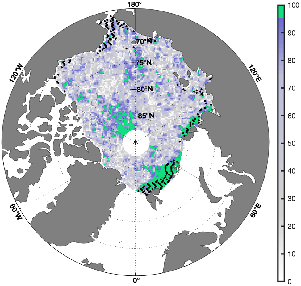
Fig. 5. Confidence levels of the time correlations between day of melt onset and March LW d over the 2000–2017 period across the IS/JPL domain. Colors correspond to the confidence level, with regions in green denoting areas where the two variables are correlated with the 95% confidence level. Regions that undergo melt onset in March and April, calculated from average day of melt onset over the study period, are indicated by black stippling.
We note that radiative forcing in March may not be directly related to the magnitude of melt, but could rather explain some fraction of the interannual variability in ice growth/thickening between March and April. While melt onset begins in March over areas on the domain's periphery, total ice volume integrated over the study domain continues to increase from March to April, when it reaches an annual maximum volume, as shown both in the modeled PIOMAS and observed CS-2 ice volume results (Fig. 3). Mean ice volume growth from March to April over the 2000–2017 period, calculated from PIOMAS data, is 830 (±150) km3. Similarly, ice volume between March and April, calculated from CS-2 over the 2011–2017 period, increases on average by 945 (± 250) km3. We find a significant negative correlation (R 2 = 0.23, p = 0.045) between PIOMAS-derived ice volume growth and CERES-EBAF March LWd. The correlation increases when excluding ICESat observational years and using only CS-2-derived volume changes (R 2 = 0.45), but the relationship is not significant to the 95th percentile due to the small sample size of CS-2 observations (n = 7; p = 0.09). These results suggest that enhanced downwelling longwave radiation in March may reduce the rate of sea-ice thickening (via mitigating surface heat losses) between March and April over interior regions that have not yet undergone surficial melt. Therefore, sea ice would be thinner leading into the melt season. These findings are consistent with conclusions from Maksimovich and Vihma (Reference Maksimovich and Vihma2012), who found that latent and sensible heat fluxes play an important role in modulating the timing of melt onset primarily through their ability to reduce the amount of surface heat loss during the early spring. Similarly, Letterly and others (Reference Letterly, Key and Liu2016) found that enhanced springtime LWd has implications for ice thickness that extends well into the main melt season months through positive feedbacks.
Enhanced sensitivity to CRE during months of greatest ice volume melt
In the absence of observational sea-ice thickness and volume data from May through September, we use monthly PIOMAS estimates to constrain the timing and magnitude of ice loss during these months. Month-to-month reductions in ice volume over the study domain typically occur from April–September, with net gain occurring from March to April, and September to October. The greatest volume losses occur from June to July and from July to August, with an average volume reduction of 4400 and 2740 km3, respectively. The volume losses in June/July dominate volume changes during the rest of the melt season; thus, changes to the surface radiative budget during this period can be expected to have more pronounced impacts on the magnitude of total seasonal ice volume losses than in other months.
June–July CRE$_{\rm LW_{\rm d}}$ is negatively correlated with seasonal volume losses, meaning that greater downwelling fluxes are associated with decreased melt. This may suggest that the presence of clouds during periods of peak solar insolation cools the surface by reflecting downwelling shortwave radiation. This is further discussed in Choi and others (Reference Choi2014), where variability in cloud cover during June was found to have a large impact on the variability of the absorbed solar radiation at the surface. However, we do not find any significant correlations between shortwave variables during this June–July period and ice volume losses in these months, though only modeled volume changes from PIOMAS are available for testing due to a lack of summertime ice volume observations. Therefore, while variability in radiative fluxes in June/July have the greatest potential to alter volume losses due to the large magnitude of melt during these months, the specific mechanism linking June–July CRE$_{\rm LW_{\rm d}}$
 to ice volume reductions is less clear.
Impact of ice dynamics
In addition to the thermodynamic processes investigated here, large-scale sea-ice dynamics are another component of interannual variability in sea-ice volume losses. Sea-ice advection through Fram Strait, the largest outlet for sea-ice transport, exported 217 km3 month−1 over the ICESat period (Spreen and others, Reference Spreen, Kern, Stammer and Hansen2009), or ~1500 km3 over the 7-month melt season defined in this study, which is >20% of the mean ICESat seasonal volume losses. Anomalies in sea-ice velocity can impact late-season sea-ice concentration (Smedsrud and others, Reference Smedsrud, Halvorsen, Stroeve, Zhang and Kloster2017), and amplify or dampen volumetric changes from radiative forcing alone. Previous studies have analyzed the contribution of atmospheric forcing on sea-ice extent (Rigor and others, Reference Rigor, Wallace and Colony2002; Deser and Teng, Reference Deser and Teng2008; Wang and others, Reference Wang2009). Interannual variability in summer sea-ice extent has been linked to processes enhancing transpolar drift, such as synoptic events (Zhang and others, Reference Zhang, Lindsay, Steele and Schweiger2008; Screen and others, Reference Screen, Simmonds and Keay2011) and shifts in climate indices such as the springtime Arctic Dipole (Zhang, Reference Zhang2015).
Here, we do not directly assess the contribution of dynamic forcing to sea-ice volume losses but highlight two specific years, one each with higher-than-predicted and lower-than-predicted volume losses. We find that anomalous sea-ice advection patterns in these years (2012 and 2013) heavily influenced net ice volume losses, impacting the skill of the regression model. In 2013, CS-2 observed a minimum ice volume loss of 4180 km3, something of an outlier in the time series (see Fig. 3) that has also been noted in previous study (Tilling and others, Reference Tilling, Ridout, Shepherd and Wingham2015). The lowest March LWd during observational years also occurred in 2013, which is reflected in the low predicted volume losses from the 1-variable model. We would expect lower volume losses in years with reduced March LWd because there is less longwave energy available to warm the surface, and thus greater volume increases in the central Arctic from March to April. Indeed, volume growth from March to April in 2013 (1160 km3) was well above the CS-2 average of 945 (±250) km3.
2013 is also the most poorly-predicted year by the to p-rated univariate regression model and the third-worst for the bivariate regression model (Table 3). While high values of June-July CRE$_{\rm LW_{\rm d}}$ (i.e. net surface cooling) resulted in the 2-variable model predicting only 5220 km3 of seasonal ice loss, this value was still well above the observed loss of 4180 km3 (Table 2). One explanation for the anomalously low ice melt in 2013 compared to the prediction by the multilinear regression model is the anomalous large scale advection pattern that year. Tilling and others (Reference Tilling, Ridout, Shepherd and Wingham2015) show that low melt in 2013 was due to the retention of thick sea-ice northwest of Greenland. We similarly show that anomalous advection patterns likely played a role in retaining thicker ice in the central Arctic basin. Our analyses of PIOMAS-modeled sea-ice advection climatology show that during a typical June, anticyclonic flow in the Beaufort Sea feeds into the transpolar drift, leading to export through Fram Strait (Fig. 6a). However, in 2013, a strong cyclonic pattern dominated sea-ice advection in the central Arctic, reducing the ice loss through Fram Strait (Fig. 6b).
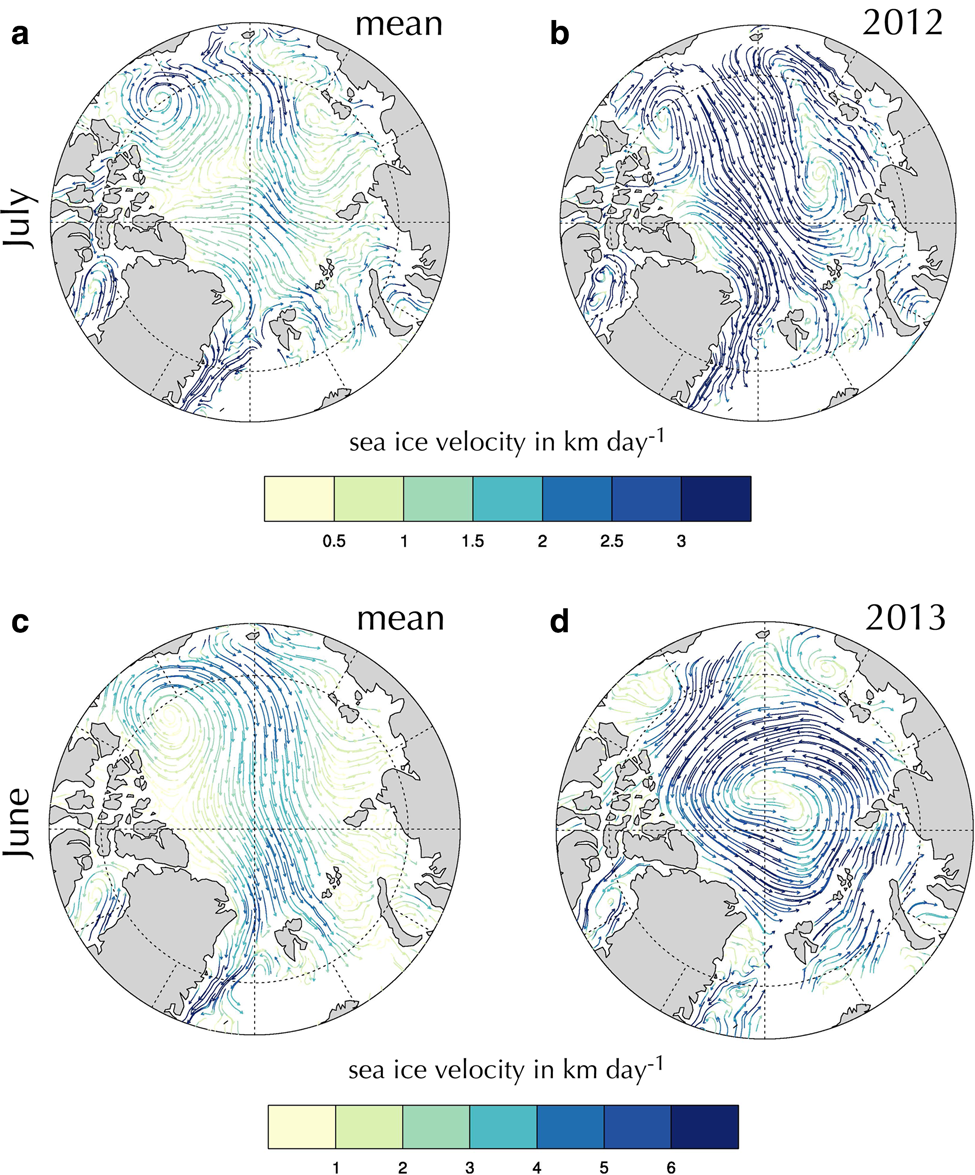
Fig. 6. (a) Mean sea-ice velocity (in km d−1) during the month of July, calculated from PIOMAS data over the 2000–2017 period. (b) Ice velocities during July 2012. The velocity patterns favor enhanced ice export through the Fram Strait relative to the average. (c) Mean sea-ice velocity (in km d−1) during the month of June, calculated from PIOMAS data over the 2000–2017 period. Mean velocities resemble anticyclonic flow and favor ice export through the Fram Strait. (d) Ice velocities during June 2013. The strong cyclonic pattern in the central Arctic reduced ice export through the Fram Strait. Note that the color bar is scaled by 2 for ice velocities in (c) and (d).
Table 3. Observed and predicted sea-ice volume loss from the top univariate and from the bivariate (March LWd + June–July CRE$_{\rm LW_{\rm d}}$ ) regression models
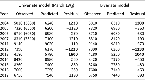
Actual sea-ice volume loss, predicted volume loss and residuals are in units of km3. ICESat-derived volumes prior to the bias corrections discussed in the ‘Methods’ section are given in parentheses. The three largest residuals for each model are highlighted in bold.
The bivariate regression model shows errors greater than σ in two other years, 2004 and 2012 (Fig. 4), which are also associated with the second and third largest errors of the univariate model. 2004 does not show obvious springtime anomalous advection patterns like 2013, and the timing of volume change anomalies is particularly challenging to identify due to the limited temporal data availability during the ICESat era. Ice loss in 2012, however, is well documented as the result of a strong late summer cyclone over the central Arctic (Parkinson and Comiso, Reference Parkinson and Comiso2013; Petty and others, Reference Petty2018). Through June, monthly volume changes during 2012 were near average, but transitioned to ice advection patterns favoring ice export in July (Fig. 6). Anomalously high volume losses in July due to enhanced export through the Fram Strait, paired with a strong cyclone in August 2012 (Parkinson and Comiso, Reference Parkinson and Comiso2013), likely contributed to higher-than-predicted ice volume losses. Finally, we note that in addition to the dynamic processes discussed here, other thermodynamic components likely also impact sea-ice loss. In the case of 2012, for example, a strong August cyclone also brought moisture and warm near-surface air temperatures to affected sea-ice regions, which compounds dynamic ice export and divergence (Parkinson and Comiso, Reference Parkinson and Comiso2013).
Conclusions
We find that large-scale monthly average radiative components can serve as predictive tools for estimating the total seasonal ice volume loss from March–October. Specifically, March LWd and June–July CRE$_{\rm LW_{\rm d}}$ jointly can account for >70% of the observed volume loss variability. These variables are successful predictors because of their impact on the timing of melt onset, which begins in March, and on the period of highest melt rates in June and July. Our results are similar to those of Kapsch and others (Reference Kapsch, Graversen, Tjernström and Bintanja2016), who found that springtime downwelling longwave radiation significantly impacted September sea-ice extent. They further noted that downwelling longwave radiation in June and July is important because much of the surface is at or near the melting point, and radiative anomalies can therefore impart a more rapid reduction in the ice surface albedo through the formation and expansion of melt ponds. The two radiative fluxes identified here as most highly correlated with ice volume loss, and the respective sign of their relationship to sea-ice volume loss, are also in general agreement with a localized study of cloud impact on sea ice near Barrow, AK (Cox and others, Reference Cox2016), which found that a combination of positive longwave cloud anomalies in the early spring, followed by a later transition to negative longwave anomalies in early summer, are associated with low sea ice (high melt) years. Huang and others (Reference Huang2019) find that downwelling longwave radiation in April and June is most closely correlated with September sea-ice extent, with other studies attributing favorable summer sea-ice melt conditions (enhanced downwelling longwave radiation resulting from heat and moisture fluxes in the lower atmosphere) to, in part, teleconnections with Pacific sea surface temperatures (Baxter and others, Reference Baxter2019; Ding and others, Reference Ding2019; Bonan and Blanchard-Wrigglesworth, Reference Bonan and Blanchard-Wrigglesworth2020). We find that March conditions are more important than those in April for seasonal sea-ice development. Note, however, that our focus is on volumetric, rather than areal, changes in sea ice. Enhanced downwelling longwave radiation suppresses ice thickening over a domain that is typically 100% ice covered in March, and therefore has a less direct impact on sea-ice extent. Our regression results suggest that seasonal ice volume changes are largely insensitive to variability in shortwave fluxes, with a lack of any significant correlations between the monthly downwelling shortwave fluxes and net volume losses. This is consistent with conclusions by Kapsch and others (Reference Kapsch, Graversen, Tjernström and Bintanja2016), who argued that high surface albedo in the spring, particularly over the central Arctic Basin as used in this study, reduces the impact of interannual variability in downwelling shortwave radiation.
Radiative fluxes and thermodynamic properties near the sea-ice surface, however, are only one component of seasonal sea-ice evolution. Strong advection anomalies can overshadow the impact of radiative fluxes on seasonal ice volume loss, as was the case in 2013 and likely in 2012, by changing the level of sea-ice export from the Arctic. Our model poorly predicted ice volume losses in 2013, a season which has also proved challenging for other statistical, thermodynamic-based models due to the anomalous dynamic patterns (Ionita and others, Reference Ionita, Grosfeld, Scholz, Treffeisen and Lohmann2019), as well as for the complex PIOMAS model. The active role of sea-ice advection in modulating changes in sea-ice volume, and its dependency on weather conditions, remains a challenge for sea-ice forecasts. During dynamically typical years, however, we show that downwelling longwave fluxes in March combined with cloud radiative forcing in June and July play an important role in the interannual variability in sea-ice volume loss in the central Arctic Basin. Previous studies (Kapsch and others, Reference Kapsch, Graversen, Economou and Tjernström2014) show that statistical models have the potential to predict September sea-ice conditions with comparable skill to coupled ice–ocean models over large domains. Knowledge of these specific radiative fluxes, along with careful consideration of patterns of ice motion, can form the basis of fall Arctic sea-ice volume predictions.
Acknowledgments
All data used in our study were acquired from publicly available data repositories. We obtained ICESat sea-ice thickness from NASA JPL (http://rkwok.jpl.nasa.gov/icesat/download.html), CryoSat-2 sea-ice thickness data from AWI (Hendricks and others, Reference Hendricks, Ricker and Helm2016) accessed through the online data portal at https://data.seaiceportal.de/gallery/index_new.php. PIOMAS version 2 from the APL Polar Science Center was downloaded at http://psc.apl.uw.edu/research/projects. SMMR SSM/I sea-ice concentration and melt onset data are obtained through NSIDC at https://doi.org/10.5067/IJ0T7HFHB9Y6 and https://nsidc.org/data/nsidc-0105, respectively. Finally, CERES-EBAF surface radiative fluxes can be subset and downloaded through the NASA Langley site (https://ceres.larc.nasa.gov/products-info.php?product=EBAF). We thank the reviewers and scientific editor for their valuable comments that improved the manuscript.


 Open access

