


INTRODUCTION
The large-scale structure of ice sheets and glaciers (e.g. thickness and internal layering) can be characterized using passive seismology (Podolskiy and Walter, Reference Podolskiy and Walter2016; Aster and Winberry, Reference Aster and Winberry2017). Several approaches of exploiting the ambient seismic wavefield, which mostly consists of surface waves (Bonnefoy-Claudet and others, Reference Bonnefoy-Claudet, Cotton and Bard2006b), have been developed and applied for this purpose. Using the properties of surface waves is less precise than reflection seismics (e.g. Thyssen and Ahmad, Reference Thyssen and Ahmad1969; Hofstede and others, Reference Hofstede2018) or radio-echo sounding (also called radar, e.g. Plewes and Hubbard, Reference Plewes and Hubbard2001), let alone drilling ice boreholes (e.g. Sugiyama and others, Reference Sugiyama2008), but is easier to perform. Furthermore, seismometers could allow the long-term monitoring of englacial or subglacial properties, which would be particularly useful for the surveillance of avalanching or calving glaciers. Compared with active surface wave methods (e.g. Armstrong, Reference Armstrong2009; Ivanov and others, Reference Ivanov, Miller, Peterie and Tsoflias2014), passive measurements potentially reach larger depths due the lower frequency content of the natural noise field, although they may lack energy to characterize the top meters. Therefore, they could potentially reveal the bed's properties, such as the presence or absence of sediment and its mechanical properties (Picotti and others, Reference Picotti, Francese, Giorgi, Pettenati and Carcione2017).
Most of the seismological methods used here are rooted in engineering seismology, where they are employed for the characterization of seismic station sites, e.g. on sediment basins, bedrock outcrops or unstable rock masses (e.g. Picozzi and others, Reference Picozzi2009; Foti and others, Reference Foti, Parolai, Albarello and Picozzi2011; Michel and others, Reference Michel2014; Poggi and others, Reference Poggi, Ermert, Burjánek, Michel and Fäh2015, Reference Poggi, Burjánek, Michel and Fäh2017; Martorana and others, Reference Martorana2018). From this established field of research, it is well known that geometrical effects can have a dominant influence on the wavefield when the site violates the common assumption that the subsurface is a 1-D horizontally layered medium. Geometrical effects in this sense are modifications of the seismic wavefield due to cracks and faults (Burjánek and others, Reference Burjánek, Moore, Molina and Fäh2012), surface (Buech and others, Reference Buech, Davies and Pettinga2010; Burjánek and others, Reference Burjánek, Edwards and Fäh2014) and bedrock topography (Bard and Bouchon, Reference Bard and Bouchon1985; Roten and others, Reference Roten, Fäh, Cornou and Giardini2006; Ermert and others, Reference Ermert, Poggi, Burjánek and Fäh2014).
In this paper, we investigate the effects of geometry on the seismic wavefield of Alpine glaciers, especially how resonance effects can be interpreted and utilized, but also how they can interfere with measurements. We calculate horizontal-to-vertical spectral ratios (HVSR or H/V ratios) from all glaciers and compare it to synthetic estimates from 1-D models constructed from independent glacier thickness estimates. We further analyze the polarization of the wavefield to determine whether we have higher order (2-D or 3-D) resonance, the occurrence of which can explain why HVSR does not match the predictions using 1-D models. Modal analysis finally allows us to further describe the deformation of the resonating bodies.
Previous studies of geometrical effects
Geometrical effects can be divided into local and global effects. Typical local effects in sedimentary valleys are edge-generated surface waves, which are broadband waves caused by constructive interference of the direct S-wave with waves diffracted due to the basin geometry (Kawase, Reference Kawase1996; Cornou and Bard, Reference Cornou and Bard2003; Hallier and others, Reference Hallier, Chaljub, Bouchon and Sekiguchi2008). Global effects are resonances due to normal modes of a well-defined geological (or glaciological) structure, occurring at discrete frequencies (Fig. 1). In this paper, we will only consider the latter, as the former are hardly seen in the ambient vibrations due to the distributed unknown location of the sources.
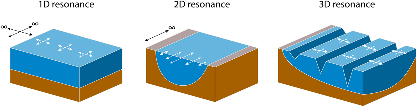
Fig. 1. Schematic cartoon of the different resonances (1-D, 2-D, 3-D). White arrows depict the ground motion, and black arrows show the dimensions assumed to have infinite extent (after Roten and others (Reference Roten, Fäh, Cornou and Giardini2006)). The particle motion is omni-directional in the 1-D case, but has a preferred orientation in the 2-D and 3-D case, which can be detected by polarization analysis.
One-dimensional resonance of S-waves is particularly strong for a soft layer on top of a rigid layer. At about the same frequency, Rayleigh waves show a peak in ellipticity and Love waves have their strong Airy phase. These phenomena cause the horizontal motion to be larger than the vertical motion, which is exploited in the popular HVSR or H/V ratios method for the analysis of ambient vibrations. To obtain the H/V curve, the averaged frequency spectra of the horizontal components of a single station are divided by the spectrum of the vertical component. The frequency, at which the H/V curve has a peak, can be used as an estimate of the fundamental resonance frequency of a horizontally layered 1-D medium (Bonnefoy-Claudet and others, Reference Bonnefoy-Claudet, Köhler, Cornou, Wathelet and Bard2008). In a one-layer over bedrock system, the thickness of the resonating layer can be estimated (e.g. Kramer, Reference Kramer2014) with
 $$ H = {V_{\rm s} \over {4f_0}},$$
where H is the thickness of the resonator, V s is the shear wave velocity and f 0 the resonance frequency. Additionally, the H/V curve can be inverted to obtain the subsurface structure (e.g. Fäh and others, Reference Fäh, Kind and Giardini2003; Bonnefoy-Claudet and others, Reference Bonnefoy-Claudet2006a; García-Jerez and others, Reference García-Jerez, Pina-Flores, Sánchez-Sesma, Luzón and Perton2016). This method has also previously been applied to glacial settings, as we will discuss below.
Two-dimensional resonance refers to the possibility of standing waves between valley walls (Fig. 1). It was already identified by Tucker and King (Reference Tucker and King1984) and modeled by Bard and Bouchon (Reference Bard and Bouchon1985), who explore the case of a sediment-filled valley using a simple numerical model. They derived a relationship that predicts whether 2-D resonance occurs based on the velocity contrast and the shape ratio. The latter is defined as the ratio h/l, i.e. the maximum sediment thickness (h) over the valley half-width (l) for sine-shaped valleys. For other valley shapes, the ‘equivalent’ shape ratio (h/2w) is used, where 2w is the total width over which the sediment thickness is more than half its maximum value. With knowledge of the subsurface structure, it is therefore possible to predict the existence of 2-D resonances, e.g. for a deep sediment-filled valley with a strong velocity contrast between sediment and bedrock. In other cases, the valley shape and/or the velocity contrast are not known a priori, and the seismic waveforms have to be analyzed. In any case, this description of the phenomena is simplified and real cases are likely more complex (see e.g. Michel and others (Reference Michel2014)).
The glacially carved Rhone valley, Switzerland, is one example of a deep sediment-filled valley and has been intensely studied. Roten and others (Reference Roten, Fäh, Cornou and Giardini2006) measured ambient vibrations along a dense seismometer profile and investigated its resonance behavior. Existing high-resolution active seismic data allowed determination of the velocity contrast as well as the shape ratio, showing that their site is clearly located in the domain of 2-D resonance. Whereas the 1-D resonance frequency would be around 0.2 Hz, they showed that the seismic wavefield is dominated by standing waves caused by 2-D resonance in higher frequencies (0.25–0.5 Hz). Thus, they conclude that a 1-D analysis is insufficient to describe the response of this site and might lead to wrong conclusions. Ermert and others (Reference Ermert, Poggi, Burjánek and Fäh2014) and Poggi and others (Reference Poggi, Ermert, Burjánek, Michel and Fäh2015) used array recordings of ambient vibrations at this site to identify several resonance modes, including higher modes using polarization analysis and frequency domain decomposition (FDD) (see ‘Methods’ section).
Analyzing the polarization of the wavefield allows to recognize geometrical resonances also at sites without axisymmetry and thus potentially displaying 3-D resonance patterns (Fig. 1). Burjánek and others (Reference Burjánek, Gassner-Stamm, Poggi, Moore and Fäh2010) introduced this method as time-frequency-dependent polarization analysis (TFPA). TFPA characterizes the ground motion for each time step and frequency by an ellipse, described by the strike, the dip and the circularity (the latter is called ellipticity by Burjánek and others (Reference Burjánek, Gassner-Stamm, Poggi, Moore and Fäh2010)). It has since been applied to seismic noise on unstable rock slopes (Burjánek and others, Reference Burjánek, Moore, Molina and Fäh2012; Kleinbrod and others, Reference Kleinbrod, Burjánek and Fäh2017a,Reference Kleinbrod, Burjánek, Hugentobler, Amann and Fähb) and is used for seismic site characterization (Michel and others, Reference Michel2014). Burjánek and others (Reference Burjánek, Gischig, Moore and Fäh2017) used it for monitoring of an unstable rock slope.
Previous applications in a glaciological context
Passive seismology is becoming increasingly popular in glacial applications (Podolskiy and Walter, Reference Podolskiy and Walter2016). Below, we give an overview of studies analyzing ambient seismic vibrations relevant for our seismic site effect study in a glacial context.
Lévêque and others (Reference Lévêque, Maggi and Souriau2010) calculate H/V ratios for five stations on Dome C, Antarctica. From these, they infer the thickness of the uppermost unconsolidated snow layer (around 30 m). Zhan and others (Reference Zhan, Tsai, Jackson and Helmberger2014) use data from Amery Ice Shelf, Antarctica, to calculate noise correlation functions. The spectral ratios derived from these show several peaks, which are interpreted as P-wave resonances in the water layer below the ice shelf (‘cavity’), and provide an estimate of the water-column thickness.
Picotti and others (Reference Picotti, Francese, Giorgi, Pettenati and Carcione2017) use seismic noise records from several Alpine glaciers and from Whillans Ice Stream (Antarctica) to calculate H/V curves, which they then invert for the bedrock depth. They validate their results using independent measurements such as radio-echo sounding and geoelectric and active seismic profiling. Whereas their results from the Alpine glaciers are promising, they are unable to estimate the bedrock depth on Whillans Ice Stream. They argue that the deformable bedrock in addition to waves trapped in the firn layer lead to resonance not related to the bedrock.
Yan and others (Reference Yan2018) calculate H/V spectral ratios from 65 stations across the Antarctic Ice Sheet and obtain depths comparable to the well-known Bedmap 2 dataset (Fretwell and others, Reference Fretwell2013). Their inversions reveal that the Antarctic Ice Sheet is best approximated by two ice layers over bedrock, where the lower ice layer has a reduced shear wave velocity compared with data the upper ice layer due to the presence of unfrozen liquids along the ice grain boundaries (Wittlinger and Farra, Reference Wittlinger and Farra2015). This is in agreement with Wittlinger and Farra (Reference Wittlinger and Farra2012) as well as Wittlinger and Farra (Reference Wittlinger and Farra2015), who use receiver functions to also describe the Antarctic Ice Sheet as a two-layer ice medium over bedrock.
Here, we build on this existing work and further analyze how the ambient wavefield differs on glaciers with a more complex englacial structure or glacier bed, essentially on glaciers which do not fulfill the assumption of a horizontally layered 1-D medium. We first briefly discuss the methods employed here, followed by three examples of glaciers in the Swiss Alps, and how their data can be interpreted in terms of glacial characteristics.
METHODS
Horizontal-to-vertical spectral ratios
As shortly outlined in the introduction, HVSR or H/V are the ratios of the frequency spectra of the horizontal and the vertical components of a single station. They have been widely used for seismic site characterization on an empirical basis (e.g. SESAME, 2004). Several different theories can explain observations in specific situations (e.g. by assuming that the curve represents Rayleigh wave ellipticity, or SH-wave resonance, sometimes with contributions from the Airy phase of Love waves). However, a unifying theory considering the full wavefield was debated for a long time (see review of Lunedei and Malischewsky, Reference Lunedei, Malischewsky and Ansal2015).
Substantial progress in the theoretical understanding of HVSR has been made recently by employing the diffuse field assumption (DFA). It allows to link the HVSR of ambient seismic noise (assumed to be an equipartitioned diffuse field) to seismic interferometry. Therefore, it can be shown that the imaginary part of the elastic Green's function can be retrieved from the autocorrelation of noise recorded at one station (Sánchez-Sesma and others, Reference Sánchez-Sesma2011; Kawase and others, Reference Kawase, Matsushima, Satoh and Sánchez-Sesma2015; Lontsi and others, Reference Lontsi, Sánchez-Sesma, Molina-Villegas, Ohrnberger and Krüger2015; García-Jerez and others, Reference García-Jerez, Pina-Flores, Sánchez-Sesma, Luzón and Perton2016; Piña-Flores and others, Reference Piña-Flores2017; Sánchez-Sesma, Reference Sánchez-Sesma2017). Using three-component recordings, the full elastic Green's tensor can be retrieved. Its diagonal elements related to the horizontal components are then divided by the one related to the vertical component to obtain the HVSR.
This framework has also found new practical applications in environmental seismology, for example, for volcanoes (Spica and others, Reference Spica2015), or ice sheets (Yan and others, Reference Yan2018). Perton and others (Reference Perton, Spica and Caudron2018) show that using the DFA, also complex geometries such as a laterally heterogeneous crater wall, can be inverted for. Finally, it should be kept in mind that the inversion of HVSR is inherently non-unique, and therefore commonly inverted together with additional data such as dispersion curves of surface waves (Scherbaum and others, Reference Scherbaum, Hinzen and Ohrnberger2003; Fäh and others, Reference Fäh, Stamm and Havenith2008; Michel and others, Reference Michel2014; Piña-Flores and others, Reference Piña-Flores2017).
Here, we divide 4 h of on-ice seismic noise records into windows of 50 s length and 50% overlap to calculate the vertical as well as the horizontal spectra. We then take the quadratic mean of the horizontal components, stack the traces and apply Konno and Ohmachi (Reference Konno and Ohmachi1998) smoothing with a factor of 80. To compare HVSR to the synthetic Rayleigh wave ellipticity, calculated using geopsy (Wathelet, Reference Wathelet2008), we assume equal contribution of Love and Rayleigh waves (both surface wave modes) and multiply the synthetic ellipticity curves by  $\sqrt {2}$ (Fäh and others, Reference Fäh, Kind and Giardini2001).
Wavefield polarization
TFPA combines the complex polarization analysis (Vidale, Reference Vidale1986) with the continuous wavelet transform (e.g. Torrence and Compo, Reference Torrence and Compo1998). It estimates the ground motion for each time step and frequency (Burjánek and others, Reference Burjánek, Gassner-Stamm, Poggi, Moore and Fäh2010, Reference Burjánek, Moore, Molina and Fäh2012, Reference Burjánek, Edwards and Fäh2014). Different wave phases (Rayleigh, P-, S-waves) have different characteristic ground motions, and for Rayleigh waves, the velocity and polarization depend on the sub-surface structure and on the frequency.
TFPA characterizes the ground motion by an ellipse. Three properties of this ellipse – circularity, strike and dip – can then be evaluated to show how strongly and in what direction the wavefield is polarized at what frequency. Circularity, which is called ellipticity in previous papers and should not be confused with Rayleigh wave ellipticity, is 1 for perfectly circular particle motion, and 0 for linear motion. The strike and dip show the direction of maximum polarization, with the strike denoting the azimuth of the major axis of the ellipse toward north, and the dip the inclination of this axis from the horizontal plane. TFPA is more general than azimuth-dependent HVSR (Burjánek and others, Reference Burjánek, Moore, Molina and Fäh2012).
Modal analysis
Modal analysis deals with the analysis of normal modes of a system (especially its resonance frequencies, modal shapes and damping ratios), typically in civil and mechanical engineering to evaluate mechanical structures. Ermert and others (Reference Ermert, Poggi, Burjánek and Fäh2014) and Poggi and others (Reference Poggi, Ermert, Burjánek, Michel and Fäh2015) introduced modal analysis for the study of non-1-D geological structures with application to the Rhone valley. They used the FDD, a relatively simple modal analysis method where the complex spectrum of the responses is separated into individual modes, which each correspond to a single degree of freedom system (Brincker and others, Reference Brincker, Zhang and Andersen2001). Practically, this corresponds to the singular value decomposition of the cross power spectral density (CPSD) matrix of the seismic signal of two or more stations recording simultaneously (e.g. Michel and others, Reference Michel, Guéguen, El, Mazars and Kotronis2010). Datasets not overlapping in time can be combined (resulting in better spatial coverage for modal shapes) provided that a common reference sensor was recording. The results of this analysis are the modes characterized by their resonance frequency and modal shape, which gives the relative amplitude of deformation of the considered measurement points.
APPLICATION TO GLACIERS
We use campaign-based seismic array data from three glaciers in the Swiss Alps (station coordinates can be found in the supplement). Each station consisted of Lennartz LE-3-D sensors with a natural frequency of 1 Hz and Nanometrics Taurus, Nanometrics Centaur or Omnirecs Cube digitizers sampling at 100 Hz or higher. The sensors were either placed in shallow ice boreholes (<4 m depth) or buried in pits within the firn (Table S1). The borehole seismometers were corrected for orientation using low-frequency recordings (<0.4 Hz) of teleseismic events and at least one correctly oriented reference sensor (Poggi and others, Reference Poggi, Fäh, Burjánek and Giardini2012). We analyzed recordings of 2 h for the TFPA and modal analysis, and 4 h for HVSR. Using longer time series did not change our results.
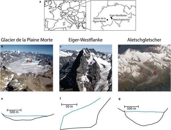
These glaciers cover a range of types and bed geometries. Glacier de la Plaine Morte is a plateau glacier and features only few crevasses. Our second object of study is the avalanching glacier in the Eiger west face (hereafter ‘Eiger-Westflanke’). Aletschgletscher is a typical valley glacier and the longest in the European Alps. In Fig. 2, we show aerial images of these glaciers, along with their bed profiles.

Fig. 2. (a) Map of our study sites. (b)–(d) Aerial images of the glaciers, with the positions of the seismometer studied labeled with red triangles. Marked with a blue line are the profiles shown in the lower part of the figure. (e)–(g) Cross-sections (not vertically exaggerated) through the glaciers, with bed profiles in black and ice surface in blue. Sources: b&c: ETH-Bibliothek Zürich, Bildarchiv/Stiftung Luftbild Schweiz/Fotograf: Swissair Photo AG/LBS_R2-010615 and LBS_R1-970880/CC BY-SA 4.0; d: NASA ISS013-E-77377, e: Grab and others (Reference Grab2018); f: Lüthi (Reference Lüthi1994); g: unpublished measurements by VAW.
Glacier de la Plaine Morte is a glacial plateau on the border between the Swiss cantons of Berne and Valais (Huss and others, Reference Huss, Voinesco and Hoelzle2013). At the location of the network, there are virtually no crevasses, and the glacier flows slowly with velocities <2 cm a−1.
Eiger-Westflanke is a well-known partly cold-based avalanching glacier in the Bernese Alps (Switzerland). Its mass loss occurs mainly via break-off events. A break-off of large ice chunks from this hanging glacier might trigger dangerous combined snow/ice avalanches due to the steep slopes beneath it. Since the train to Jungfraujoch as well as several buildings and hiking paths are in the runout zone of a potential avalanche, the glacier has been monitored for the last two decades (Raymond and others, Reference Raymond, Wegmann and Funk2003; Margreth and others, Reference Margreth2017).
Aletschgletscher is the largest glacier in the European Alps despite the fact that it is rapidly retreating (Jouvet and others, Reference Jouvet, Huss, Funk and Blatter2011). At the site of our array, it is several hundred meters thick and flows at around 100 m a−1 (Preiswerk and Walter, Reference Preiswerk and Walter2018).
From the bed profiles (Fig. 2), we calculate the equivalent shape ratio as proposed by Bard and Bouchon (Reference Bard and Bouchon1985) along with the proposed critical curve, which separates the 1-D regime in the lower left from the 2-D resonance regime in the upper right (Fig. 3). As the shear wave velocity contrast for the sites studied is similar (glacier ice 1.65 km s−1 (Preiswerk and Walter, Reference Preiswerk and Walter2018), bedrock 2.5–3.5 km s−1), the shape ratio of the glacier bed plays a critical role. The uncertainties in the shape ratio are due to the ambiguity in measuring the valley half width and glacier thickness given the shape of the valleys (Fig. 2). Whereas Glacier de la Plaine Morte is not close to the critical curve, Aletschgletscher is slightly below and the Eiger-Westflanke above it. It has to be noted that this is not a sharp boundary between 1-D and 2-D regimes, but an empirically determined transition zone. Also, the glacier bed of Eiger-Westflanke varies within decameters along the direction of flow (no axisymmetry) and cannot be considered as a 2-D but as a 3-D object.
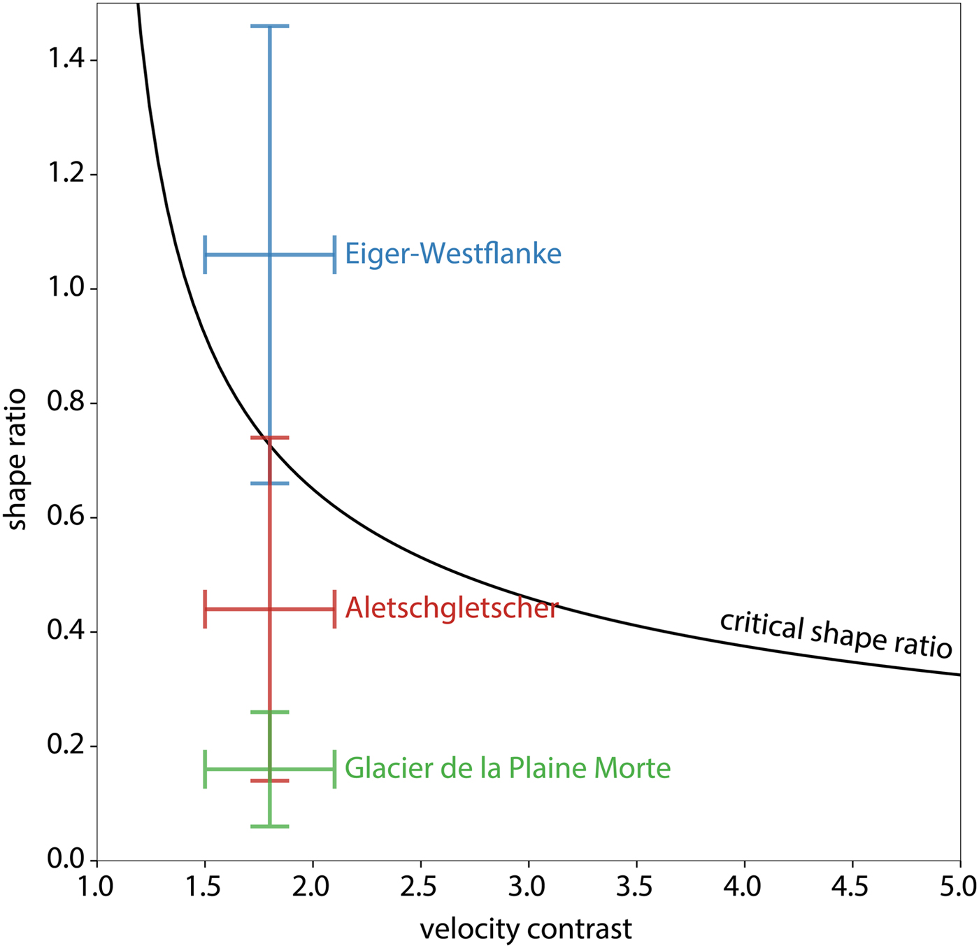
Fig. 3. Prediction of 2-D resonance for the studied glaciers following the approach of Bard and Bouchon (Reference Bard and Bouchon1985): sites with equivalent shape ratios and velocity contrast (between ice and bedrock) above the black critical curve are expected to exhibit 2-D resonance. The velocity contrast ranges are the same for all glaciers (glacier ice 1.65 km s−1 (Preiswerk and Walter, Reference Preiswerk and Walter2018), bedrock 2.5–3.5 km s−1). The estimates of the shape ratios have large uncertainties originating in the ambiguity in measuring the valley half width and glacier thickness given the shape of the valleys (Fig. 2).
The ambient seismic noise on Aletschgletscher mostly consists of surface waves from transient events (icequakes), seismic tremor and anthropogenic noise (Preiswerk and Walter, Reference Preiswerk and Walter2018). The seismic tremor is caused by melt-induced water flow, whereas the origin of anthropogenic noise is probably the Rhone valley with its industrial activity. The seismic sources at the other two glaciers are the same, although in different proportions. A qualitative analysis shows water tremor to be more dominant at Glacier de la Plaine Morte, and icequakes to occur more often on the Eiger-Westflanke compared with Aletschgletscher. To avoid the influence of monochromatic anthropogenic noise and melt-induced local seismic sources as much as possible, we used recordings during night-time for all glaciers.
Glacier de la Plaine Morte - 1-D
The profile through the Glacier de la Plaine Morte (Fig. 2) shows that it is wider than deep. This results in a low shape ratio (Fig. 3).
The HVSR shows a small but well-defined peak around 3.0 ± 0.3 Hz (Fig. 4). Using Eqn 1 and a shear wave velocity of 1.65 km s−1, we obtain a thickness of 140 ± 15 m, which is in the range of radar measurements under the array (130–160 m). Consequently, the observed curves fit well to the theoretical prediction, especially in the more important right flank above the resonance peak (Hobiger and others, Reference Hobiger2013). Additionally, the polarization measurements (Fig. 5) show that there is no preferential orientation of the wavefield, and the circularity is constant across a wide range of frequencies. The modal analysis using FDD shows two orthogonal modes at the same frequency, as expected for 1-D resonance (Fig. S1). This leads to the conclusion that at Glacier de la Plaine Morte, the assumption of 1-D geometry is justified.
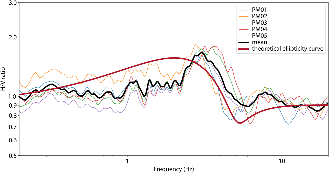
Fig. 4. HVSR of Glacier de la Plaine Morte, showing a peak at 3.0 ± 0.3 Hz on all stations. There is a good agreement to the theoretical Rayleigh wave ellipticity curve for 145 m ice over bedrock, especially in the more important right flank above the resonance peak (Hobiger and others, Reference Hobiger2013).
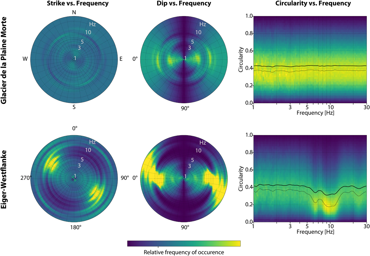
Fig. 5. Time-frequency-dependent polarization analysis (TFPA) of Plaine Morte (PM01, top row), and Eiger-Westflanke (EIG3, bottom row). The radial scale denotes the frequency (Hz). These two stations can be seen as end-member cases: The wavefield is effectively uniform for Glacier de la Plaine Morte, whereas it is polarized perpendicular to the dominant crevasses between 6 and 9 Hz at Eiger-Westflanke.
Eiger-Westflanke - 3-D
Due to its particular setting and location, the Eiger-Westflanke has a distinct geometry. The orientation of the dominant deep crevasses (striking Northeast - Southwest) is orthogonal to the direction of flow (to the Northwest, Fig. 7). Additionally, the bedrock is deeply incised and can therefore not be approximated by a 1-D shape (Lüthi, Reference Lüthi1994; Lüthi and Funk, Reference Lüthi and Funk1997). This leads to a shape ratio above the critical curve (Fig. 3).
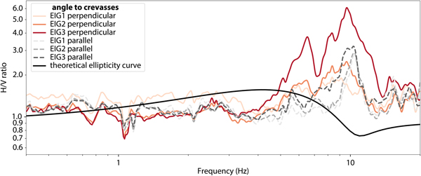
The HVSR curves do not fit to the predicted theoretical ellipticity curve (Fig. 6). This is not surprising, as 1-D models (such as a thickness estimation using Eqn 1) cannot be used for 2-D or 3-D sites (Roten and others, Reference Roten, Fäh, Cornou and Giardini2006). Furthermore, there is also a strong azimuth dependence in the HVSR curves, seen by the difference between HVSR measured parallel and perpendicular to the crevasses (Fig. 6). Consequently, we also observe a strong polarization of the wavefield using TFPA (Fig. 5). The dominant direction of ground motion is found to be parallel to the predominant direction of deformation, and slightly tilted from the horizontal. The polarization is therefore perpendicular to the crevasses.
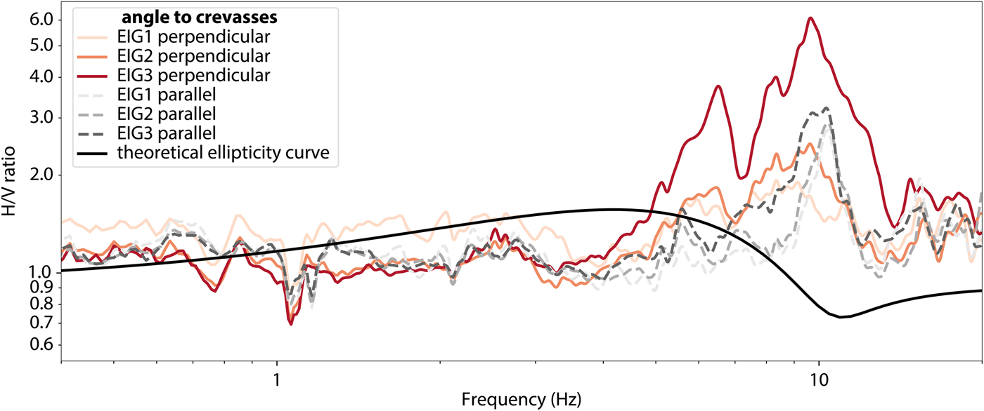
Fig. 6. HVSR of Eiger-Westflanke with a theoretical ellipticity curve for 70 m ice over bedrock. As expected, the observed curves differ substantially from the theoretical predictions.
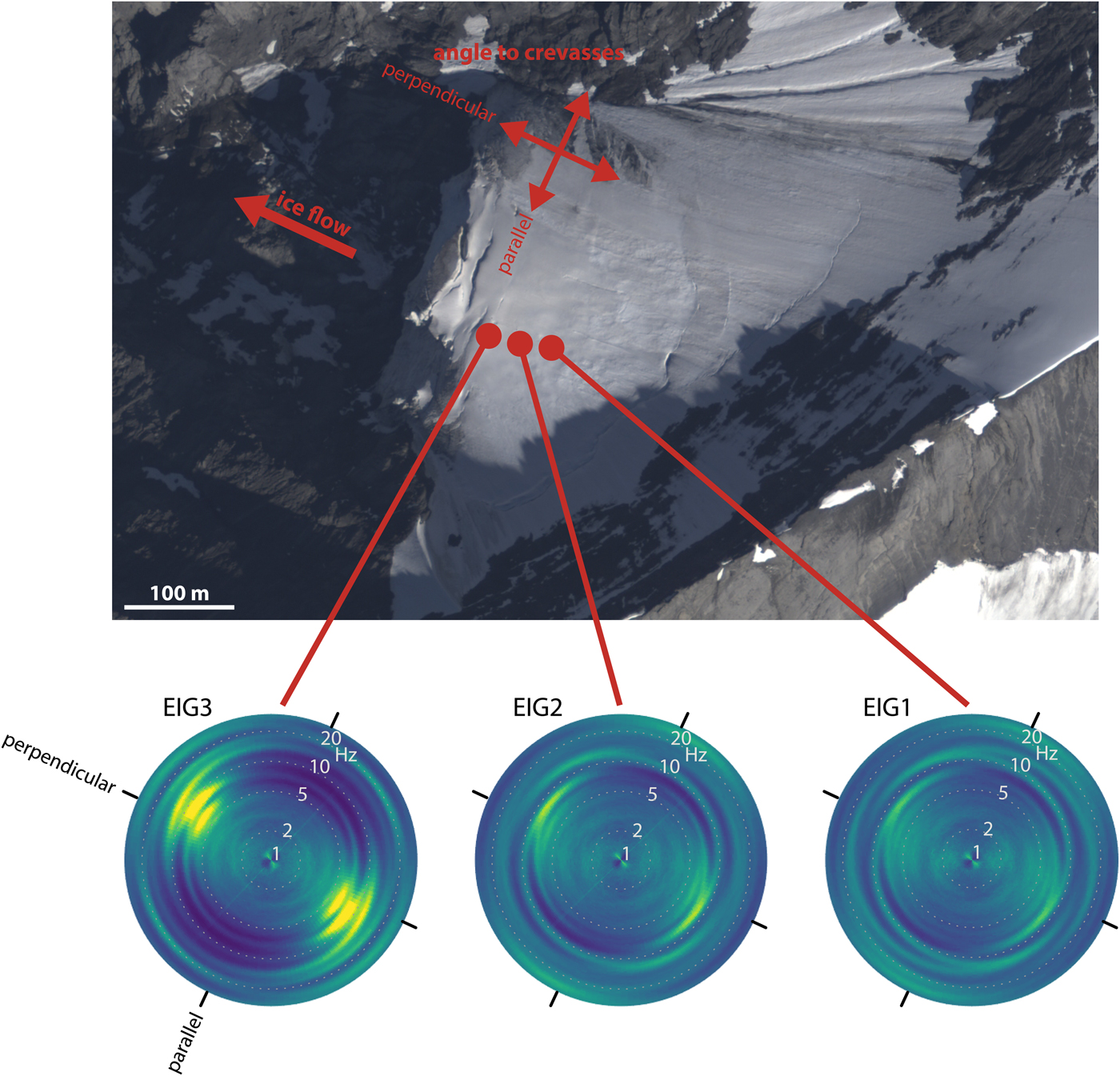
Fig. 7. The polarization as a function of frequency and azimuth at different stations on Eiger-Westflanke. The radial scale denotes the frequency (Hz). Aerial photo: swisstopo flight line 1308201608260940, 26 August 2016.
We further analyze this with the help of Fig. 7, where we plot polarization as a function of azimuth and frequency for three stations. They locate along a line perpendicular to the calving front, with EIG3 being the closest. Just below EIG3, there is a deep crevasse that will most likely be the cause of a future break-off event. Polarization increases toward the ice front: Perpendicular to the crevasses, the peaks at roughly 6.7 and 9.2 Hz are higher closer to the front. The lower frequencies (<3 Hz) as well as the HVSR for components subparallel to the crevasses are not as clearly affected.
The modal analysis using FDD with EIG2 as a reference provides results that are generally difficult to interpret apart from a peak at 9.5 ± 0.3 Hz (Fig. 8a). The associated modal shape (Fig. 8b) exhibits a rigid body translation in the direction of flow. This means that up to this frequency, the vibrations involve the whole structure (respectively the part that is covered by the seismometers). This is however stiffer (higher frequencies) than the expected 1-D-resonance (4.1 Hz, Eqn 1). It should be noted that the spatial coverage of the measurement might not be sufficient to capture the various modes of the system.
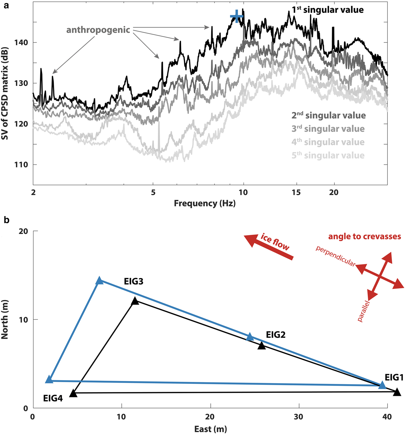
Fig. 8. (a) The singular values of the cross power spectral density (CPSD) matrix of the seismic signal from Eiger-Westflanke. The main observable mode at 9.5 ± 0.3 Hz is highlighted with a cross. Likely anthropogenic monochromatic peaks are marked. (b) Corresponding modal shape (first singular vector at the picked frequency) exhibiting a rigid body translation in the direction of flow (the black triangle is the original array geometry, the blue triangle the deflected array). The amplitude of motion is relative.
For such slender geometry such as an ice wall cut by deep crevasses, in addition to shear deformation, flexural motion can occur. This provides flexibility to the system and therefore shifts the resonance frequencies toward lower values. In this case, the interpretation of the resonance frequency using Eqn 1 may also lead to large biases as shown by Michel and Guéguen (Reference Michel and Guéguen2018).
This leads us to the conclusion that the wavefield of the Eiger-Westflanke is 3-D. The difference to Glacier de la Plaine Morte results from a combination of the overall deeper trough shape and the prominent crevasses. Those crevasses separate individual seracs from each other, and are expected to become progressively deeper toward the calving front (Benn and others, Reference Benn, Hulton and Mottram2007). If the only cause of the 3-D effect was the non-axisymmetric structure, the polarization would not change this strongly within few meters. The crevasses (3-D geometry) however become increasingly deeper even on such a small scale. The wavefield of the stations closer to the front are more strongly affected by the crevasse.
Aletschgletscher - 2-D resonance?
Aletschgletscher is situated in a deep glacially carved valley. Yet, the equivalent shape ratio estimate would place it in the 1-D regime (Fig. 3). In Figure 10, we show an overview over the array on a shaded digital elevation model.
In the mean of the HVSR curves for all stations, there are several local maxima (Fig. 9). The confined peaks in the HVSR at many stations (1.15 and 1.4 Hz) are interpreted as monochromatic non-glacial noise, despite our efforts to avoid such undesired influences as much as possible. Ignoring those, there is a broad but small resonance peak around 1 Hz (Fig. 9). The synthetic ellipticity curves, calculated using Eqn 1 for 400 m ice thickness, reveal that the expected resonance peak has a low amplitude and a slightly lower frequency.
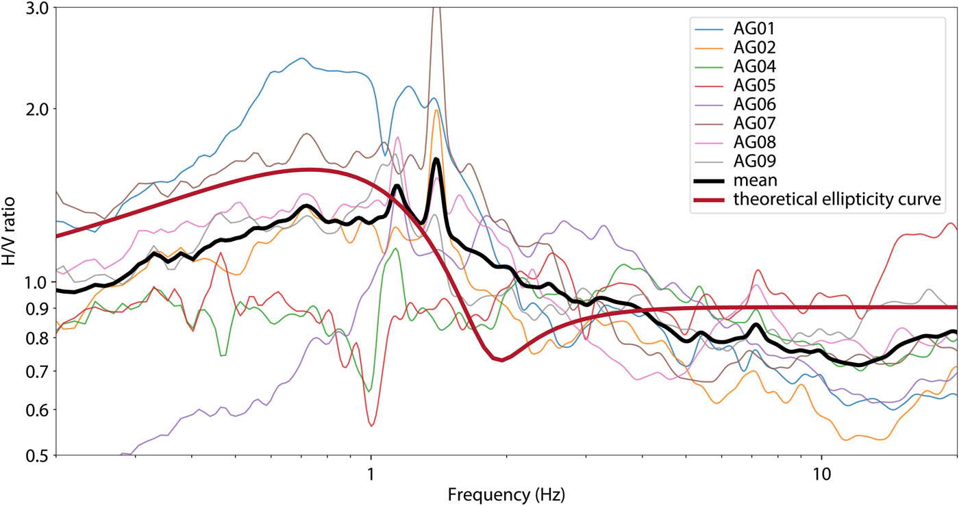
Fig. 9. HVSR of Aletschgletscher with a theoretical ellipticity curve for 400 m ice over bedrock. The overall shape of the curve has some resemblance to the theoretical prediction, but it is influenced also by anthropogenic noise (e.g. the monochromatic peaks at 1.15 and 1.4 Hz).
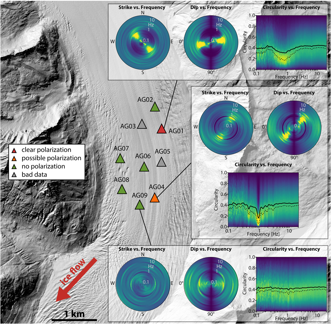
Fig. 10. Time-frequency-dependent polarization analysis (TFPA) of the stations on Aletschgletscher. Most stations do not show a clear polarization, except for AG01, which also shows the most pronounced peak in the HVSR. At AG04, ignoring the monochromatic anthropogenic disturbance, the wavefield also seems to be polarized. None of the other stations shows a polarization. Also, the crevasses seemingly do not affect the wavefield, contrary to Eiger-Westflanke. Polarization plots of stations not shown here can be found in Figure S2. Background image: digital elevation model swissALTI3D (relief), 2016.
The TFPA measurements are also affected by the anthropogenic noise, but do not reveal a clear polarization at the resonance frequency except for one station (station AG01), and a potential polarization at a second station (AG04, ignoring the monochromatic signal at 1 Hz, Fig. 10). Additionally, we do not observe a pattern consistent throughout the array as expected for a 2-D resonance case (Fig. 1, Ermert and others, Reference Ermert, Poggi, Burjánek and Fäh2014), nor a dominant influence of the crevasses. Therefore, we suspect that Aletschgletscher can be approximated as a 1-D structure.
Picotti and others (Reference Picotti, Francese, Giorgi, Pettenati and Carcione2017) note that at their field site, several kilometers upstream of our site, the glacier thickness is comparable with the valley half-width, invalidating the 1-D approximation. At our site, the valley is narrower but also the glacier is thinner. The geologic situation and therefore the impedance contrast between ice and bedrock is similar for both sites (swisstopo, 2005). One difference is the anthropogenic noise, which is intense at our site during our measurements, but less visible in the HVSR of Picotti and others (Reference Picotti, Francese, Giorgi, Pettenati and Carcione2017) measured 2 years earlier (Fig. 11 therein). However, it should be noted that their smoothing constant (Konno and Ohmachi, Reference Konno and Ohmachi1998) is 25, which results in a broader peak compared with the value of 80 that we use, which could potentially blur monochromatic peaks.
DISCUSSION
The thicknesses of several glaciers and ice sheets have recently been estimated using HVSR. However, using this method blindly on all available data can lead to biased results. For example, the popular geopsy software package (Wathelet, Reference Wathelet2008) allows only the inversion of the classical properties of surface waves (dispersion curves, ellipticity of Rayleigh waves) into structural models. Using the HVSR curve in this context, one assumes that the wavefield is dominated by Rayleigh waves, which is not always the case. Even if it is dominated by Rayleigh waves, or if another method such as the DFA is used, the inversion of HVSR is still non-unique. With enough additional data, it can lead to reasonable glacier thickness estimates, when the limitations of the method are known (Picotti and others, Reference Picotti, Francese, Giorgi, Pettenati and Carcione2017). Yan and others (Reference Yan2018) used an algorithm based on the DFA (García-Jerez and others, Reference García-Jerez, Pina-Flores, Sánchez-Sesma, Luzón and Perton2016) to obtain thicknesses of the Antarctic Ice Sheet. As the structure is close to 1-D, they were successful at most sites and retrieved thicknesses comparable to Bedmap2 (Fretwell and others, Reference Fretwell2013). They encountered difficulties at stations with suspected more complicated subglacial environments. In such cases, a 2-D/3-D geometry for the inversion would be necessary (Roten and Fäh, Reference Roten and Fäh2007; Ermert and others, Reference Ermert, Poggi, Burjánek and Fäh2014). Nevertheless, we still find HVSR useful to estimate bedrock depth in combination with other methods. It could be of use, for example, on debris-covered glaciers, where it is inconvenient to deploy methods such as radio-echo sounding.
At Eiger-Westflanke, the observed directionality of the wavefield is similar to unstable rock slopes (e.g. Burjánek and others, Reference Burjánek, Gassner-Stamm, Poggi, Moore and Fäh2010; Kleinbrod and others, Reference Kleinbrod, Burjánek and Fäh2017a): At the resonant frequencies, the ground motion is locally amplified in the direction parallel to the dominant deformation, i.e. perpendicular to open fractures. This information can be used to delineate stable from unstable rock slope parts, therefore allowing a volume estimation of the unstable part (Burjánek and others, Reference Burjánek, Moore, Molina and Fäh2012). Changes in the polarization or resonance frequencies can be used for monitoring unstable rock slopes and columns (Lévy and others, Reference Lévy, Baillet, Jongmans, Mourot and Hantz2010; Burjánek and others, Reference Burjánek, Gischig, Moore and Fäh2017). Applied to avalanching glaciers, this method could complement existing forecasting techniques (Faillettaz and others, Reference Faillettaz, Funk and Vincent2015). Nevertheless, numerical modeling will likely be necessary to improve our understanding of such complex systems, and to reveal the differences and similarities between unstable rock slopes and avalanching glaciers.
The non-1-D resonance frequencies observed here may reveal information about crevasse depth. In the absence of independent measurements, this remains hypothetical. An experiment to determine the relation between crevasse depth and resonance frequency would shed more light on this issue. Such a relation would be highly beneficial, as conventional crevasse depth measurements with plumb line systems are cumbersome and unsuitable for monitoring (Mottram and Benn, Reference Mottram and Benn2009). Yet, crevasse depth is critical to accurately model the calving process and therefore ultimately mass loss through calving (e.g. Benn and others, Reference Benn, Hulton and Mottram2007). This could be interesting for monitoring unstable glaciers (Preiswerk and others, Reference Preiswerk2016), with the advantage being that only a single station is necessary.
CONCLUSIONS
We have analyzed the ambient wavefield of a plateau glacier, a highly crevassed avalanching glacier, and a large valley tongue. We showed that geometry of the glacier bed, crevasses, as well as anthropogenic noise have a strong influence of the wavefield. Using HVSR with a 1-D assumption to estimate ice thickness was justified for Glacier de la Plaine Morte (plateau glacier). Due to low velocity contrast between ice and bedrock, the peaks in the HVSR are small in our observation as well as in the theoretical prediction. Thickness estimation using HVSR works to a lesser extent also for Aletschgletscher (valley glacier), where the monochromatic peaks of anthropogenic origin have a higher amplitude than the resonance peak.
On the avalanching glacier at Eiger-Westflanke, the deep trough shape and the dominant crevasses lead to 3-D effects and 2-D/3-D eigenvibrations, invalidating the 1-D assumption of HVSR. FDD of the wavefield shows that the structure is vibrating as a rigid body in the direction of ice flow. Finally, polarization analysis at Eiger-Westflanke revealed that the dominant direction of ground motion is perpendicular to the crevasses. The frequency of the polarization might be related to the crevasse depth, which would be a key parameter for modeling avalanching and calving glacier fronts.
SUPPLEMENTARY MATERIAL
The supplementary material for this article can be found at https://doi.org/10.1017/aog.2018.27.
ACKNOWLEDGMENTS
We thank the editor, Douglas R. MacAyeal, and two anonymous referees for their expeditious and constructive reviews. The Swiss National Science Foundation financed the salaries of LEP and FW and part of the instrument deployment (GlaHMSeis Project PP00P2_157551). We would like to acknowledge logistical support from Fritz Brawand and the Jungfraubahnen as well as Remontées Mécaniques de Crans-Montana (CMA). We are grateful to Jan Burjánek, Martin Funk, Mauro Häusler, Agostiny Lontsi, Martin Lüthi and Samuel Weber for valuable discussions, as well as to our technicians Pascal Graf and Robin Hansemann, and to everyone who helped in the field.
LEP and FW designed the experiments and collected the data. LEP analyzed the data and created the plots with the help of CM. LEP, CM, FW and DF interpreted the data. LEP wrote the manuscript with significant input and critical reviews by CM, FW and DF.


 Open access