


Introduction
Meltwater from glaciers in Alaska has made a substantial contribution to sea-level rise in the past decades (Reference ArendtArendt and others, 2006; Reference VanLooy, Forster and FordVanLooy and others, 2006; Reference Berthier, Schiefer, Clarke, Menounos and RémyBerthier and others, 2010) and will likely continue to do so in the future (Reference Radić and HockRadić and Hock, 2011; Reference Marzeion, Jarosch and HoferMarzeion and others, 2012; Reference GardnerGardner and others, 2013), assuming further increases in temperature. Reference GardnerGardner and others (2013) determined the sea-level rise contribution of all glaciers globally for 2003–09 using a combination of satellite-based methods (gravimetry and elevation changes) and field-based measurements of glacier mass balance. For the purpose of that study, the sparsely available field data (Reference Zemp, Hoelzle and HaeberliZemp and others, 2009) were extrapolated to entire mountain ranges using an inverse distance-weighted (IDW) scheme adopted from Reference CogleyCogley (2009). The high uncertainty of this method is well known, as mass budgets of individual glaciers in the same mountain range can vary strongly (Reference Kuhn, Markl, Kaser, Nickus, Obleitner and SchneiderKuhn and others, 1985; Reference HussHuss, 2012). However, the measured glaciers were found to have more negative mass budgets than the regional averages obtained by satellite methods, thus introducing a bias towards an overestimation of their sea-level rise contribution (Reference GardnerGardner and others, 2013). Determining the representativeness of the measured mass-balance glaciers for the mass changes of an entire region is thus still a key issue for global-scale extrapolations (Reference Kaser, Cogley, Dyurgerov, Meier and OhmuraKaser and others, 2006). On the other hand, in regions such as the European Alps, with a wealth of calibration data and repeat digital elevation models (DEMs), such an assessment is readily feasible (Reference HussHuss, 2012).
In Alaska, only two glaciers (Gulkana and Wolverine) have long-term records of direct mass-balance measurements (Reference Van Beusekom, O’Neel, March, Sass and CoxVan Beusekom and others, 2010), and DEMs covering large regions are only available for two points in time. These DEMs were used by Reference Berthier, Schiefer, Clarke, Menounos and RémyBerthier and others (2010) to calculate overall mass budgets and sea-level-rise contributions for all glaciers in Alaska over a 50 year time period. That study revealed a high spatial variability of elevation changes and a pronounced thinning of the often low-lying tongues of large valley glaciers. With the recently published glacier inventory for western Alaska (Reference Le Bris, Paul, Frey and BolchLe Bris and others, 2011), drainage divides of individual glaciers can be digitally intersected with the elevation change raster data and glacier-specific values can be calculated. This also allows exclusion of specific glaciers from the averaging process (e.g. when more than 20% of the area is covered by data voids in the DEMs) and separating the changes for different types of glaciers (e.g. land-terminating vs tidewater).
By comparing the volume changes derived for the two benchmark glaciers to the overall mean of a selected sample (e.g. all land-terminating glaciers derived by differences of DEMs), a factor can be obtained that allows upscaling of their changes measured for the entire region (Reference Paul and HaeberliPaul and Haeberli, 2008). Of course, such factors only hold for the investigated period and for multi-year (e.g. pentadal) averages of volume changes (Reference CogleyCogley, 2009). But the method is independent of measured mass budgets, thus avoiding problems with an unknown snow/firn/ice density (Reference HussHuss, 2013) and the challenges of comparing geodetic volume changes to cumulative glacier-wide extrapolations of field measurements of point mass balances (Reference FischerFischer, 2011; Reference ZempZemp and others, 2013). The method should also provide more accurate results for an entire region than IDW interpolation. A direct comparison of the geodetic with the glaciologically derived cumulative mass budget for Gulkana Glacier is presented by Reference Cox and MarchCox and March (2004).
In this study we calculate mean elevation changes (i.e. normalized with the area) for a sample of 3180 glaciers in western Alaska to determine the representativeness of the two glaciers with long-term mass-balance measurements (Gulkana and Wolverine) for the entire region. Special emphasis is given to the different possibilities of calculating mean values for the entire region (arithmetic or area-weighted) and the treatment of DEM artefacts when deriving glacier-specific mean values.
Study Region, Data Sources and Processing
Study region
The study region is located in the western Alaska Range, including the Tordrillo, Chigmit, Katmai and Chugach Mountains as well as the Kenai Peninsula (Fig. 1). All types of glaciers are present in this region, from cirques, mountain and valley glaciers to ice-clad volcanoes and ice caps. The glacier inventory of western Alaska compiled by Reference Le Bris, Paul, Frey and BolchLe Bris and others (2011) includes more than 8800 glaciers >0.02 km2 covering a total area of 16 250 km2, which is about 19% of the glacierized area of Alaska according to Reference PfefferPfeffer and others (2014). Only 0.4% of the glaciers are >100 km2 but they account for 47% of the total area. Only a few glaciers (36) in the study region are calving in lakes (lacustrine) or the ocean (tidewater), but they are comparatively large (e.g. Columbia Glacier, with an area of 945 km2). Glaciers stretch from sea level up to 4000 m a.s.l. and the observed trend of mean elevations implies a significant decrease of precipitation from the coast towards the interior of Alaska (Le Bris and others, 2011).

Fig. 1. Location map showing the glaciers (blue) with a hillshade of the NED DEM in the background. Inset shows the study region in Alaska.
Datasets and pre-processing
The glacier outlines used here are a subset of the Digital Line-Graph (DLG) dataset for Alaska compiled by the US Geological Survey (USGS) by either manual or automated digitizing based on large-scale 7.5 min topographic quadrangle maps (1: 25 000 and 1: 63 360 scales for Alaska). For quality control of the DLG outlines we compared them with the Digital Raster Graph (DRG) dataset, which is a high-resolution scan of published paper maps that have a date (topomaps.usgs.gov/drg). This overlay revealed a systematic planimetric shift between the DLG and the DRG, which is explained on the aforementioned DRG website. The observed outline mismatches (especially in the ablation region of glaciers) were adjusted manually for a subset of the DLG glacier outlines (350 glaciers) according to the DRG maps (Fig. 2) for an evaluation of the impact of non-adjusted extents on glacier mass balance (e.g. Reference PaulPaul, 2010; Reference HussHuss and others, 2012).

Fig. 2. (a) Elevation change for uncorrected DLG vs corrected DLG glacier outlines. (b) Red arrows show the glacier extents visible on the topographic map (DRG).
The USGS National Elevation Dataset (NED) is a DEM derived from contours as given on topographic maps from the 1950s (Reference GeschGesch, 2007) and is used as the base for calculating elevation changes. For Alaska, the NED DEM is available at 2 arcsec postings (~60 m). The absolute vertical accuracy of the quadrangle-based USGS 7.5 min DEMs is reported to be 7 m, but due to poor contrast in the accumulation areas accuracy can be much lower (e.g. Aðalgeirsdóttir and others (1998) and Reference Arendt, Echelmeyer, Harrison, Lingle and ValentineArendt and others (2002) assumed a 45 m uncertainty in this region). The product was downloaded through the USGS Seamless Server (seamless.usgs.gov).
The elevation changes from 1950 to 2006 (Δh/Δt raster maps) used here to determine glacier-specific values were derived by Reference Berthier, Schiefer, Clarke, Menounos and RémyBerthier and others (2010) and are based on the subtraction of two DEMs. The older DEM is the USGS NED described above and the more recent DEM was derived from the high-resolution stereoscopic (HRS) sensor on board SPOT 5 (Satellite Pour l’Observation de la Terre) (Reference Bouillon, Bernard, Gigord, Orsoni, Rudowski and BaudoinBouillon and others, 2006) and created within the framework of the International Polar Year (IPY) project SPIRIT (Spot 5 stereoscopic survey of Polar Ice: Reference Images and Topographies, Université de Toulouse) described by Reference Korona, Berthier, Bernard, Rémy and ThouvenotKorona and others (2009). This DEM has a 40 m cell size, a horizontal confidence region of 30 m, and a vertical confidence region between –5.5 and +3.5 m (compared with the Ice, Cloud and land Elevation Satellite (ICESat)). Nonetheless, an elevation uncertainty of ±10 m is assumed over the entire study area.
To determine elevation changes for the two benchmark glaciers, which had too many data voids in the SPIRIT DEM, we also used the Advanced Spaceborne Thermal Emission and Reflection Radiometer (ASTER) global DEM (GDEM2) compiled from all available stereo-pair images in the ASTER archive acquired between 2000 and 2011. The GDEM2 has a spatial resolution of 30 m and a vertical accuracy of about 7–14 m (standard deviation) (ASTER Validation Team, 2009; Reference Fujisada, Urai and IwasakiFujisada and others, 2012).
Individual glacier extents were derived by digital intersection with drainage divides derived from hydrological computations (watershed analysis) using the NED DEM and GIS tools following the approach of Reference Bolch, Menounos and WheateBolch and others (2010). Hillshade images were created for all DEMs to check quality and artefacts.
Methods
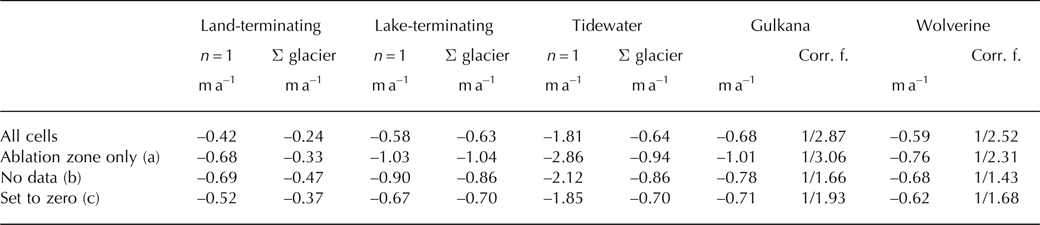
As a first step of the statistical analysis, glaciers <0.05 km2 or with >20% of their area covered by data voids are excluded. In a second step three types of glaciers are distinguished (i.e. marked in the attribute table): land-terminating, lake-terminating and tidewater glaciers. Outside of data voids, DEM artefacts can occur in areas of low contrast (e.g. covered by snow and shaded slopes) that might result in artificial positive elevation changes (i.e. mass gain). To determine the influence of these regions on the mean values, we calculated mean elevation changes for each glacier by three different methods: (a) for the ablation areas only (regions below the mean elevation as a rough proxy for the long-term equilibrium-line altitude (ELA)); (b) by setting all positive elevation changes to ‘no data’; and (c) by setting them to 0 (Table 1). The glacier-specific mean elevation changes for the three samples (a), (b) and (c) were then averaged for the entire region in two statistically different ways: (1) one mean value for the entire study region to determine the overall changes (area-weighted); and (2) the arithmetic mean of all individual mean elevation changes.
Table 1. Mean elevation change as a function of glacier type calculated by two methods of averaging: n = 1 uses one mean value for the entire study region; Σ glacier uses the arithmetic mean of individual mean elevation changes. Rows 2–4 reflect different ways of calculating the influence of potential DEM artefacts. Corr. f. is the multiplicative correction factor (required to obtain the mean value of the land-terminating glaciers)
Owing to the different cell sizes of the DEMs subtracted (30, 40 and 60 m), resampling effects and elevation-dependent biases might occur in the difference grid (Reference Paul and HaeberliPaul and Haeberli, 2008); they can be corrected by considering the maximum terrain curvature (Reference Gardelle, Berthier and ArnaudGardelle and others, 2012). However, we did not find any systematic elevation changes for terrain outside of glaciers (Fig. 3) and thus have not corrected for them. This lack of systematic change is likely due to the very similar level of detail in all three DEMs as seen in a visual comparison of hillshades.

Fig. 3. Elevation differences between NED and GDEM2 for flat terrain off glaciers (with slopes <5°).
To assess the usefulness of the GDEM2 for determining elevation changes, we computed mean elevation changes between the GDEM2 and the NED DEM (Fig. 3) and compared them with the values derived from the dataset of Reference Berthier, Schiefer, Clarke, Menounos and RémyBerthier and others (2010) using SPOT data. Co-registration between the NED DEM and the GDEM2 was achieved following the method developed by Nuth and Kääb (2011), which uses terrain aspect to quantify the offset values with an iterative approach.
Owing to data voids covering >20% of the area in the Δh/Δt raster maps for the two benchmark glaciers (Gulkana and Wolverine), we had to determine elevation changes specifically for these glaciers by differencing the NED DEM and the GDEM2 (a useful DEM derived from only one ASTER scene was not available). To determine if the multi-year composite GDEM2 is suitable for this purpose, we compared glacier-specific elevation changes derived with the GDEM2 to those derived from the SPOT DEM for other glaciers. Mean elevation changes for each glacier were calculated using zone statistics in the GIS software and divided by the number of years between the two DEMs to obtain rates of elevation change. Topographic maps were acquired over a 7 year period so that using the mean value of the epoch as a reference date results in an uncertainty of ±3.5 years, which translates into an elevation uncertainty of ±2.5 m according to Arendt and others (2006) and Reference Berthier, Schiefer, Clarke, Menounos and RémyBerthier and others (2010).
Results
Elevation changes
In total, elevation changes were calculated for ~3180 glaciers. The mean change (area-weighted) for the entire study region is –0.67 ± 0.76 m a–1, with a mean value of –0.42 ± 0.35 m a–1 for land-terminating glaciers, –0.58 ± 0.87 m a–1 for lake-terminating glaciers, and 1.81 ± 2.24 m a–1 for tidewater glaciers including Columbia Glacier and –0.60 ± 0.90 m a–1 excluding it. The extreme loss of Columbia Glacier (–2.8 m a–1) has a strong impact on the area-weighted mean thinning rate.
Colour-coded glacier-specific mean values of elevation change for three subsections of the study region are shown in Figure 4. The high variability in the changes is evident in Figure 4, even for glaciers originating at the same mountain ridge. A more detailed analysis revealed that mean elevation changes are weakly correlated with glacier size, but not with mean slope, exposition or mean elevation. Several small to medium-sized glaciers experienced a net increase in elevation when the differences were used as calculated. In some cases these increases might be related to artefacts in the DEM that have an increasing impact on the mean value towards smaller glaciers.

Fig. 4. Examples of mean elevation changes in (a) Tordrillo and Chigmit Mountains, (b) Chugach Mountains and (c) Kenai Peninsula. White dots indicate lake-terminating and tidewater glaciers. White glaciers represent those with >20% data voids. (d) Insets show the location of the mountain ranges in Alaska.
Such artefacts are also visible in Figure 5, illustrating the spatial distribution of elevation changes on a gridcell level. Apart from Matanuska Glacier (D), all glaciers experienced moderate to strong elevation loss in their lower parts, largely independent of their geographic location. For Gulkana (B), Wolverine (E) and in a less pronounced way also for Trimble Glacier (F), surface lowering also occurred in the accumulation area. Positive elevation changes >0.5 m a–1 are mostly located towards the glacier boundary and at steep slopes. They might thus represent DEM artefacts or result from the different DEM cell sizes compared. Values between 0 and +0.5 m a–1 are within the uncertainty range of the DEMs and can be real or not. The gain/loss dipole in the accumulation region of Wolverine Glacier could also be an artefact of local DEM quality (e.g. Reference KobletKoblet and others, 2010).
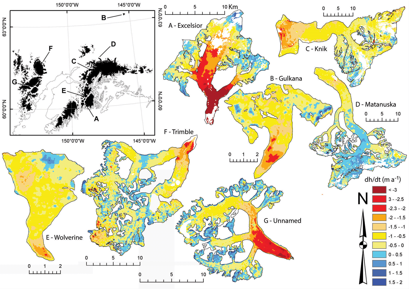
Fig. 5. Elevation changes for seven glaciers. Glacier outlines are from the DLG dataset. White areas indicate no data. Inset shows the location of the seven glaciers. A: Excelsior Glacier; B: Gulkana Glacier; C: Knik Glacier; D: Matanuska Glacier; E: Wolverine Glacier; F: Trimble Glacier; G: unnamed glacier in the Chigmit Mountains.
The impact of the different methods for excluding potential artefacts (positive changes) from calculations of mean values are listed in Table 1 for the three types of glacier and two types of averaging. In general, the mean changes are more negative for the area-weighted calculation (land-terminating and tidewater), but for lake-terminating glaciers they are very similar. Regarding the different methods for considering positive changes, mean changes are (as expected) in general more negative when only the ablation area (below the mean elevation) is considered. However, for land-terminating glaciers the replacement of positive values with no data gives even more negative changes, indicating that substantial surface lowering also took place above the mean elevation. For some glaciers (e.g. C and F in Fig. 5) artefacts (or general DEM errors) might also be related to negative changes (red spots in the accumulation region). These have not been considered for correction here as they occur much less frequently, thus having a small impact on the overall mean (i.e. real changes would be slightly less negative); however, when analysing individual glaciers there might be a need to correct for these as well.
Figure 6 illustrates the elevation changes averaged over 50 m elevation bins for the ten largest land-terminating glaciers and the two benchmark glaciers (Gulkana and Wolverine). For all glaciers the strongest losses occurred at their lowest parts between 250 and 750 m a.s.l. Between 1000 and 2000 m a.s.l., changes are similar for the largest glaciers, apart from Gulkana Glacier, which over large parts of its elevation range has much stronger losses than all other glaciers at this elevation. Towards higher elevations several glaciers show thickening (e.g. Capps Glacier with up to 0.5 m a–1), some show little change and some show increasing loss with altitude, as mentioned above. However, some of these changes are likely related to artefacts, implying that the values should not be over-interpreted.
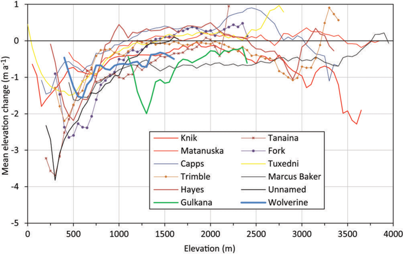
Fig. 6. Mean elevation changes in 50 m elevation bins for the ten largest glaciers. Gulkana (17.9 km2) and Wolverine (17.17 km2) benchmark glaciers are also included.
Further investigations on the dependence of elevation changes on other glacier parameters (e.g. size, mean elevation, elevation range, slope and distance from the ocean) did not reveal any significant correlations (Fig. 7), indicating local highly variable climatic regimes and glacier responses that also depend on the variable geometry of each glacier (i.e. its hypsometry).
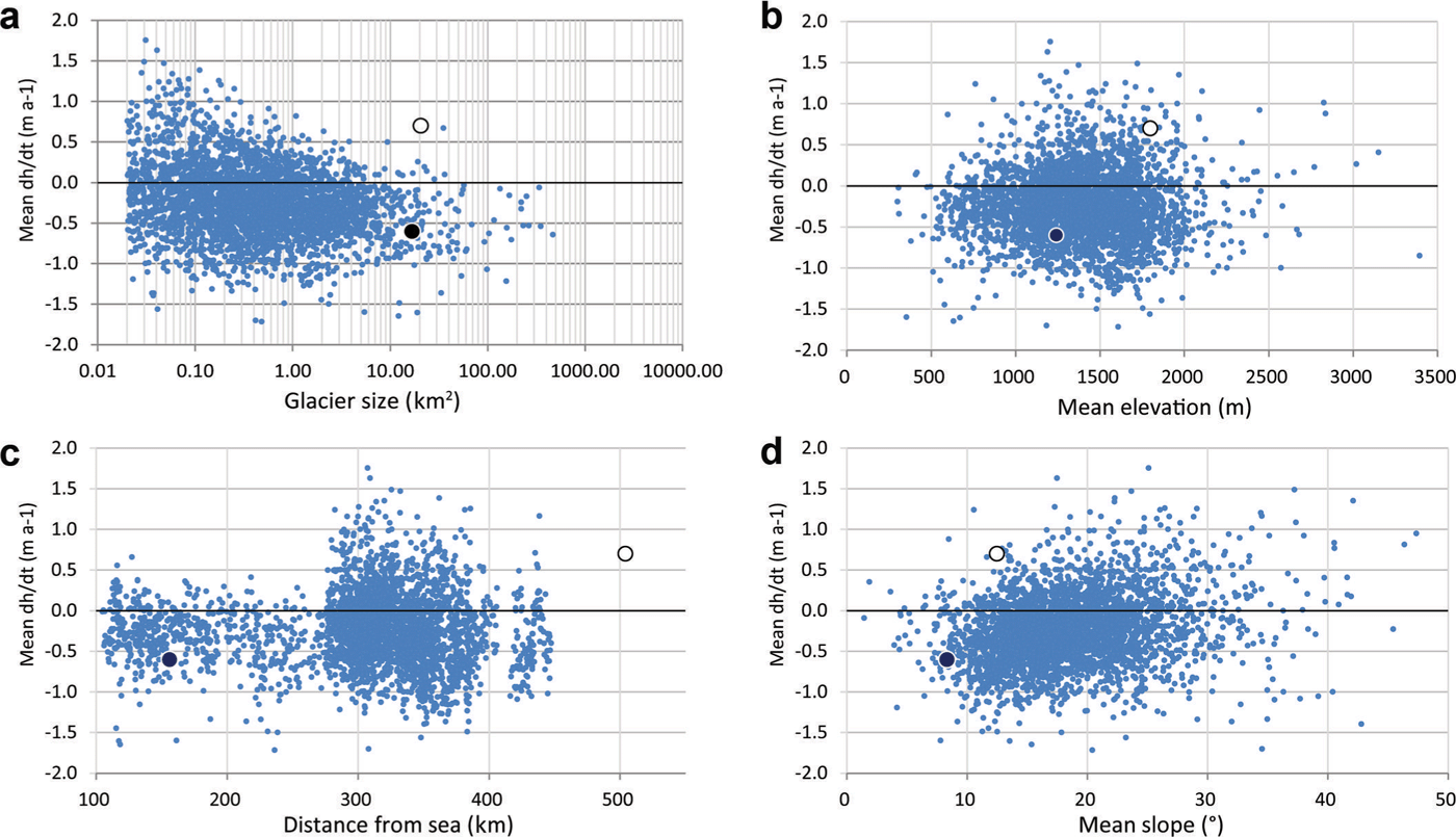
Fig. 7. Elevation change vs other glacier parameters: (a) glacier size, (b) mean elevation, (c) distance from the ocean and (d) elevation range. Black and white dots represent Wolverine and Gulkana Glaciers, respectively.
Correction factors
Whether one prefers to compare the mean values of Gulkana and Wolverine Glaciers (–0.7 and –0.6 m a–1) with the values from either the arithmetic or the area-weighted averaging of the respective larger sample is a matter of purpose. To determine their representativeness, we compare them with the arithmetic means, revealing that their values are much more negative (factor of 2–3) than for the other land-terminating glaciers (–0.24 m a–1). In fact, their values are much closer to the other two types of glacier (in particular lake-terminating), and also when considering the three ways of excluding artefacts (Table 1).
In other words, extrapolating the changes for these two glaciers would overestimate the losses of other land-terminating glaciers by a factor of 2.5 (for Wolverine) and 2.9 (for Gulkana), consistent with the results of Reference GardnerGardner and others (2013) who concluded that measured glaciers introduce a bias when simply extrapolated to their surrounding regions. On the other hand, their mean change is very close to the mean of the entire region (including the calving glaciers) and they can thus be considered representative for the entire region investigated here. When the exceptionally strong elevation loss of Columbia Glacier is excluded, the agreement is less good, and uncorrected extrapolation would yield mass budgets ~30% too negative. However, when considering the standard deviations, the mean elevation change rates for the three glacier types are not significantly different and should thus be interpreted prudently. It also should be emphasized that the above factors are only valid for the time period covered by the two DEMs and might be different for other periods.
Accuracy of the GDEM2
Data voids were too large in the SPIRIT DEM over Gulkana and Wolverine Glaciers, so we had to use the GDEM2 to calculate elevation changes with the NED DEM. As the GDEM2 is a merged multitemporal product, it is necessary to determine whether it can be used as an alternative to the product derived from SPOT. For this purpose we first determined the elevation differences between the GDEM2 and the SRTM DEM for weakly inclined (slopes <5°) and stable terrain off-glaciers for a region south of Wolverine Glacier (Fig. 3). The mean difference is –6.13 ± 12.2 m when masking all glaciers and the ocean. At first glance this is a high value, but as shown clearly in Figure 3 it is mostly due to artefacts of the GDEM2. There are issues with regions of low or confusing contrast (e.g. from gravel plains that are related to the three well-confined regions in the middle and upper right of Fig. 3), as well as along boundaries of the merged ASTER tracks (Fig. 3, upper left). Overall, this comparison revealed the well-known problems of the GDEM2, but was not conclusive about its accuracy. By visually excluding the artefact regions, most elevation differences are in the ±5m range (green and cyan), pointing to a mean difference much closer to zero and thus acceptable for the purpose of this study. However, as this result is somewhat unsatisfactory, we also compared mean elevation changes derived with both DEM pairs (NED/GDEM2 and NED/SPOT) for a sample of 2940 glaciers (Fig. 8). In general, there are no size-dependent trends of the differences and the scatter increases towards smaller glaciers. Table 2 lists size-class-specific mean values and standard deviations. For the 10–20 km2 size class (encompassing 72 glaciers) of Gulkana (17.17 km2) and Wolverine (17.8 km2) Glaciers, the standard deviation is only 0.12 m a–1 and thus within acceptable limits of such measurements (Reference ZempZemp and others, 2013). The NED/GDEM2-derived values for the two glaciers were finally bias-corrected with the mean difference to the NED/SPOT-derived values of this size class (0.09 m a–1).
Table 2. Differences in elevation changes over glaciers (mean and standard deviation) derived from two combinations of DEMs (NED/SPOT and NED/GDEM2) for 2940 glaciers of different sizes (see Fig. 8 for individual differences) sorted for size class. Note that, for the 100–500 km2 size class, one outlier (Excelsior Glacier) was removed
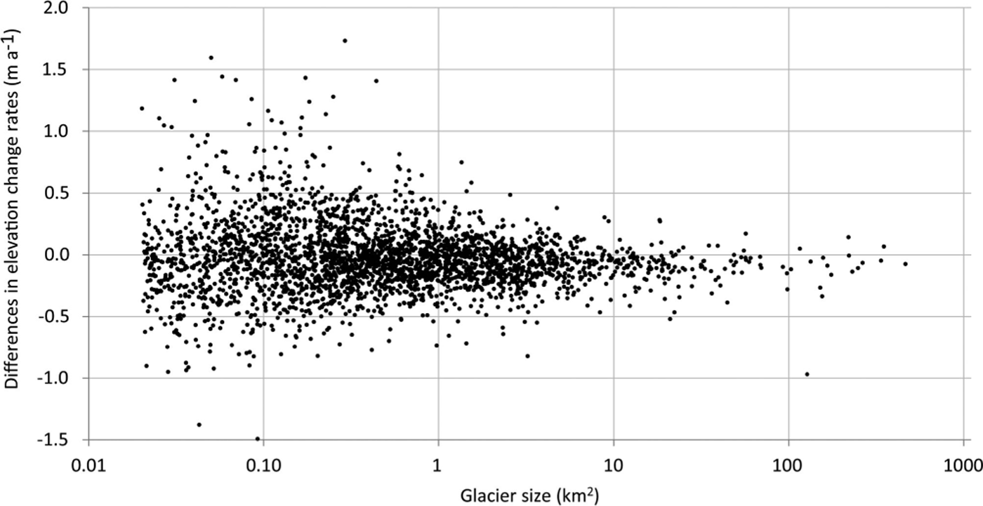
Fig. 8. Comparison of the mean elevation changes derived with both DEM pairs (NED/GDEM2 and NED/SPOT) for a sample of 2940 glaciers.
Discussion
Elevation changes
The general tendency of glacier volume loss found here is in line with earlier studies in this region (Arendt and others, 2002; Reference Berthier, Schiefer, Clarke, Menounos and RémyBerthier and others, 2010), but is now also available as a mean value for individual glaciers. This allowed us to exclude lake-terminating and tidewater glaciers from the sample and to determine how the mean elevation changes of the two benchmark glaciers compare to the means of all other land-terminating glaciers. The two benchmark glaciers had about two to three times more negative changes, thus confirming the findings of Reference Fountain, Hoffman, Granshaw and RiedelFountain and others (2009) and Reference GardnerGardner and others (2013) that the glaciers selected for mass-balance measurements might have a negative bias. Compared with the other glaciers in the region, the benchmark glaciers might be smaller or larger, located at a different elevation, too flat and/or less shaded. However, this changes when calving glaciers are also considered, as they have similar loss rates to the two benchmark glaciers (about –0.6 m a–1). Hence, for determination of the sea-level contribution of the entire region their specific mass budgets can indeed be considered representative and thus used for an upscaling over the region and time period investigated herein (Reference Kaser, Cogley, Dyurgerov, Meier and OhmuraKaser and others, 2006).
This is similar for the Alps, where some of the measured glaciers also had much more negative mass balances over a 15 year period than the other glaciers in their size class (Reference Paul and HaeberliPaul and Haeberli, 2008; Reference HussHuss, 2012). However, they also represent quite well the mean over the entire region as the (unmeasured) largest glaciers contribute much more strongly to the total volume change, as has been revealed from DEM differencing. Thus, despite their different characteristics, the measured glaciers seem to be suitable for upscaling of their mass budgets to the entire region, at least over the time period analysed here.
The extreme loss (–2.8 m a–1) and large size (nearly 1000 km2) of Columbia Glacier are both exceptional characteristics. The changes of this glacier have a strong impact on the overall mean when an area-weighted mean value is determined. However, as the elevation change of tidewater glaciers is also influenced by glacier dynamics rather than climate change (Reference Pfeffer and HarperPfeffer and others, 2008), they should be excluded from the sample when climate change impacts are analysed. In this case the surface elevation loss is also different from the sea-level equivalent volume loss, as the loss of ice below sea level is not measured (Reference McNabbMcNabb and others, 2012). The ice volume lost below sea level will be replaced by ocean water with a 10% higher density, thus lowering sea level (Reference Haeberli and LinsbauerHaeberli and Linsbauer, 2013).
Uncertainties
Several uncertainties influence the quality of our results, including: (1) the artefacts in the DEMs; (2) the partially updated glacier extents in the DLG; (3) the use of the GDEM2 instead of the SPOT DEM for the two benchmark glaciers; and (4) uncorrected biases (e.g. due to different DEM resolutions). As we have already discussed points (3) and (4), some comments on points (1) and (2) have to be made.
To be reliable, the overall elevation changes should be larger than the accuracy of the two DEMs. For most glaciers this is true in the ablation area, but less so in the accumulation area. Elevation increases can be real in a very maritime climate, such as coastal Alaska or Norway (Reference Andreassen, Elvehøy, Kjøllmoen, Engeset and HaakensenAndreassen and others, 2005), but they can also be artefacts, in particular when the increase occurs on steep slopes or over shaded or snow-covered terrain with reduced optical contrast (see Fig. 5), the regions typical of poor performance of optical DEMs (e.g. Reference Frey and PaulFrey and Paul, 2012; Reference Gardelle, Berthier, Arnaud and KääbGardelle and others, 2013). When it is not possible to identify these artefacts, setting positive elevation changes to no data may be the best way of excluding potentially wrong values from the analysis. Setting these positive values simply to zero might already introduce a bias, but, as the mean values show (Table 1), the differences between the two methods of calculation are small.
To determine the influence of (2), we corrected the outlines of 350 glaciers from the DLG according to the DRG and compared the mean elevation changes for the corrected and uncorrected extents (Fig. 2). This comparison revealed larger (non-systematic) deviations for only five glaciers, so that in the mean over the entire sample the influence of the missing correction on the calculated change rates is small. After the five outliers are removed, the correlation coefficient and standard deviation are 0.99 and 0.35 m a–1, respectively.
When the overall changes are dominated by a few glaciers, arithmetic averaging does indeed give a different mean value than that resulting from an area-weighted calculation. While the latter should be used when calculating the sea-level contribution (Reference Berthier, Schiefer, Clarke, Menounos and RémyBerthier and others, 2010), the arithmetic mean fits better to the mean values of the direct measurements, as they are also arithmetically averaged.
Conclusions
We have calculated mean elevation changes for 3180 glaciers in western Alaska from two DEMs acquired ~50 years apart to determine the representativeness of Gulkana and Wolverine Glaciers for the mean elevation changes of the entire region. We excluded glaciers with extents >20% covered by data voids and distinguished three types of glacier, four methods to handle possible artefacts, and two methods for statistical averaging of the overall changes. For the two benchmark glaciers we had to use another DEM (GDEM2 instead of SPOT), so we also determined the impact on the derived change values of using this alternative DEM.
Rates of elevation change are –0.63 ± 0.40 m a–1 for both lake-terminating and tidewater glaciers and –0.24 ± 0.44 m a–1 for land-terminating glaciers. Thus, simple extrapolation of the mean elevation changes for Gulkana and Wolverine Glaciers (–0.7 and –0.6 m a–1) would strongly overestimate the contribution from all other land-terminating glaciers, and correction factors of 1/2.5 and 1/2.9, respectively, would be required. However, these two glaciers represent quite well the mean value for other glacier types and the overall changes, at least when Columbia Glacier is part of the sample. Otherwise a 30% overestimation of mass loss would result. The simple extrapolation of the measurements from the two benchmark glaciers to the entire region, as applied in previous studies, might thus have provided good results, albeit fortuitously. The spatial variability of mean elevation changes across the study region is high, but not related to specific topographic factors. The elevation values derived with the NED/GDEM2 are in good agreement with results from the NED/SPOT, at least for the larger glaciers.
Acknowledgements
This study was funded by the European Space Agency project Glaciers_cci (4000101778/10/I-AM) and the ice2sea programme from the European Union 7th Framework Programme, grant No. 226375. This is ice2sea contribution No. 096. We thank E. Berthier for providing the mean elevation change raster maps of the study region. Constructive reviews by J.G. Cogley and two anonymous reviewers of an earlier version of this paper are gratefully acknowledged. We also thank C. Larsen, an anonymous reviewer and the editor for helpful comments on the manuscript.


