1. Introduction

Sea ice is an important climate indicator. Monitoring of sea ice can help us to understand the processes in the climate system. Pan-Arctic observations of sea-ice concentration and extent are available on a nearly daily basis since the beginning of the remote-sensing era; however, Arctic sea-ice thickness datasets covering large scales are still sparse. Collection of in situ sea-ice data in the Arctic basin is difficult and expensive due to the harsh environment, the dynamic nature of the sea ice and the remoteness of the Arctic. In contrast, monitoring sea ice is much easier and more cost-efficient in more accessible landfast ice regions. Therefore, landfast ice has been used frequently to collect sea-ice thickness data (e.g. Reference MellingMelling, 2002; Reference PolyakovPolyakov and others, 2002) to provide more quantitative information on the state of the pan-Arctic ice cover.

Fjords on Svalbard provide an opportunity to study Arctic landfast sea ice in a high-latitude setting. Sea ice in these fjords is strongly affected by regional and local atmospheric and oceanic conditions, with thicker ice in the eastern and northeastern than in the western fjords. Air temperature in fjords in the east and northeast of Svalbard is usually lower than that in the west (Reference Gerland and AzzoliniGerland and others, 2008; Reference Wang, Wang, Gerland, Shi, Pavlova, Granskog, Li and LuWang and others, 2012). Fjord hydrography is less influenced by the relatively warm Atlantic water in the east and northeast (Reference Howe, Howe, Austin, Forwick and PaetzelHowe and others, 2010) than in the west (Reference Cottier, Nilsen, Inall, Gerland, Tverberg and SvendsenCottier and others, 2007), which influences the ice growth.

Rijpfjorden (808 N, 228 E) is a fjord located on the north coast of Nordaustlandet in the northeast of the Svalbard archipelago (Fig. 1a). The fjord is oriented south-north with a wide northward opening towards the Arctic Ocean. It is relatively shallow (∼200–250 m deep), with a broad shallow shelf of ∼100–200 m depth extending north to about 81 ° N (Reference Leu, Søreide, Hessen, Falk-Petersen and BergeLeu and others, 2011). The fjord hydrography is characterized by cold Arctic water, with water temperatures generally close to freezing point for most of the year. The fjord is usually covered by sea ice for up to 9 months a year (Reference Ambrose, Carroll, Greenacre, Thorrold and McMahonAmbrose and others, 2006; Reference Leu, Søreide, Hessen, Falk-Petersen and BergeLeu and others, 2011), with ice break-up typically occurring between mid-July and mid-August. However, even after the ice break-up, the fjord has very few ice-free days (Reference Leu, Søreide, Hessen, Falk-Petersen and BergeLeu and others, 2011), since ice floes are often advected into the fjord by northerly winds (Reference Ambrose, Carroll, Greenacre, Thorrold and McMahonAmbrose and others, 2006).

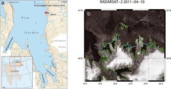
Fig. 1. (a) Map of Rijpfjorden. Star indicates the IMB; circle indicates the weather station. Inset shows the Svalbard archipelago. Black rectangle indicates the region of Rijpfjorden; red rectangle indicates the region of northern Svalbard. (b) RADARSAT image of northern Svalbard on 10 April 2011. Green lines show the coastlines, light blue lines represent level landfast ice edges and white areas are glaciers.

2. Measurements

In winter and spring 2010/11, Rijpfjorden was covered by sea ice from early November 2010 to 11 July 2011. To monitor sea-ice evolution in spring, an ice mass-balance buoy (IMB) was deployed for ∼2.5 months from April toJune 2011. The IMB can autonomously delineate the thermodynamic changes of ice mass balance (Reference Richter-Menge, Perovich, Elder, Claffey, Rigor and OrtmeyerRichter-Menge and others, 2006). It includes three components: a thermistor string, a sonar mast and a surface unit (Fig. 2). The thermistor string is ∼4.5m long with 3 × 1.5 m PVC rods to record vertical temperature profiles (every 0.1 m) in the air, snow, ice and the under-ice water every 4 hours. The sonar mast includes a downward-looking ultrasonic sensor in the air and an upward-looking sonar under the ice to measure distances to the snow surface and to the ice bottom, respectively, every 4 hours. The surface unit includes a barometer for barometric pressure, a temperature sensor for air temperature, a Campbell scientific data logger for data storage and an Iridium transmitter to transfer data via satellite every hour. On 10 April 2011, the IMB was deployed in Rijpfjorden (Fig. 1) at 80.28 N, 22.58 E (∼350m from the shore) when the landfast ice became safe to work on and access was possible (Fig. 1b). When the IMB was retrieved on 26 June 2011, the components of the buoy were still standing upright and frozen solid in the ice.

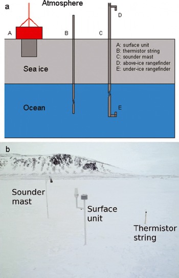
Fig. 2. (a) Schematic of the IMB and (b) photograph of the IMB during deployment in Rijpfjorden in 2011.

Ice cores were collected at the sonar mast site during the IMB deployment and at a location ∼5–10m away from the surface unit when the IMB was retrieved. When deploying the IMB, snow depth, ice thickness and freeboard were measured at the thermistor string and the sonar mast sites. In addition, they were also measured every 5 m along a north-south-oriented 50 m long transect near the IMB site on three occasions: during the IMB deployment on 10 April 2011, during a revisit of the site on 7 May 2011, and while recovering the IMB on 26 June 2011. Snow depth was measured with a metal stake, and ice thickness and freeboard were measured conventionally from drillholes using an ice auger (0.05 m diameter) and a thickness-gauge tape measure (resolution 0.01 m). Table 1 summarizes the measurements performed in Rijpfjorden in the period 10 April–26 June 2011.

Table 1. Overview of measurements in Rijpfjorden between 10 April and 26 June 2011

Ice properties, including temperature, salinity and ice texture, as well as oxygen isotopic composition (δ¹⁸O), were analyzed in the field and in laboratories. Ice temperature was measured in the field immediately after the ice core was collected. Ice texture analysis was performed on thick and thin sections of the cores in a cold laboratory. The remaining cores after the thin and thick section preparation were cut into segments according to stratigraphic units and melted for ice salinity and δ¹⁸O measurement. The ice salinity was determined from the melted samples using a temperature-compensated conductivity meter and UNESCO algorithms (1983). δ¹⁸O was analyzed using a Thermo Fisher Scientific Delta V Advantage mass spectrometer with Gasbench II, and its values are reported in per mil (%) relative to the Vienna Standard Mean Ocean Water (VSMOW) standard.

Meteorological parameters were recorded at an automatic weather station (http://www.unis.no/20_research/2060_online_env_data/weatherstations.htm) located on the shore of Rijpfjorden ∼430 m southeast of the IMB site (Fig. 1a). They include air temperature, wind speed, wind direction, relative humidity, air pressure and photosynthetically active radiation (PAR). The wind sensor at the weather station did not function properly after 18 March 2011. Therefore no wind speed data were recorded for the period of the IMB operation.

3. Results

3.1. Meteorological conditions

Air temperature recorded at the shore-based weather station (at a height of 4.5 m above ground) and the IMB (at a height of 1.0 m) compared well, although the weather-station-derived air temperature was slightly above that measured at the IMB (Fig. 3a). Typically, the air temperature was below 0°C from 10 April to 26 June 2011 in Rijpfjorden. The lowest temperature recorded was below –20°C (IMB: –23°C; weather station: –21 °C) between 10 and 20 April 2011. There were five warm spells between 20 April and 15 May 2011, with temperatures up to +5°C around 25 April. From mid-May the temperature gradually increased from below –10°C, and by the end of May the temperature fluctuated around 0°C. Although there were no wind speed data from 10 April to 26 June 2011, air-pressure data (Fig. 3b) showed low-pressure (before 20 April) and high-pressure (13 May; 10 June) systems passing through in this period. The prevailing winds were northerly (direction 0–30˚; Fig. 3c), from the mouth of the fjord towards its head.

Fig. 3. (a) Air temperature recorded at the weather station on shore and at the IMB site, (b) air pressure and (c) histogram of wind direction in Rijpfjorden between 10 April and 26 June 2011.

3.2. In situ snow depth, ice thickness and freeboard measurements along 5 0 m transect

Snow depth and ice thickness were variable along the 50 m transect, especially in the second half of the transect line and later in the season (Fig. 4). At the first visit on 10 April 2011, the difference between the maximum and minimum ice thickness was 0.12 m. On 7 May 2011, that difference had increased to 0.20 m, and on 26 June 2011 it was as much as 0.37 m, almost 46% of the average ice thickness of 0.81 m. The more variable ice thickness on 26 June 2011 might be related to formation of superimposed ice in June (see Section 4). The spatial variability of snow depth was relatively large on 10 April 2011, with deep snow observed at the starting point and at 40 m distance along the transect. On 7 May 2011, snow surface was relatively homogeneous along the transect. The mean and standard deviation of snow and ice thickness (see Fig. 9 below) are calculated along the 50 m transect on three occasions. Sea ice was thinnest on 10 April 2011, with a mean thickness of 0.68 ± 0.04 m. It became thicker on 7 May 2011, with a mean thickness of 0.78± 0.07 m, and somewhat thicker on 26 June 2011, with a mean thickness of 0.81 ± 0.10 m. In contrast, snow was thickest on 10 April 2011, with a mean thickness of 0.19± 0.07 m. It was thinner in May and June, with mean thicknesses of 0.10 ± 0.04 and 0.09 ± 0.06 m, respectively.

Fig. 4. Variations of snow and ice thickness and freeboard with distance along the 50 m transect on (a) 10 April, (b) 7 May and (c) 26 June 2011. Zero depth on the y-axis represents the water level.

Ice freeboard, the distance between the water level and the ice surface, also varied in space and time (Fig. 4), particularly later in the season. Negative freeboards were measured on all three occasions, with larger negative freeboards on the last two occasions. In particular, large negative freeboards were observed at 40 and 45 m on 7 May 2011 and at 35 m on 26 June 2011, which might be the result of reading errors due to difficulties in determining the snow–ice interface when making in situ measurements (see Section 4).

3.3. IMB-derived snow depth and ice thickness

The downward-looking ultrasonic sensor of the IMB generally worked well, with only a few outliers (Fig. 5). The under-ice sonar worked well until 5 May 2011; between 5 May and 10 June the sonar measured very short distances to the ice base (Fig. 5). Thereafter it again measured similar distances relative to prior to 5 May. When retrieving the IMB on 26 June 2011, all the components of the IMB, including the sonar mast, sat upright and were still frozen solid in the ice. Therefore, it can be rejected that the short distances to the ice base (Fig. 5) resulted from movements of the sonar mast. A possible explanation for the short under-ice distances between 5 May and 10 June is false reflections of the sound wave from ice formation around one of the PVC pipe couplings above the sonar and below the ice. Therefore, the erroneous distances recorded between 5 May and 10 June 2011 are excluded from the analysis and interpretation.

Fig. 5. Measured distances to snow surface and ice bottom by IMB sounders. The recorded erroneous distances (blue crosses) are excluded from the analysis.

Assuming no height change in the snow–ice interface relative to the sonar and the ultrasonic sensor after IMB deployment, we can derive both snow depth and ice thickness from the distances measured by the IMB and the initial in situ snow depth and ice thickness at the IMB site. However, any changes in snow–ice interface after IMB deployment, such as formation of snow ice or superimposed ice, could result in overestimation/underestimation of snow depth/ice thickness. When deploying the IMB (10 April 2011), in situ snow depth and ice thickness were 0.23 and 0.73 m, respectively, at the sonar mast. The initial distances to the snow surface and ice bottom were 1.28 and 4.70 m, respectively.

Figure 6 shows the IMB-derived snow depth and ice thickness. The IMB-derived snow depth was generally <0.25 m before 24 April 2011 and showed little change (Fig. 6). It decreased by ∼0.05 m for a short period around 25 April 2011 as the air temperature increased above 0°C (Fig. 3a). Afterwards, new snow fell and accumulated. The IMB-derived snow depth increased to ∼0.39m by 9 June 2011. After that, snow started to melt when the air temperature fluctuated around 0°C, and melted faster after 10 June 2011 when the air temperature was >0°C. The IMB-derived snow depth was 0.17 m on the day of IMB retrieval. The IMB-derived ice thickness was stable before 5 May 2011, at ∼0.73 m, indicating no ablation or accretion at the ice bottom. Afterwards, the IMB-derived ice thickness started to decrease as the under-ice water became warmer, providing heat to melt the ice base. It decreased to 0.67 m by 11 June 2011. After 11 June, the IMB-derived ice thickness seems to increase, which we explain as sonic echoes from the interface between a freshwater layer under the ice and more saline water above the under-ice sonar (see Section 4).

Fig. 6. IMB-derived snow (grey shading) and ice (white circles) thickness and ice/under-ice water temperature (coloured shading). The zero line is the snow–ice interface (at the start of the deployment and assuming no change in the ice–snow interface). The erroneous ice thickness after 11 June 2011 is highlighted with black crosses.

3.4. Sea-ice texture, salinity and temperature, and oxygen isotopic composition

The retrieved ice cores were 0.73 (10 April) and 0.80m (26 June) long. On 10 April 2011, the top 0.04 m of the ice consisted of granular ice, followed by columnar ice below (Fig. 7a). This is a typical stratigraphy reflecting relatively calm ice growth conditions, as also observed in Kongsfjorden on the western side of Svalbard (Reference Gerland, Winther, Örbek and IvanovGerland and others, 1999) and in Arctic landfast sea ice (Reference Kawamura, Shirasawa and KobinataKawamura and others, 2001). The entire ice core had positive δ¹⁸O values between 0.74% and 2.45%, with the granular layer having the lowest value in the ice (Fig. 7c). This can be related to a sea-water value of 0.1 ±0.1% (n=12) observed in late summer 2010 in the fjord, as the values in the columnar ice correspond well with the expected oxygen isotopic fractionation of ∼2.1‰ during sea-ice formation, as reported by Reference Melling and MooreMelling and Moore (1995). The surface layer of granular ice increased to a thickness of 0.10 m by 26 June 2011 (Fig. 7b). This suggests that a 0.06 m layer of granular ice had formed at the surface from 10 April to 26 June 2011. On 26 June, δ¹⁸O values were in general lower than on 10 April. They ranged from –10.87% to 1.84%, with negative values in the 0.10 m layers at the ice surface and the bottom. The very low negative values at the surface correspond to the granular ice layer. Sea-ice salinity was lower on 26 June than on 10 April (Fig. 7d), the explanation for which is related to melting processes. In particular, the 0.06 m of new granular ice on the surface had the lowest salinity, about 0.4. In addition, the bottom 0.10m also had low salinity, about 0.6. Sea-ice temperature increased from 10 April to 26 June 2011 (Figs 6 and 7e). On 10 April 2011, the ice temperature was below –2°C with a minimum at the ice surface. On 26 June 2011, the in situ ice temperature profile was C-shaped, with the middle part (0.15–0.55m) below 0°C and the bottom parts (0.65–0.75m) equal to 0°C. The IMB-recorded ice temperature on the same day also showed a C-type profile, with all values below 0°C. The discrepancy between the in situ and IMB-recorded ice temperature at the bottom could be related to the ambient conditions for the ice-core measurement, since it was relatively warm (3–5°C).

Fig. 7. (a, b) Photographs of ice-core thin sections with crossed polarizers: (a) on 10 April and (b) sea-ice texture on 26 June. (c) δ¹⁸O, (d) salinity and (e) temperature profiles on 10 April and 26 June 2011. The zero depth refers to the snow–ice interface.

4. Discussion

Large negative freeboards were observed as a part of the direct measurements in drilling holes along the 50 m transect on 7 May and 26 June 2011. In late spring, with increasing solar radiation and air temperatures fluctuating around 0°C, it was difficult to determine the snow-ice interface when making in situ measurements due to deteriorated ice, metamorphosed snow and ice lenses within the snow or at the snow-ice interface.

Based on the ice-core analysis, from April to June 2011 a layer of granular ice of 0.06 m thickness formed at the ice surface. The low salinity and negative δ¹⁸O values at the ice top on 26 June 2011 suggested that the layer at the surface was superimposed ice (e.g. Reference Kawamura, Shirasawa and KobinataKawamura and others, 2001; Reference Granskog, Vihma, Pirazzini and ChengGranskog and others, 2006); further freeboard was generally positive, not supporting snow-ice formation. Therefore, formation of superimposed ice very likely resulted from refreezing of snow meltwater. The IMB-derived snow depth decreased by ∼0.05 m around 25 April 2011 when the air temperature was above 0°C and ∼0.22 m after 9 June 2011 when the air temperature was close to 0°C. Despite the fact that the air temperature was mostly <0°C between 9 and 20 June 2011, the IMB-derived snow depth decreased due to radiative heating within the snow (Reference ColbeckColbeck, 1989). Snow meltwater can percolate down through the snow and accumulate at the ice surface, refreezing to form superimposed ice due to the colder ice below (Reference Granskog, Vihma, Pirazzini and ChengGranskog and others, 2006). Assuming ratios of snow transformed to superimposed ice of about 4 : 1 (in Kongsfjorden; Reference Nicolaus, Haas and BareissNicolaus and others, 2003) and 2 : 1 (in the Baltic Sea; Reference Granskog, Vihma, Pirazzini and ChengGranskog and others, 2006), 0.05 m of snowmelt around 25 April 2011 and 0.22 m snowmelt after 9 June 2011 would form layers of superimposed ice of ∼0.01–0.025 m around 25 April and ∼0.05–0.12 m after 9 June. This may suggest that the superimposed ice of 0.06 m thickness formed mainly after 9 June 2011.

Formation of superimposed ice at the ice surface changed the height of the snow-ice interface. This makes the assumption of no changes in the snow-ice interface in June unreasonable and leads to an overestimation of IMB-derived snow depth, especially after 9 June 2011. The increased spatial variability in the in situ ice thickness and freeboard observed on 26 June 2011 might be attributed to formation of superimposed ice.

In situ measurements suggest that sea ice grew 0.07 m (ice-core analysis) and 0.13 m (average along the 50 m transect) in the period 10 April–26 June 2011. When excluding superimposed ice, the sea-ice thickness was more or less unchanged (grew by 0.01 or 0.06 m) at the ice base. The spatial variability of fast-ice thickness might be a major factor leading to these numbers and differences. Sea-ice thickness derived from IMB sonar data suggested a significant increase in ice thickness after about 11 June 2011. If the reflections of the under-ice sonar come from the ice–water interface, ice thickness would have increased by 0.18m at the bottom alone. However, the air temperature was not sufficient to support thermodynamic ice growth during this time (Fig. 6). If there had been a sudden growth at the ice base, it would also be apparent in the ice cores. However, the ice-core analysis shows only an increase in the thickness of the surface granular ice followed by columnar ice (Fig. 7a and b). Therefore, the IMB-derived ice thickness is not seen as valid after 11 June. In late spring, a layer of fresh water under the ice, possibly originating from melting snow and sea ice or nearby glaciers, has been observed underlying the fast ice in Kongsfjorden, a fjord in western Svalbard. The highly negative δ¹⁸O values and low salinity in the ice on 26 June 2011 (Fig. 7) imply that either the ice has been flushed with surface snow meltwater or it has been infiltrated by fresher waters (likely of snowmelt origin on top of the ice or from nearby runoff from glaciers) from below. Such a scenario was observed on the coast of Ellesmere Island, Arctic Canada, where fast ice grows into a stratified layer of fresh water with low salinity and δ¹⁸O (Reference Jeffries and KrouseJeffries and Krouse, 1988). The interface of the fresh water and the more saline water below could work as a reflector for the sonar signals of the IMB under-ice sonar (see Fig. 8) and thereby lead to the decreased distances from the sonar to the reflector after 11 June 2011. Another possibility for explaining these sonar measurements is double diffusive convection of heat and salt occurring at the interface between the fresh water and the underlying salty water. The heat diffusivity is much greater than the salt, possibly leading to supercooling, freezing and a false bottom (Untersteiner and Badgley, 1958; Reference Martin and KauffmanMartin and Kauffman, 1974; Reference Eicken, Krouse, Kadko and PerovichEicken and others, 2002). False bottoms are the only significant source of ice formation in the Arctic during summer and may play a significant role in the summer heat budget of the ice–ocean system (Reference Notz, McPhee, Worster, Maykut, Schlunzen and EickenNotz and others, 2003).

Fig. 8. Sketch of the interface of fresh water and more saline water (thick white line) acting as a reflector for the sonar signal. Arrows indicate a sound pulse from the under-ice sonar travelling through the sea water, reflecting off the interface of the fresh water and the salty water and returning to the under-ice sonar.

The in situ and IMB-derived snow depth and ice thicknesses from 10 April to 26 June 2011 are summarized in Figure 9. The IMB-derived snow depth was adjusted by assuming that 0.06 m of superimposed ice formed on 9 June (hence the jump in snow thickness on 9 June) and the IMB-derived ice thickness after 11 June was excluded. The mean in situ snow and ice thicknesses are calculated from the measurements at the IMB site. The IMB-derived snow depth and ice thickness are generally in good agreement with the in situ measurements along the 50 m transect and at the IMB site and the ice-core analysis. On 7 May 2011, the IMB-derived snow depth was higher than the mean in situ measurement along the 50 m transect. This was because of the difficulty in determining the snow–ice interface due to ice lenses and slush layers in the snow when conducting the in situ measurements along the 50 m transect, as mentioned above. On the same date, the IMB-derived ice thickness is slightly lower than the mean in situ measurement along the 50m transect. Taking into account the large spatial variability of ice thickness along the 50 m transect, it is still in the range of the standard deviation of the in situ measurements.

Fig. 9. Summary of IMB-derived and in situ snow and ice thicknesses from 10 April to 26 June 2011: IMB (dots), 50 m transect (squares) and standard deviation (error bars) at the IMB site (diamond and hexagram; note the hexagram overlain by the filled square) and ice core (grey columns with grey lines). The IMB-derived snow thickness takes into account the formation of superimposed ice (by adjusting the derived snow thickness by 0.06 m after 9 June, indicated by the black arrow). The erroneous IMB-derived ice thicknesses were excluded.

These findings might help to improve IMB measurements in the future, especially with regard to the under-ice sonar, and may also provide solutions to account for formation of snow ice and superimposed ice, which may become more frequent in thinner and wetter ice regimes. False reflections due to ice formation around the PVC pipe couplings under the ice were reduced in the meantime by using a different type of coupling.

Conclusions

A combination of automated-autonomous and manned in situ measurements of sea ice in Rijpfjorden revealed large temporal and spatial variability of snow and ice thickness. In situ measurements, IMB-derived data and ice-core analysis together provide information about thermodynamic changes in the ice mass balance and indicate possible sources of error in the IMB recordings.

The observations show changes in the snow and at the snow–ice interface during a warm spell and after the onset of melt in spring. Snowmelt occurred around 25 April and after 9 June 2011. Melted snow transformed into a 0.06 m thick layer of superimposed ice at the snow–ice surface, mainly after 9 June 2011. Formation of superimposed ice changed the level of the snow–ice interface relative to the original ice surface and made unreasonable the assumption of no change in the height of the snow–ice interface; consequently, after 9 June 2011, the IMB recordings would overestimate the snow thickness. After subtracting the superimposed ice thickness, the IMB-derived snow depth (0.11 m) is in agreement with the mean of the in situ measurement (0.09 m) along the 50 m transect (Fig. 9) on the day of IMB retrieval (26 June 2011). When the observations started, the main phase of thermodynamic freezing was already completed. The measurements along the 50 m transect showed lateral variability in the fast ice, similar to spatial variability observed on level fast ice in other Svalbard fjords (Reference Gerland and RennerGerland and Renner, 2007; Reference Hendricks, Gerland, Smedsrud, Haas, Pfaffhuber and NilsenHendricks and others, 2011). Under-ice sonar measurements of the IMB at the end of the observation period indicate that possibly a freshwater layer under the ice generates false reflections, which can be misinterpreted as ice growth, or they indicate the existence of false bottoms, which may lead to longer-lasting sea ice in the fjord. It is interesting to apply IMBs in different polar environments, such as sheltered fjord areas, where stratification below the ice from land runoff can occur.