


Introduction
Sea-ice extent and concentration are monitored routinely using passive microwave techniques (e.g. Reference Gloersen and CampbellGloersen and Campbell, 1991; Reference Johannessen, Shalina and MilesJohannessen and others, 1999). Ice thickness, which is the second factor in the total sea-ice volume, and hence the Arctic sea-ice mass-balance estimates, is more complicated to obtain from satellite observations (Reference Sandven and JohannessenSandven and Johannessen, 2006). Fram Strait is by far the most important passage for sea-ice export from the Arctic. Therefore thickness estimates from this area are of special scientific interest.
The common approach to determining sea-ice thickness from satellites is via measurement of the elevation difference between the ice and the water surface (freeboard, h f ), or the snow and the water surface (the sum of freeboard and snow thickness, h s, here called snow freeboard, h sf = h f +h s). the two types of satellite altimeters utilized for freeboard/snow-freeboard detection are radar (Reference Laxon, Peacock and SmithLaxon and others, 2003; Reference Giles, Laxon and WorbyGiles and others, 2008a,Reference Giles, Laxon and Ridoutb) and, more recently, laser-based altimeters (Reference KurtzKurtz and others, 2009; Reference Kwok and RothrockKwok and Rothrock, 2009; Reference Spreen, Kern, Stammer and HansenSpreen and others, 2009). Both give promising spatial and temporal patterns consistent with submarine data, but also present challenges, discussed below.
Radar altimeters detect h f , assuming a snow layer transparent to microwaves. Laser pulses instead reflect from the snow surface, and therefore laser altimeters yield h sf . the conversion to ice thickness, h i (Equation (1) for radar and Equation (2) for laser), is based on the assumption that the freeboard and snow freeboard are determined by the hydrostatic balance:
and
Assumptions about the snow conditions (thickness, h s, and density, ρ s), as well as the sea-ice and sea-water densities (ρ i and ρ w, respectively), are therefore needed.
Due to the labour-intensive nature of data collection and the remote locations of interest, both in situ drilling data and data about snow conditions on sea ice in the High Arctic are sparse. Some earlier published work concentrated on detailed studies of individual ice features (e.g. Reference Melling, Topham and RiedelMelling and others, 1993; Reference Bowen and TophamBowen and Topham, 1996; Reference Timco and BurdenTimco and Burden, 1997) or drillings for calibration/validation of sounding techniques for freeboard or draft (e.g. Reference HaasHaas, 2004; Reference Haas, Goebel, Martin, Pfaffling, vo, Wadhams and AmanatidisHaas and others, 2006). the most extensive dataset on drillings and snow conditions on sea ice resulted from Soviet drifting stations and Sever flights (1928–93) (Reference RomanovRomanov, 1996). Reference WarrenWarren and others (1999) (War99 henceforth) compiled the drift station (1954–91) snow data, while Reference Alexandrov, Sandven and JohannessenAlexandrov and others (2010) reviewed the drill measurement data from the Russian Arctic in the 1980s.
Here we present a new set of in situ sea-ice data from thickness drillings, including density measurements of sea ice and snow. the data were collected on drift ice in Fram Strait and the Barents Sea, and on fast ice along the Svalbard coast in the years 1999–2008. Snow and sea-ice thickness and density distributions are presented.
A freely floating ice floe as a whole is in hydrostatic equilibrium, whereas on a point-to-point basis the equilibrium does not necessarily hold (Reference Doronin and KheisinDoronin and Kheisin, 1977). In drift ice, forces caused by mechanical processes with neighbouring ice floes can cause the ice to be out of hydrostatic equilibrium; the same can happen with landfast ice due to interactions with the shore and bottom. In this study, the deviation from hydrostatic balance is examined using drillings aimed at describing the thickness distribution of a floe. the sensitivity of the h i product with the hydrostatic assumption to the uncertainties of the densities, ρ i, ρ s and ρ w, and the snow thickness, h s, is also presented.
Background
Sea-ice and snow properties are known to vary on the scales of the spatial resolution of altimeter data, which is 2–10 km for the Envisat RA-2 radar (Reference Connor, Laxon, Ridout, Krabill and McAdooConnor and others, 2009), 70 m for the Ice, Cloud and land Elevation Satellite (ICESat) Geoscience Laser Altimeter System (GLAS) (Reference KurtzKurtz and others, 2009) and 250m for the CryoSat-2 Synthetic Aperture Radar Interferometric Radar Altimeter (SIRAL) (http://esamultimedia.esa.int/multimedia/publications/BR199 LR. pdf). Integrations performed over these large footprints require knowledge of the distributions of snow and ice parameters at these scales. Furthermore, estimation of the uncertainty related to the deviations from the assumed snow and ice parameters necessitates knowledge of their variation at larger scales.
For estimating h s on Arctic sea ice, the climatology of War99 is most often used. However, this climatology does not cover Fram Strait, and might not represent recent conditions in the rapidly changing Arctic. the other approaches under development for estimating the snowpack on sea ice are: (1) passive microwave techniques with instruments such as the Advanced Microwave Scanning Radiometer (AMSR-E) on board Earth Observing System (EOS) Aqua (Reference KurtzKurtz and others, 2009), (2) concurrent measurements by laser and radar altimetry and (3) model precipitation analysis. Both (1) and (2) suffer from difficulties in combining measurements with very different spatial resolutions. All three techniques require ground data for validation.
Traditionally, the densities, ρ s, ρ i and ρ w, in the altimetry-based h i calculation are kept constant. Other approaches include the formula by Reference KovacsKovacs (1997) for ρ i dependence on ice thickness, and the ρ s seasonal cycle based on War99 climatology. A constant value for the sea-water density, which exhibits relatively little variation in nature, is generally used (Reference Laxon, Peacock and SmithLaxon and others, 2003; Reference Kwok and CunninghamKwok and Cunningham, 2008; Reference Spreen, Kern, Stammer and HansenSpreen and others, 2009).
Laser altimeters have an order-of-magnitude higher spatial resolution than radar altimeters, but are also more sensitive to uncertainty in the measured freeboard. Radar altimetry is better established as a technique, but large challenges remain, especially in understanding the interference of the radar signal with different surfaces, such as in cases with negative freeboard, snow/ice, superimposed ice and ice layers within the snowpack. Both radar and laser altimetry suffer from uncertainty due to the unknown snow load (Reference GilesGiles and others, 2007) and the challenge of defining the local sea-ice surface. Simulations by Reference Tonboe, Pedersen and HaasTonboe and others (2009) show that variability of the radar penetration and the error caused by preferential sampling of certain ice types are error sources as important for radar altimetry as the uncertainties in the parameters affecting the floe buoyancy. Field data on the distribution and temporal variability of sea-ice density, ice types and the density and depth of snow on the ice are essential for validating and calibrating any satellite-based h i products.
The data from the Fram Strait area are particularly valuable for two reasons. First, the ice conditions result both from ice advection and local processes, and are particularly complex due to the strong southward flow. Second, the ice thickness distribution in Fram Strait is of interest as it is the main passage for meridional ice transport from the Arctic basin.
In Situ Sea-Ice Measurements
The dataset presented here consists of in situ drill-hole measurements of ice, snow and freeboard thicknesses (Table 1). Ice densities from sea-ice cores and snow densities from pit studies are also included. the data were collected during several spring and autumn field campaigns in the years 1999–2008. Landfast sea ice in Spitsbergen fjords, coastal sea ice of Svalbard and drift ice in Fram Strait and the Barents Sea (Fig. 1) are all included.

Fig. 1. (a) the ice stations with thickness drillings providing measurements of ice thickness, snow depth and ice freeboard. (b) the ice stations where, in addition to the thickness drillings, snow density (dots) or ice density (circles) were also measured.
Table 1. Data overview. Number of thickness drillings for sea ice, snow and freeboard (h i, h s, h f ) and column measurements of sea-ice and snow densities (ρ i, ρ s). the number of ice-station sites at which the measurements were conducted is given in parentheses. the sources given in the last column include some of the data and description of the expedition in question. Some of the data have not been published before

Typically at an ice-station site, a snow-pit study is conducted to provide the vertical stratigraphy, temperature and density profiles in the snow on the sea ice. Ice corings for temperature, salinity, chlorophyll content and, often, for density are conducted. Thickness drilling transects including snow depth, sea-ice thickness and freeboard measurements, spanning up to 500m in length, are performed. the typical interval of drillings along a transect is 5–35 m. Each ice station consists of 1–31 (typically 5) measurements of ice and snow thicknesses (Table 1). the location and orientation of the transects are chosen to be the most representative of conditions on the floe. Naturally, the regions of thinnest ice are not investigated since the ice must be thick enough to safely work on. Also, the limited number of drillings might not capture the thickness distribution over the whole floe. For further calculations the data are averaged over an ice floe site, which means averaging over the scales of 10–500m. the actual thickness reading has an uncertainty of 1 cm.
The thickness drillings are conducted using, typically, 5–10 cm diameter drills. For ice density, the core pieces, typically 10 cm long, are weighed and the mean density for the site is calculated as an average weighted by the length of each core piece. Sea-ice density measurements made by weighing the core are often subject to a negative bias due to the loss of some of the brine content and deviation from the ideal form (in this case cylindrical) of the sample (Reference Timco and FrederkingTimco and Frederking, 1996). the uncertainty in the density measurements is ∼15 kgm − 3.
For snow density, a known volume (0.5dm3) of snow is collected using a density probe inserted horizontally into the wall of a snow pit, and then weighed. the measurement is repeated along a vertical profile through the snowpack. A weighted average based on the measurement depths is calculated to obtain the mean density through the snowpack. For snow density measurement, the largest cause of bias is the difficulty in filling the density probe without compressing or losing any snow. the estimated uncertainty for ρ s measurement is ∼50 kgm3.
Results and Discussion
The probability density functions (PDFs) calculated for the mean ice (Fig. 2a–c) and snow thickness (Fig. 2d–f) at the ice stations show the characteristics of the different regions and seasons: landfast ice in Svalbard and drift ice in the Barents Sea (all measurements conducted in spring; Fig. 2a and d), spring data from Fram Strait (Fig. 2b and e) and all autumn data (Fig. 2c and f). the data are divided into (1) Fram Strait and (2) eastern data (Svalbard coast and Barents Sea) because (1) is a region characterized by strong ice advection, whereas in (2) the ice evolution is expected to be less influenced by ice-dynamic processes. Note that the measurements taken in autumn are solely from Fram Strait. A non-parametric kernel smoothing regression is used for the PDF estimates.

Fig. 2. PDFs for sea-ice thickness (a–c) and snow-depth (d–f) data pooled to Barents Sea and landfast ice at Svalbard coast (all data collected in spring; a, d), Fram Strait (only spring data; b, e), autumn data (all data collected in Fram Strait; c, f). Mean, standard deviation (std) and number of ice stations (N) for different pools are indicated. Smoothing window bandwidths of 0.15 m (for ice thickness) and 0.05 m (for snow depth) were applied.
Ice properties
The sea ice in Fram Strait contains ice of various ages transported south from the Arctic basin, as well as some locally formed young ice. Therefore the h i is relatively broadly distributed over the thickness range (Fig. 2b), whereas for the landfast ice around Svalbard and the ice in the Barents Sea (Fig. 2a), the PDF is skewed toward the smallest h i. the average h i for Fram Strait is 2.35m (averaged over both seasons), whereas for Svalbard and the Barents Sea it is 0.63 m. the measurements in Fram Strait can be considered representative as they compare well with the earlier reported thicknesses from Fram Strait (Reference Vinje, Nordlund and KvambekkVinje and others, 1998, table 3).
Despite the small number of data points, the thickness-drilling data from the Barents Sea compare well with the drafts reported by Reference AbrahamsenAbrahamsen and others (2006) from mooring upward-looking sonar measurements in the years 1995–96. In the comparison, one needs to account for the thinnest ice, missing in the in situ data. In 1995, the mean draft was ∼0.5m thicker and in 1996 it was very similar to our measurements in 1999. As pointed out by Reference AbrahamsenAbrahamsen and others (2006), sea-ice conditions in the Barents Sea can experience large interannual variability.
The autumn ice thickness data (Fig. 2c, all collected in Fram Strait) are sparse compared with the spring dataset and are dominated by multi-year ice. No thin first-year ice is present in the autumn data, and therefore the average thickness is >3m. For spring the average h i is <2m.
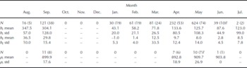
A more detailed view of the seasonal evolution of h i, h f and ρ i, independent of year and region, is presented in Table 2. the thickness maximum due to thermodynamic growth is reached in late spring, which shows up as a sub-maximum of h i in April–May. Similar timing for the h i maximum in Fram Strait is reported by Reference Vinje, Nordlund and KvambekkVinje and others (1998). They observed the ice thickness minimum to occur in September, which in our dataset, on the contrary, is during the season with the greatest thickness.
Table 2. Ice thickness, h i (cm), freeboard, h f (cm) and density, ρ i (kgm − 3). N is the number of measurements (stations) in this study 1999–2008. the measurements are averaged over an ice station before calculating the mean and the standard deviation (std)
Linear robust fits between h f and h i from the thickness drillings (Fig. 3) correspond very well with the work of Reference Ackley, Hibler, Kugzruk, Kovacs and WeeksAckley and others (1976), Reference Vinje and FinnekåsaVinje and Finnekåsa (1986) and Reference Alexandrov, Sandven and JohannessenAlexandrov and others (2010). Figure 3 demonstrates the difference between regions in the Arctic Ocean, as the two datasets collected in the Fram Strait area (Reference Vinje and FinnekåsaVinje and Finnekåsa, 1986, and this study) are more congruent to each other than to Reference Alexandrov, Sandven and JohannessenAlexandrov and others (2010) and Reference Ackley, Hibler, Kugzruk, Kovacs and WeeksAckley and others (1976), whose data are from the Russian Arctic and Beaufort Sea, respectively. the results reported by Reference Vinje and FinnekåsaVinje and Finnekåsa (1986) were obtained from 382 drillings on level ice (not on ridges) during summer months (July–August, 1981–84). Despite the difference in the timing and method, their slope and ours compare well.

Fig. 3. In situ ice thickness as a function of freeboard (dots denote all drillings from this study, circles drillings in Fram Strait), together with linear robust fits (h ifit = 7.37h f + 0.44 (m) and h ifit (FramStrait) = 5.34h f + 1.19 (m)) the black lines are previously published relationships from corresponding in situ data. Many factors, such as the fitting method, the location, timing and method of measurements, differ from those used in this study.
The initial density of the sea ice depends on the conditions whilst freezing. the change in the volume fraction of brine and gases is the mechanism through which ρ i decreases in growing and ageing ice (Reference KovacsKovacs, 1997). This evolution appears only weakly when plotting ρ i against h f (Fig. 4).

Fig. 4. Sea-ice densities as a function of freeboard for 29 cores from Fram Strait, 2005–08. the linear fit (solid line) is strongly influenced by the exceptionally high data point in the lower part of the h f range. Applying a robust linear fit (dashed line) yields a weaker dependence between ice density and freeboard.
The ice density data consist of both first- and multi-year ice in 29 ice cores from Fram Strait, with an average column density of 901.9 kgm − 3, which is lower than the mean of previously reported values (910 kgm − 3; Reference Timco and FrederkingTimco and Frederking, 1996). Fram Strait ice contains some thin newly formed ice, but has a large fraction of multi-year ice. This explains the low densities and perhaps also the relatively high variability (standard deviation between the ice stations 22 kgm − 3). Generally, the variability of ρ i can be expected to be an order of magnitude smaller than that of ρ s.
A comparison of measured and calculated ice thickness (using hydrostatic equilibrium, Equation (1)) is shown in Figure 5. the absolute deviation between the measured and calculated thickness in Fram Strait is, on average, 49 cm (23% of measured h i). In the case of thin first-year ice created by thermodynamic growth without significant dynamic disturbance, the calculated ice thickness mimics the measured one well (Fig. 5a). the deviations between the measured and calculated h i increase slightly toward the thicker part of the thickness range, where the dynamics play a more prominent role. on ridged multi-year ice a larger number of drillings is needed for a representative picture of the thickness distribution. the peaks in Figure 5a indicate the cases where drillings were conducted close to or at a pressure ridge.

Fig. 5. The measured sea-ice thickness (thick curve) and the ice thickness calculated assuming hydrostatic equilibrium (thin curve) for (a) Fram Strait and (b) the Barents Sea and the landfast sea ice at the Svalbard coast. the in situ measured snow and freeboard thicknesses averaged over an ice station (scales of 10–100m) are used for calculation. the sea-water density was set to 1024 kgm − 3 and the snow and sea-ice densities to the averages of the data in this study. the grey area shows the difference between the measured and calculated ice thicknesses. In both graphs the data are sorted by measured ice thickness.
Due to the thinner ice along the Svalbard coast and in the Barents Sea, the deviation from the hydrostatic equilibrium assumption is more critical for their thickness estimate than in the case of the thicker ice in Fram Strait. the measured and calculated ice thicknesses for the Svalbard coast and Barents Sea differ by 36 cm, on average, which is less than three-quarters of the deviation in Fram Strait, but is 48% of measured h i in the area. Purely thermodynamic ice development occurs rarely, but snow-to-ice transformation (Reference Nicolaus, Haas and BareissNicolaus and others, 2003; Reference Gerland, Haas, Nicolaus, Winther and WienckeGerland and others, 2004) complicates the ice evolution and makes the differentiation of snow and ice more convoluted. the landfast ice sites located in protected fjords (Krossfjorden and Kongsfjorden, Svalbard west coast, Fig. 1) are often protected from strong winds and large-scale drift ice motion. Therefore the calculated h i mimics the measured h i better for the Svalbard landfast sites and the Barents Sea than for Fram Strait (Fig. 5). However, a small absolute error is of more importance for thin coastal ice than for thick ice in Fram Strait.
The proximity of the shore and the shallowness of the water bring about particular dynamics affecting the ice freeboard. an example is a situation experienced at Hopen (Fig. 1; Reference Gerland, Renner, Godtliebsen, Divine and LøyningGerland and others, 2008a), where the ice packed toward the shoreline by winds was resting on the bottom. In cases like this (the rightmost values in Fig. 5b), the ice freeboard is not determined by the water buoyancy, so the difference between the measured and calculated ice thicknesses becomes much higher than in cases of pressure ridges (Fig. 5a). This situation is exceptional and occurs only in locations shallower than the draft of the drift ice.
Ratio R
The ratio of mean draft to mean freeboard, R (Reference Wadhams, Tucker, Krabill, Swift, Comiso and DavisWadhams and others, 1992; Wad92 hereafter),
should be related to the densities of sea ice, snow and sea water by
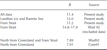
The ratio R is used to describe a certain ice environment, and, furthermore, in the prediction of h i from freeboard. It is not constant, but needs to be tuned for different ice thickness categories; it also varies between seasons and regions (Wad92; Reference Haas, Goebel, Martin, Pfaffling, vo, Wadhams and AmanatidisHaas and others, 2006; Reference Tonboe, Pedersen and HaasTonboe and others, 2009). the ratio calculated for the data from the present study is much higher than R reported earlier for adjacent regions from joint airborne laser and submarine sonar profiles in 1987 by Wad92 and Reference Comiso, Wadhams, Krabill, Swift, Crawford and TuckerComiso and others (1991) (Table 3). In their study, Wad92 excluded data they collected in Fram Strait, stating that the displacement between the draft and freeboard datasets was large. In an area with such heterogeneous ice conditions, the displacement caused their R to deviate significantly from the R in more northern study sections. There is no displacement of the draft and freeboard in our data, but the area-averaging of all the parameters causes R to be large (Table 3), yielding unrealistically high densities (according to Equation (4)) for the floating ice.
Table 3. Ratio R calculated for the thickness data for the whole dataset and the different regions. the data are averaged over the ice stations prior to the calculation (Equation (3)). the literature values from Reference Wadhams, Tucker, Krabill, Swift, Comiso and DavisWadhams and others (1992) (Wad92) and Reference Comiso, Wadhams, Krabill, Swift, Crawford and TuckerComiso and others (1991) (Com91) are added for comparison
Snow conditions
The snow measurements from this study are compared with the climatology of War99 (Table 4). Our study area being south of the region covered by the climatology, differences in climatic conditions between the Soviet NP-stations in War99 and the sites of the present investigation are likely to be significant. Table 4 shows the h s, ρ s and snow water equivalent calculated for different months, independent of year. It is apparent that the data are collected during several field seasons at various locations instead of monitoring the snowpack evolution at one site. Figure 2 shows the PDFs for the observed snow thicknesses. Snow thicknesses in the autumn average 8 cm (Fig. 2f), whereas the spring snow layer on the sea ice is 19 cm thick on average. As Figure 2e shows, the Fram Strait sea-ice h s varies greatly (std dev. 19 cm); this is due to the wind redistribution on an uneven surface. As the sea ice in Fram Strait originates from different regions in the Arctic, the different floes have different weather histories, which is one cause of variability.
Table 4. Snow thickness, h s (cm), density, ρ s (kgm − 3), and water equivalent, SWE (cm), compared with the quadratic fit of the snow climatology by Reference WarrenWarren and others (1999) (War99) for the whole Arctic, 1954–91. N is the number of measurements (stations) of this study, 1999–2008. the h s measurements are averaged over an ice station before calculating the mean and standard deviation (std). For ρ s and SWE, only one measurement per ice station was conducted
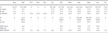
On the landfast sea ice and the Barents Sea the snow cover is notably thinner (h s = 13 cm on average), and varies less than on the Fram Strait ice, most likely due to the even ice surface and shorter accumulation season (Fig. 2d and e). the spring h s in this study are significantly lower than those found by War99 in the central Arctic (Table 4) during 1954–91. the difference is largest for the months with highest h s and less pronounced in the autumn data. Potential explanations for lower h s in our data could be the warmer locations, implying more melting and (together with thinner ice) more snow-to-ice transformation.
The column snow densities average 292.5 kgm − 3 (relative std dev. 0.2), which compares closely to the annual average of 300 kgm − 3 over the Arctic basin reported by War99, increasing from 250 kgm − 3 in September to 320 kgm − 3 in May. Besides this seasonal variation, they reported that ρ s exhibited little geographical variation across the Arctic. the small-scale variation of ρ s, typical for snow parameters due to various depositional (wind and humidity conditions during snowfall) and post-depositional processes (redistribution by snowdrift, snow metamorphosis), is apparent in our data.
Uncertainty of h i estimate
When evaluating sea-ice thickness products from satellite altimetry, it is not sufficient to compare the results solely with submarine or moored ULS measurements. Systematic in situ drilling measurements or measurements by an electromagnetic technique are also needed. Due to the larger fraction of h i under the sea surface than above it, ULS data are less sensitive to, but still subject to, the same errors, caused by snow loading and assumed sea-water and ice densities, as satellite altimetry data.
The equations to calculate the sea-ice thickness product are different for laser and radar altimetry (Equations (1) and (2)), as the laser altimeter beam is assumed to reflect from the snow surface, and the radar waves from the snow and ice interface. Also, the uncertainty in h i and the contributions from the different sources of error differ for radar and laser techniques. Figure 6 shows how uncertainties in the assumptions about snow, ice and sea-water density,

Fig. 6. The sea-ice thickness uncertainty from radar and laser altimetry, as a function of uncertainties in snow and measured freeboard thicknesses ((a) radar, (c) laser) and sea-ice, snow and sea-water densities ((b) radar, (d) laser). As estimates of their natural variability, the solid vertical lines show the standard deviations from the measurements in this study: for snow thickness 0.16 m, for ice density 22 kgm − 3 and for snow density 64 kgm − 3. the dashed vertical lines show variability estimates from the literature, compiled by Reference GilesGiles and others (2007): σh s = 0.11m (Reference WarrenWarren and others, 1999), σh sf = 0.02m (Reference Kwok, Zwally and YiKwok and others, 2004), σh f = 0.03m (Reference Giles and HvidegaardGiles and Hvidegaard, 2006), σρ i = 5 kgm − 3 (Reference Wadhams, Tucker, Krabill, Swift, Comiso and DavisWadhams and others, 1992), σρ s = 3 kgm − 3 (Reference WarrenWarren and others, 1999) and σρ w = 0.5kgm − 3 (Reference Wadhams, Tucker, Krabill, Swift, Comiso and DavisWadhams and others, 1992).
snow thickness and the measured freeboard/snow freeboard propagate to the h i estimate calculated using the hydrostatic law. the total first-order error in the ice thickness (σj being the uncertainty estimate of the jth term) can be calculated using
j = hf , hs, ρi, ρs, ρw for radar,
j = hsf , hs, ρi, ρs, ρw for laser altimetry
We use this equation to look at the contribution of individual error sources to the h i uncertainty.
The bulk of the uncertainty in the h i estimate retrieved from satellite altimetry by both methods is due to the uncertainty in h s fields and the freeboard/snow-freeboard retrieval error (Reference GilesGiles and others, 2007; Reference Kwok and CunninghamKwok and Cunningham, 2008). For radar, the preferential sampling of thinner ice types and the radar penetration variability can cause an error of a similar order of magnitude (Reference Tonboe, Pedersen and HaasTonboe and others, 2009). Relating the observed variability within our dataset and some estimates from other studies (Reference GilesGiles and others, 2007) to the sensitivity calculation for h i, following Equation (5), confirms the importance of the accuracy of the assumed h s in addition to the measured h f or h sf (Fig. 6). the estimate of the total error in h i is ∼20 cm (36 cm) larger for radar (laser) altimetry than that estimated by Reference GilesGiles and others (2007). This is because measured variability in snow load and ice density in this dataset is larger than the literature values they used.
As ice freeboard is smaller than snow freeboard, laser altimetry is more sensitive to measurement errors than radar. the ice thickness dependence on the error of the measured freeboard/snow freeboard for both techniques is significant. In addition to the spatial variability of freeboard in deformed ice, the instrumental inaccuracy and the uncertainty related to the interaction of the altimeter signal with the atmosphere and different types of surfaces contribute to the error. an estimate for snow load uncertainty following Equation (5) brings about an error of 37 cm (radar) and 93 cm (laser), which is much larger than estimated by Reference Alexandrov, Sandven and JohannessenAlexandrov and others (2010), as the data used in their study consist mostly of level ice with thin snow cover.
The h i uncertainties caused by errors in measured freeboard/snow freeboard and estimated snow thickness (Fig. 6a and c) are typically 1–2 orders of magnitude larger than those caused by erroneous assumptions about densities (Fig. 6b and d). the density-related errors are close to identical for radar and laser altimetry. the ice thickness dependence on snow density is low, and therefore the uncertainty is only 9 cm, despite the large variability estimate. the snow-loading uncertainty has a seasonal pattern, peaking at the end of the accumulation season in the spring, and being smallest in the autumn, with least variability in the snow thickness (Table 4). the sea-water density uncertainty is of negligible magnitude (0.5 cm).
The h i uncertainty dependence on ρ i uncertainty is similar to ρ w (Fig. 6), but as the variability is higher, the error grows to 25 cm for both techniques. the earlier studies estimated ρ i variability to be much smaller, based on the estimate of Reference Wadhams, Tucker, Krabill, Swift, Comiso and DavisWadhams and others (1992). Reference Alexandrov, Sandven and JohannessenAlexandrov and others (2010) used the hydrostatic equilibrium to calculate ρ i for Sever drill data and found variability even larger (std dev. of 689 sites 35.7 kgm − 3) than in the present study (std dev. of 22 sites 22.5 kgm − 3). the spatial variability of the sea-ice density needs to be closely studied and considered in the satellite altimeter-based h i.
Averaging over large scales makes the effect of the snow-load and ice density errors less dramatic than for a point estimate. Our data indicate that over the scales of 0.5m to hundreds of metres (the horizontal extent of the drilling transects), the variability of h i, h s, h f and h sf is constant. As the data were collected to give the best possible description of each ice floe at each ice station, the scales of satellite altimeter footprints were not always obtained.
Conclusions
The distributions of the sea-ice thickness and snow depth measured in situ, mostly in Fram Strait, and also the Barents Sea and Svalbard coast, are presented. the measured h i distributions compare well with earlier published work. the h s is significantly lower than the values presented by War99 snow climatology for the Arctic basin.
The in situ drilling data averaged spatially over 10–500m are used to estimate the degree to which the assumption of hydrostatic equilibrium, used in the sea-ice thickness calculation from altimeter data, holds. the hydrostatic equilibrium assumption holds reasonably well for most of the landfast ice, but is less accurate for drift ice. However, for thin ice the relative errors are more prominent than for thick drift ice features in Fram Strait. the deviation between the calculated and measured thickness was on average 49 cm (23% of measured h i) for Fram Strait and 36 cm (48% of measured h i) for the Svalbard coast and Barents Sea.
The measured snow densities compare well with War99 climatology. the sea-ice densities presented large variability and were lower (901.9 kgm − 3 on average) than literature values (Reference Timco and FrederkingTimco and Frederking, 1996; Reference KovacsKovacs, 1997), resulting from the large portion of light multi-year ice included in the present study.
Given the measured spatial variability of the snow and ice parameters, the uncertainty propagating to the calculated sea-ice thickness was estimated. the variability in ice density is found to be larger than previously reported, which brings about an uncertainty of 25 cm in the calculated ice thickness product. Based on our data the error in snow thickness is an even larger source of error (37 cm (radar) and 93 cm (laser altimetry)).
Acknowledgements
We thank everybody who participated in collecting the field data, especially the personnel at the Hopen meteorological station, Sverdrup station in Ny-Ålesund, the crews of S/Y Vagabond, R/V Lance and KV Svalbard. the work was supported by the Norwegian Space Center and European Space Agency through the projects PROgramme de Développement d’EXpériences scientifiques (PRODEX) and CryoSat sea-ice validation and process studies in the European Arctic. the measurements were supported by the following projects funded by the Research Council of Norway: Marine ecosystem consequences of climate induced changes in water masses off West-Spitsbergen (MariClim; project No. 165112/S30), Norwegian–Russian Collaboration on Fast Ice Growth and Decay in Kongsfjorden and Grønfjorden (Svalbard) (NoRu fast ice; project No. 178914); Climate effects of reducing black carbon emissions, Atmosphere–Ice–Ocean interaction studies (AIO; project No. 151447), and iAOOS-Norway: Closing the loop (project No. 176096/S30). EU project DAMOCLES and Center of Ice, Climate and Ecosystems (ICE) at the Norwegian Polar Institute participated in financing the field measurements. We thank A. Nicolaus for structurizing the data and S. Hudson and M. O’Sadnick for useful comments. Reviewers K. Giles, M. Doble, scientific editor N. Hughes, and chief editor M. Granskog are acknowledged for many useful comments that improved the study.


