


1 Introduction
1.1 From quadratic forms to hermitian Morita theory
In the nineteenth century, quadratic forms were the object of many investigations, notably by algebraists such as Gauss, Minkowski, or Kronecker, but were mostly given an arithmetic flavor. The birth of the algebraic theory of quadratic forms over arbitrary fields (of characteristic not $2$
) stems from the seminal 1936 paper of Ernst Witt [Reference Witt27], although a completely unnoticed 1907 paper of Dickson [Reference Dickson7] had actually already made significant advances (see Scharlau’s comment in [Reference Scharlau22]). A key insight of Witt was to shift from the study of individual quadratic forms to the study of the structure they form as a whole. He considers the set
$2$
) stems from the seminal 1936 paper of Ernst Witt [Reference Witt27], although a completely unnoticed 1907 paper of Dickson [Reference Dickson7] had actually already made significant advances (see Scharlau’s comment in [Reference Scharlau22]). A key insight of Witt was to shift from the study of individual quadratic forms to the study of the structure they form as a whole. He considers the set $W(K)$
of isometry classes of quadratic forms over K up to what is now called Witt equivalence, and shows that the direct sum and tensor product of quadratic spaces endow this set with a natural commutative ring structure.
$W(K)$
of isometry classes of quadratic forms over K up to what is now called Witt equivalence, and shows that the direct sum and tensor product of quadratic spaces endow this set with a natural commutative ring structure.
Though quadratic forms over fields were still objects of study, notably through the study of various arithmetic invariants, this algebraic theory of Witt truly started expanding when it was rediscovered in the mid-60s by Pfister (see [Reference Pfister20]), and others such as Arason. It then became abundantly clear that the algebraic structure of the Witt ring was a central element of the theory, and was connected to many subjects of interest, such as Galois cohomology through the Milnor conjecture, or the theory of field orderings, in relation with the much older Artin–Schreier theory. For detailed references on the algebraic theory of quadratic forms, we can cite [Reference Lam16], [Reference Scharlau23], or [Reference Elman, Karpenko and Merkurjev9].
Around the same time, algebraic K-theory was being developed, and the connection with quadratic forms became apparent, as can be seen notably in the foundational work of Bass [Reference Bass and Roy6]. This led to working over general commutative rings, but also to consider not just the Witt ring $W(K)$
, but what we will call the Grothendieck–Witt ring
$W(K)$
, but what we will call the Grothendieck–Witt ring $GW(K)$
(the terminology “Witt–Grothendieck ring” is equally common); one crucial reason Witt introduced the Witt equivalence is that it creates additive inverses in
$GW(K)$
(the terminology “Witt–Grothendieck ring” is equally common); one crucial reason Witt introduced the Witt equivalence is that it creates additive inverses in $W(K)$
, but K-theory taught us that it is very natural to rather add formal inverses. Shortly after that, Bak [Reference Bak, Moss and Thomas4] and Fröhlich and McEvett [Reference Fröhlich and McEvett12] independently started to generalize bilinear forms over commutative rings to
$W(K)$
, but K-theory taught us that it is very natural to rather add formal inverses. Shortly after that, Bak [Reference Bak, Moss and Thomas4] and Fröhlich and McEvett [Reference Fröhlich and McEvett12] independently started to generalize bilinear forms over commutative rings to $\varepsilon $
-hermitian forms over (noncommutative) rings with involution (where
$\varepsilon $
-hermitian forms over (noncommutative) rings with involution (where $\varepsilon $
is a parameter, which is simply equal to
$\varepsilon $
is a parameter, which is simply equal to $\pm 1$
in the classical context of fields with no involution, corresponding to the theory of symmetric and antisymmetric bilinear forms); a more advanced reference is found in [Reference Knus14]. In particular, Fröhlich and McEvett define Witt and Grothendieck–Witt groups
$\pm 1$
in the classical context of fields with no involution, corresponding to the theory of symmetric and antisymmetric bilinear forms); a more advanced reference is found in [Reference Knus14]. In particular, Fröhlich and McEvett define Witt and Grothendieck–Witt groups $W^\varepsilon (A,\sigma )$
and
$W^\varepsilon (A,\sigma )$
and $GW^\varepsilon (A,\sigma )$
; furthermore, they develop an analogue for hermitian modules of the classical Morita theory over rings, which they aptly call hermitian Morita theory. This theory is the central tool used in this article, and we review it in Section 3, although in a different form.
$GW^\varepsilon (A,\sigma )$
; furthermore, they develop an analogue for hermitian modules of the classical Morita theory over rings, which they aptly call hermitian Morita theory. This theory is the central tool used in this article, and we review it in Section 3, although in a different form.
Prominent among rings with involutions are the (finite-dimensional) central simple algebras with involution over fields, which we will thereafter simply call “algebras with involution.” Their study was initiated by Albert in [Reference Albert1] with the context of Riemann surfaces in mind, but found a renewed interest when Weil [Reference Weil26] showed that they can be used to describe the simple algebraic groups over arbitrary fields. A comprehensive treatment of those algebras and their hermitian forms is given in the reference monograph [Reference Knus, Merkurjev, Rost and Tignol15] by Knus et al.
1.2 The idea of the mixed Witt ring
One important caveat in all those generalizations is that when we work over noncommutative rings, we can only speak about (Grothendieck–)Witt groups and not rings. This is simply because there is no tensor product of modules over noncommutative rings. Rather, the tensor product of two A-modules (for example, on the right) is an $(A\otimes A)$
-module. This being said, there is still some compatibility between Witt groups and tensor products: if
$(A\otimes A)$
-module. This being said, there is still some compatibility between Witt groups and tensor products: if $(A,\sigma )$
and
$(A,\sigma )$
and $(B,\tau )$
are algebras with involution over some field with involution
$(B,\tau )$
are algebras with involution over some field with involution $(K,\iota )$
, the tensor product induces maps
$(K,\iota )$
, the tensor product induces maps
 $$ \begin{align*} GW^\varepsilon(A,\sigma)\times GW^{\varepsilon'}(B,\tau)\longrightarrow GW^{\varepsilon\varepsilon'}(A\otimes_K B,\sigma\otimes \tau) \end{align*} $$
(here, $\varepsilon ,\varepsilon '\in K^\times $
are parameters such that
$\varepsilon ,\varepsilon '\in K^\times $
are parameters such that $\varepsilon \iota (\varepsilon )=1$
). This is not surprising if one interprets the Grothendieck–Witt group as the degree
$\varepsilon \iota (\varepsilon )=1$
). This is not surprising if one interprets the Grothendieck–Witt group as the degree $0$
part of hermitian K-theory (see [Reference Bak5] for instance), and it expresses the fact that (Grothendieck–)Witt groups are monoidal functors on some category (which will be made precise).
$0$
part of hermitian K-theory (see [Reference Bak5] for instance), and it expresses the fact that (Grothendieck–)Witt groups are monoidal functors on some category (which will be made precise).
In the special case of algebras with involutions of the first kind (so $\iota =\operatorname {\mathrm {Id}}$
in the notation above), a remarkable phenomenon is that not only do the algebras “have order
$\iota =\operatorname {\mathrm {Id}}$
in the notation above), a remarkable phenomenon is that not only do the algebras “have order $2$
” with respect to Brauer-equivalence, but we have an explicit canonical hermitian Morita equivalence between
$2$
” with respect to Brauer-equivalence, but we have an explicit canonical hermitian Morita equivalence between $(A\otimes _K A,\sigma \otimes \sigma )$
and
$(A\otimes _K A,\sigma \otimes \sigma )$
and $(K,\operatorname {\mathrm {Id}})$
, which means that by general considerations of Morita theory, we get a canonical isomorphism
$(K,\operatorname {\mathrm {Id}})$
, which means that by general considerations of Morita theory, we get a canonical isomorphism
 $$ \begin{align*} GW(A\otimes_K A,\sigma\otimes\sigma) \stackrel{\sim}{\longrightarrow} GW(K). \end{align*} $$
If we combine this with the natural product
 $$ \begin{align*} GW^\varepsilon(A,\sigma)\times GW^\varepsilon(A,\sigma) \to GW(A\otimes_K A,\sigma\otimes \sigma), \end{align*} $$
we get a canonical “mixed” product
 $$ \begin{align*} GW^\varepsilon(A,\sigma)\times GW^\varepsilon(A,\sigma) \to GW(K). \end{align*} $$
In other words, we can define the product of two $\varepsilon $
-hermitian forms, but the result is not a hermitian form, but rather a quadratic form over the base field. It is in that sense that we mean the product is “mixed.” Using the basic fact that
$\varepsilon $
-hermitian forms, but the result is not a hermitian form, but rather a quadratic form over the base field. It is in that sense that we mean the product is “mixed.” Using the basic fact that $GW(K)$
is a ring and
$GW(K)$
is a ring and $GW^\varepsilon (A,\sigma )$
is a
$GW^\varepsilon (A,\sigma )$
is a $GW(K)$
-module, this allows us to construct a
$GW(K)$
-module, this allows us to construct a $\mathbb {Z}/2\mathbb {Z}$
-graded commutative ring
$\mathbb {Z}/2\mathbb {Z}$
-graded commutative ring
 $$ \begin{align*} \widetilde{GW}^\varepsilon(A,\sigma) = GW(K) \oplus GW^\varepsilon(A,\sigma). \end{align*} $$
Actually, it turns out that for functoriality reasons, it is much more convenient to bundle together hermitian and anti-hermitian forms, and rather consider the mixed Grothendieck–Witt ring
 $$ \begin{align*} \widetilde{GW}(A,\sigma) = GW(K) \oplus GW^{-1}(K) \oplus GW^1(A,\sigma) \oplus GW^{-1}(A,\sigma), \end{align*} $$
which is graded over $\Gamma = \mathbb {Z}/2\mathbb {Z}\times \mu _2(K)$
. Of course, the same construction holds for Witt groups, giving the mixed Witt ring
$\Gamma = \mathbb {Z}/2\mathbb {Z}\times \mu _2(K)$
. Of course, the same construction holds for Witt groups, giving the mixed Witt ring
 $$ \begin{align*} \widetilde{W}(A,\sigma) = W(K) \oplus W^1(A,\sigma) \oplus W^{-1}(A,\sigma). \end{align*} $$
A large part of this article is dedicated to showing that these are indeed well-defined commutative rings, and that they are functorial in the sense that any hermitian Morita equivalence between algebras with involution induces a graded ring isomorphism.
It should be mentioned that a very similar construction was made by Lewis in [Reference Lewis18], for the special case where A is a division quaternion algebra, although many key properties, such as associativity and commutativity, are stated without proof. Instead of the involution trace form, Lewis uses the norm form, which is a special feature of quaternion algebras.
We also present a less powerful construction which has the merit of working even for involutions of the second kind: in that case, $(A,\sigma )$
is not its own inverse (up to hermitian Morita equivalence); rather, its inverse is the twisted algebra
$(A,\sigma )$
is not its own inverse (up to hermitian Morita equivalence); rather, its inverse is the twisted algebra $(A^\iota ,\sigma )$
, where the action of K on A is twisted by
$(A^\iota ,\sigma )$
, where the action of K on A is twisted by $\iota $
. Then we can define a
$\iota $
. Then we can define a $\mathbb {Z}$
-graded ring
$\mathbb {Z}$
-graded ring $\widehat {GW}(A,\sigma )$
where the component of degree n is
$\widehat {GW}(A,\sigma )$
where the component of degree n is $GW(A^{\otimes n},\sigma ^{\otimes n})$
if
$GW(A^{\otimes n},\sigma ^{\otimes n})$
if $n\geqslant 0$
and
$n\geqslant 0$
and $GW((A^\iota )^{\otimes (-n)},\sigma ^{\otimes (-n)})$
if
$GW((A^\iota )^{\otimes (-n)},\sigma ^{\otimes (-n)})$
if $n< 0$
; we can “cancel out” the A and
$n< 0$
; we can “cancel out” the A and $A^\iota $
as many times as necessary, so that the product of
$A^\iota $
as many times as necessary, so that the product of $x\in GW(A^{\otimes n},\sigma ^{\otimes n})$
and
$x\in GW(A^{\otimes n},\sigma ^{\otimes n})$
and $y\in GW((A^\iota )^{\otimes m},\sigma ^{\otimes m})$
is in
$y\in GW((A^\iota )^{\otimes m},\sigma ^{\otimes m})$
is in $GW(A^{\otimes n-m},\sigma ^{\otimes n-m})$
if
$GW(A^{\otimes n-m},\sigma ^{\otimes n-m})$
if $n\geqslant m$
, and in
$n\geqslant m$
, and in $GW((A^\iota )^{\otimes m-n},\sigma ^{\otimes m-n})$
otherwise.
$GW((A^\iota )^{\otimes m-n},\sigma ^{\otimes m-n})$
otherwise.
1.3 Content of the article
Our approach in defining and studying our mixed rings is to highlight as much as possible the formal aspects of the construction: it is a consequence of general properties of symmetric monoidal categories, applied to a certain category which encodes hermitian Morita theory. In consequence, the first part is dedicated to general considerations on monoidal categories.
Sections 2.1 and 2.2 are a basic introduction to symmetric monoidal categories, as can be found in any reference on categories, such as the classic [Reference Mac Lane19]. They are here for convenience of readers who are unfamiliar with that theory, as well as to fix some notations.
Section 2.3 contains the technical heart of the article: we explain how a special property of a symmetric monoidal category, which we call strong symmetry (Definition 2.1), allows to coherently choose inverses of objects (Theorem 2.16), and to coherently handle n-torsion of objects (Proposition 2.17). The strong symmetry property was introduced in [Reference Ulbrich24], where it was already used to get a similar result about inverses; our result is basically a reformulation of [Reference Laplaza17, Corollary 4.6 and Proposition 4.7]. This being said, the presentation we give in terms of monoidal functors $\langle \mathbb {Z}\rangle \to \mathbf {C}$
is our own, and we do believe that it sheds an interesting light on those results, by constructing a universal category
$\langle \mathbb {Z}\rangle \to \mathbf {C}$
is our own, and we do believe that it sheds an interesting light on those results, by constructing a universal category $\mathbf {C}^\times $
of inverses in
$\mathbf {C}^\times $
of inverses in $\mathbf {C}$
, and defining the relevant structure as a functor
$\mathbf {C}$
, and defining the relevant structure as a functor $\mathbf {C}\to \mathbf {C}^\times $
which “coherently chooses inverses.” There are many variations in the literature around such “enhanced group structures” on monoidal categories (see [Reference Baez and Lauda3] for more references), and so we give yet another one. On the other hand, Proposition 2.17, which adapts the previous idea to handle n-torsion with monoidal functors
$\mathbf {C}\to \mathbf {C}^\times $
which “coherently chooses inverses.” There are many variations in the literature around such “enhanced group structures” on monoidal categories (see [Reference Baez and Lauda3] for more references), and so we give yet another one. On the other hand, Proposition 2.17, which adapts the previous idea to handle n-torsion with monoidal functors $\langle \mathbb {Z}/n\mathbb {Z}\rangle \to \mathbf {C}$
, is our own, though the basic idea of the proof is very reminiscent of [Reference Joyal and Street13].
$\langle \mathbb {Z}/n\mathbb {Z}\rangle \to \mathbf {C}$
, is our own, though the basic idea of the proof is very reminiscent of [Reference Joyal and Street13].
In Section 2.4, we explain how to construct graded rings (which is our end goal) from monoidal functors. In fact, we explain that an M-graded ring is essentially the same as a lax monoidal functor from the discrete category $\langle M\rangle $
to the category of abelian groups. It is a very simple idea, but we have not found previous uses in the literature. We give slightly refined versions of that statement, which will be adapted to the construction of our mixed rings, in relation with the structures described in the previous section (Corollary 2.20).
$\langle M\rangle $
to the category of abelian groups. It is a very simple idea, but we have not found previous uses in the literature. We give slightly refined versions of that statement, which will be adapted to the construction of our mixed rings, in relation with the structures described in the previous section (Corollary 2.20).
The second part is dedicated to the presentation of our version of hermitian Morita equivalence (in the framework of algebras with involution), which has a strong categorical flavor, so that we can combine it later with the result of the first part.
Section 3.1 exposes the basic theory of hermitian forms over algebras with involution, mostly to fix the terminology and notations. It does not contain anything original beyond some notation, and all the material can be found in [14, Reference Knus, Merkurjev, Rost and Tignol15]. Particular attention should be given to Example 3.5, which presents the canonical Morita equivalence alluded to earlier and which is the basis of our ring construction; it was already introduced in [Reference Fröhlich and McEvett12].
In Section 3.2, we explain how to package hermitian Morita theory in a category $\mathbf {Br}_h(K,\iota )$
. The only thing new is the presentation, as the actual mathematical results can all be found in [Reference Knus14], and actually already in [Reference Fröhlich and McEvett12]. The notion that (classical) Morita theory could be elegantly expressed in a certain
$\mathbf {Br}_h(K,\iota )$
. The only thing new is the presentation, as the actual mathematical results can all be found in [Reference Knus14], and actually already in [Reference Fröhlich and McEvett12]. The notion that (classical) Morita theory could be elegantly expressed in a certain $2$
-category whose morphisms are bimodules is now rather classical in the field of “higher algebra” (see, for instance, [Reference Duskin and Borceux8]) and has been generalized in all sorts of direction (for example, [Reference Vitale25]), but to the best of our knowledge, this is the first time the hermitian version is explicitly written down in practical terms. Note that indeed the natural framework would be to consider a
$2$
-category whose morphisms are bimodules is now rather classical in the field of “higher algebra” (see, for instance, [Reference Duskin and Borceux8]) and has been generalized in all sorts of direction (for example, [Reference Vitale25]), but to the best of our knowledge, this is the first time the hermitian version is explicitly written down in practical terms. Note that indeed the natural framework would be to consider a $2$
-category, where the
$2$
-category, where the $2$
-morphisms are bimodule morphisms, but it is not needed for what follows, so to avoid unnecessary complications, we “truncate” the natural
$2$
-morphisms are bimodule morphisms, but it is not needed for what follows, so to avoid unnecessary complications, we “truncate” the natural $2$
-category to a plain category, at the cost of having morphisms be isometry classes of hermitian bimodules. Since the non-hermitian version is sometimes called the Brauer
$2$
-category to a plain category, at the cost of having morphisms be isometry classes of hermitian bimodules. Since the non-hermitian version is sometimes called the Brauer $2$
-group of a commutative ring, we named this category the hermitian Brauer
$2$
-group of a commutative ring, we named this category the hermitian Brauer $2$
-group.
$2$
-group.
In Section 3.3, we investigate the connection between the usual automorphisms of an algebra with involution and its hermitian Morita self-equivalences. In particular, Proposition 3.9 shows that an algebraic automorphism induces the trivial Morita automorphism if and only if it is inner.
This is used in Section 3.4 to show that $\mathbf {Br}_h(K,\iota )$
is strongly symmetric (Corollary 3.13); the key point is the existence of the ubiquitous Goldman element in a central simple algebra, since it implies that the switching automorphism of
$\mathbf {Br}_h(K,\iota )$
is strongly symmetric (Corollary 3.13); the key point is the existence of the ubiquitous Goldman element in a central simple algebra, since it implies that the switching automorphism of $A\otimes _K A$
is actually inner. This is the crucial result upon which our construction relies, and although ultimately quite simple, it seems to have gone unnoticed until now.
$A\otimes _K A$
is actually inner. This is the crucial result upon which our construction relies, and although ultimately quite simple, it seems to have gone unnoticed until now.
We show in Section 3.5 that for involutions of the first kind, the canonical equivalence defined by the involution trace form does define a coherent $2$
-torsion structure on
$2$
-torsion structure on $\mathbf {Br}_h(K)$
(Theorem 3.14).
$\mathbf {Br}_h(K)$
(Theorem 3.14).
The third part of the article applies the general results of the first part to the category $\mathbf {Br}_h(K,\iota )$
to define our mixed rings.
$\mathbf {Br}_h(K,\iota )$
to define our mixed rings.
Section 4.1 simply defines the underlying (Grothendieck–)Witt groups, and checks that they are functorial with respect to $\mathbf {Br}_h(K,\iota )$
. In order to make them truly functorial as graded objects, a harmless change of labeling is needed (the issue being that anti-hermitian equivalences reverse the signs of hermitian forms instead of preserving them).
$\mathbf {Br}_h(K,\iota )$
. In order to make them truly functorial as graded objects, a harmless change of labeling is needed (the issue being that anti-hermitian equivalences reverse the signs of hermitian forms instead of preserving them).
In Section 4.2, we establish that those functors are actually monoidal, and thus that the whole machinery of Section 2.4 can be used. This leads to the definition of the rings $\widetilde {GW}(A,\sigma )$
and
$\widetilde {GW}(A,\sigma )$
and $\widetilde {W}(A,\sigma )$
(as well as the less interesting
$\widetilde {W}(A,\sigma )$
(as well as the less interesting $\widehat {GW}(A,\sigma )$
and
$\widehat {GW}(A,\sigma )$
and $\widehat {W}(A,\sigma )$
for unitary involutions).
$\widehat {W}(A,\sigma )$
for unitary involutions).
Section 4.3 presents how to handle the (reduced) dimension of hermitian modules, in a way compatible with our graded ring structure.
In order to perform explicit computations in our rings, we describe in Section 4.4 how to multiply diagonal forms; it turns out the result is given by the twisted involution trace forms introduced in [Reference Knus, Merkurjev, Rost and Tignol15, §11] (Proposition 4.9). Whether or not this actually makes the product explicit is a matter of opinion, as those forms are actually quite difficult to compute in practice.
There is at least a case where we can reasonably say that the products are fully computable, namely the case of a quaternion algebra, endowed with its canonical involution. We work this out in Section 4.5 (Proposition 4.12).
Finally, the last Section 4.6, which is the most technical one of the third part, is dedicated to scalar extensions, and especially to establishing a Frobenius reciprocity formula (compare Theorem 4.16 with [Reference Scharlau23, 2.5.6]).
1.4 Perspectives
It should be noted that while in this article we work with algebras over fields, basically everything carries over to Azumaya algebras with involution over general commutative rings. The key ingredient of Corollary 3.13 will still hold in that general context thanks to the existence of the Goldman element. It can even be envisioned to work with Azumaya algebras over schemes, or even locally ringed topos, as studied in [Reference First and Williams11].
In addition to extending the algebras, we could also extend Grothendieck–Witt rings to the whole hermitian K-theory, and actually to simple algebraic K-theory if we forget about the involutions. The fact that such extensions could be easily handled with very little extra legwork is a compelling argument for our general abstract presentation of the mechanisms at play as properties of monoidal categories.
Even considering simply algebras with involutions over fields, we intend to build on the present article in future work to study, among other things: a $\lambda $
-ring structure on
$\lambda $
-ring structure on $\widetilde {GW}(A,\sigma )$
(the existence of which is a strong advantage over
$\widetilde {GW}(A,\sigma )$
(the existence of which is a strong advantage over $\widetilde {W}(A,\sigma )$
); an extension of Artin–Schreier theory for the spectrum of
$\widetilde {W}(A,\sigma )$
); an extension of Artin–Schreier theory for the spectrum of $\widetilde {W}(A,\sigma )$
(related to the work of Astier and Unger in [Reference Astier and Unger2]); and applications of our structure to the construction of cohomological invariants of algebras with involution and algebraic groups.
$\widetilde {W}(A,\sigma )$
(related to the work of Astier and Unger in [Reference Astier and Unger2]); and applications of our structure to the construction of cohomological invariants of algebras with involution and algebraic groups.
1.5 Preliminaries and conventions
We fix a base field K of characteristic not 2, and we identify symmetric bilinear forms and quadratic forms over K, through $b\mapsto q_b$
with
$b\mapsto q_b$
with $q_b(x)=b(x,x)$
. Diagonal quadratic forms are denoted
$q_b(x)=b(x,x)$
. Diagonal quadratic forms are denoted $\langle a_1,\dots ,a_n\rangle $
, with
$\langle a_1,\dots ,a_n\rangle $
, with $a_i\in K^*$
, and
$a_i\in K^*$
, and $\langle \!\langle a_1,\dots ,a_n\rangle \!\rangle $
is the n-fold Pfister form
$\langle \!\langle a_1,\dots ,a_n\rangle \!\rangle $
is the n-fold Pfister form $\langle 1,-a_1\rangle \otimes \cdots \otimes \langle 1,-a_n\rangle $
. We always assume that bilinear forms are nondegenerate.
$\langle 1,-a_1\rangle \otimes \cdots \otimes \langle 1,-a_n\rangle $
. We always assume that bilinear forms are nondegenerate.
All rings are associative and with unit, and ring morphisms preserve the unit. The group of invertible elements of a ring A is denoted $A^\times $
. The opposite ring of A (that is, the ring with the reversed product) is denoted
$A^\times $
. The opposite ring of A (that is, the ring with the reversed product) is denoted $A^{op}$
. Unless otherwise specified, modules are by default modules on the right, and are assumed to be nonzero. Every K-algebra and every module over such an algebra are required to have finite dimension over K. If A and B are K-algebras, a B–A-bimodule is always supposed to be over K, meaning that the right and left actions of K on V coincide. If A is a central simple algebra over K, we write
$A^{op}$
. Unless otherwise specified, modules are by default modules on the right, and are assumed to be nonzero. Every K-algebra and every module over such an algebra are required to have finite dimension over K. If A and B are K-algebras, a B–A-bimodule is always supposed to be over K, meaning that the right and left actions of K on V coincide. If A is a central simple algebra over K, we write $\operatorname {\mathrm {Trd}}_A:A\to K$
for the reduced trace of A.
$\operatorname {\mathrm {Trd}}_A:A\to K$
for the reduced trace of A.
We fix an automorphism $\iota $
of K such that
$\iota $
of K such that $\iota ^2=\operatorname {\mathrm {Id}}$
, and we let
$\iota ^2=\operatorname {\mathrm {Id}}$
, and we let $k=K^\iota $
be the subfield of fixed points. If
$k=K^\iota $
be the subfield of fixed points. If $\iota =\operatorname {\mathrm {Id}}$
, then
$\iota =\operatorname {\mathrm {Id}}$
, then $K=k$
, but if
$K=k$
, but if $\iota \neq \operatorname {\mathrm {Id}}$
, then
$\iota \neq \operatorname {\mathrm {Id}}$
, then $K/k$
is a quadratic extension. Note that we do not include the split case
$K/k$
is a quadratic extension. Note that we do not include the split case $K=k\times k$
, to avoid having to discuss it separately. The reader is encouraged to check that everything would still work in that context.
$K=k\times k$
, to avoid having to discuss it separately. The reader is encouraged to check that everything would still work in that context.
When we say that $(A,\sigma )$
is an algebra with involution over
$(A,\sigma )$
is an algebra with involution over $(K,\iota )$
, we mean that A is a central simple algebra over K, and that
$(K,\iota )$
, we mean that A is a central simple algebra over K, and that $\sigma $
is an involution on A with
$\sigma $
is an involution on A with $\sigma _{|K}=\iota $
, so
$\sigma _{|K}=\iota $
, so $\sigma $
is a k-algebra anti-automorphism of A, with
$\sigma $
is a k-algebra anti-automorphism of A, with $\sigma ^2=\operatorname {\mathrm {Id}}_A$
.
$\sigma ^2=\operatorname {\mathrm {Id}}_A$
.
Recall that the involution $\sigma $
is of the first kind when
$\sigma $
is of the first kind when $\iota = \operatorname {\mathrm {Id}}$
, and is of the second kind (or unitary) otherwise. An involution of the first kind is orthogonal if
$\iota = \operatorname {\mathrm {Id}}$
, and is of the second kind (or unitary) otherwise. An involution of the first kind is orthogonal if $\dim _K(\operatorname {\mathrm {Sym}}(A,\sigma )) = n(n+1)/2$
where n is the degree of A, and it is symplectic if
$\dim _K(\operatorname {\mathrm {Sym}}(A,\sigma )) = n(n+1)/2$
where n is the degree of A, and it is symplectic if $\dim _K(\operatorname {\mathrm {Sym}}(A,\sigma ))=n(n-1)/2$
. In particular,
$\dim _K(\operatorname {\mathrm {Sym}}(A,\sigma ))=n(n-1)/2$
. In particular, $(K,\operatorname {\mathrm {Id}})$
is an algebra with orthogonal involution. A quaternion algebra admits a unique symplectic involution, called its canonical involution.
$(K,\operatorname {\mathrm {Id}})$
is an algebra with orthogonal involution. A quaternion algebra admits a unique symplectic involution, called its canonical involution.
We set $U(K,\iota ) = \{\varepsilon \in K^\times |\varepsilon \iota (\varepsilon )=1\}$
; it is a subgroup of
$U(K,\iota ) = \{\varepsilon \in K^\times |\varepsilon \iota (\varepsilon )=1\}$
; it is a subgroup of $K^\times $
, and when
$K^\times $
, and when $\iota =\operatorname {\mathrm {Id}}$
, it is simply
$\iota =\operatorname {\mathrm {Id}}$
, it is simply $\mu _2(K)$
. If
$\mu _2(K)$
. If $\varepsilon \in U(K,\iota )$
, we define
$\varepsilon \in U(K,\iota )$
, we define $\operatorname {\mathrm {Sym}}^\varepsilon (A,\sigma )$
as the set of
$\operatorname {\mathrm {Sym}}^\varepsilon (A,\sigma )$
as the set of $\varepsilon $
-symmetric elements of A, which satisfy
$\varepsilon $
-symmetric elements of A, which satisfy $\sigma (a)=\varepsilon a$
. We also write
$\sigma (a)=\varepsilon a$
. We also write $\operatorname {\mathrm {Sym}}^\varepsilon (A^\times ,\sigma )$
for the set of invertible
$\operatorname {\mathrm {Sym}}^\varepsilon (A^\times ,\sigma )$
for the set of invertible $\varepsilon $
-symmetric elements.
$\varepsilon $
-symmetric elements.
If $L/K$
is any field extension, and X is an object (algebra, module, involution, hermitian form, etc.) over K, then
$L/K$
is any field extension, and X is an object (algebra, module, involution, hermitian form, etc.) over K, then $X_L$
is the corresponding object over L, obtained by base change.
$X_L$
is the corresponding object over L, obtained by base change.
A semigroup is a set endowed with an associative binary product (so the difference to a monoid is that the semigroup might lack an identity element). The Grothendieck group $G(S)$
of S is the universal solution to the problem of finding a morphism
$G(S)$
of S is the universal solution to the problem of finding a morphism $S\to G$
where G is a group.
$S\to G$
where G is a group.
2 Monoidal categories and graded rings
This section serves both as a quick primer (or reminder) for readers who might be unfamiliar with monoidal categories, and as a presentation of the specific methods used in this article to produce graded rings from those categories. We do assume familiarity with category theory in general. We state most of the general theory without proof, and refer to [Reference Mac Lane19] for more details.
2.1 Monoidal categories
A monoidal category $(\mathbf {C},\otimes ,I)$
(more precisely
$(\mathbf {C},\otimes ,I)$
(more precisely $(\mathbf {C},\otimes ,I,\alpha ,\lambda ,\rho )$
) consists of the data of:
$(\mathbf {C},\otimes ,I,\alpha ,\lambda ,\rho )$
) consists of the data of:
-
• a category C;
-
• a bifunctor $\otimes : \mathbf {C}\times \mathbf {C}\to \mathbf {C}$
(i.e., the expression
$x\otimes y$
is functorial in each variable);
$\otimes : \mathbf {C}\times \mathbf {C}\to \mathbf {C}$
(i.e., the expression
$x\otimes y$
is functorial in each variable); -
• a distinguished unit object
$I\in \mathbf {C}$
; -
• for each triple
$x,y,z\in \mathbf {C}$
, a natural isomorphism
$\alpha _{x,y,z}: x\otimes (y\otimes z) \stackrel {\sim }{\longrightarrow } (x\otimes y)\otimes z$
called associator; -
• for each object
$x\in \mathbf {C}$
, a natural isomorphism
$\lambda _x: I\otimes x\stackrel {\sim }{\longrightarrow } x$
called left unitor; and -
• for each object
$x\in \mathbf {C}$
, a natural isomorphism
$\rho _x: x\otimes I\stackrel {\sim }{\longrightarrow } x$
called right unitor.


The fact that the product is bifunctorial means that for any morphisms $f:x\to y$
and
$f:x\to y$
and $g:x'\to y'$
, we get a well-defined
$g:x'\to y'$
, we get a well-defined $f\otimes g: x\otimes x'\to y\otimes y'$
.
$f\otimes g: x\otimes x'\to y\otimes y'$
.
Those various isomorphisms are required to satisfy certain coherence laws relating one another: the triangle diagram

and the pentagon diagram

The associators and unitors are very much part of the data, although in most natural examples they are the “obvious” isomorphisms, and are rarely actually spelled out in practice. Furthermore, MacLane’s coherence theorem [Reference Mac Lane19, VII.2] guarantees that under the above axioms, there is no ambiguity arising if we omit all parentheses and simplify all products with I, as any two identifications between two different expressions using associators and unitors will actually be equal. Therefore, we will use a more relaxed style of notation, and leave all associators/unitors completely in the background. In particular, we allow ourself to write $x^{\otimes n}$
for any object x and any
$x^{\otimes n}$
for any object x and any $n\in \mathbb {N}$
(with the convention
$n\in \mathbb {N}$
(with the convention $x^{\otimes 0} = I$
). We also often simply say that “
$x^{\otimes 0} = I$
). We also often simply say that “ $\mathbf {C}$
is a monoidal category” when the notations are clear.
$\mathbf {C}$
is a monoidal category” when the notations are clear.
Example 2.1 If R is a commutative ring, then $(R\text {-}\mathbf {Mod},\otimes _R,R)$
and
$(R\text {-}\mathbf {Mod},\otimes _R,R)$
and $(R\text {-}\mathbf {Alg},\otimes _R,R)$
are monoidal categories.
$(R\text {-}\mathbf {Alg},\otimes _R,R)$
are monoidal categories.
Example 2.2 If M is a monoid, then the discrete category $\langle M\rangle $
with M as its underlying set is canonically a monoidal category, the tensor product of objects corresponding to the product in M.
$\langle M\rangle $
with M as its underlying set is canonically a monoidal category, the tensor product of objects corresponding to the product in M.
If $(\mathbf {C},\otimes , I)$
and
$(\mathbf {C},\otimes , I)$
and $(\mathbf {D},\otimes , J)$
are monoidal categories, a (lax) monoidal functor from
$(\mathbf {D},\otimes , J)$
are monoidal categories, a (lax) monoidal functor from $\mathbf {C}$
to
$\mathbf {C}$
to $\mathbf {D}$
consists of the data of:
$\mathbf {D}$
consists of the data of:
-
• a functor
$F: \mathbf {C}\to \mathbf {D}$
; -
• a morphism
$J\to F(I)$
; and -
• for each
$x,y\in \mathbf {C}$
, a morphism
$F(x)\otimes F(y)\to F(x\otimes y)$
.


Those morphisms are once again required to satisfy some coherence laws, which we will not spell out here, in the same spirit as the ones above. When those morphisms are isomorphisms, the monoidal functor is called strong (if they are equalities, it is called strict). Again, the structural morphisms in the definition are often “the obvious ones” and are often left unnamed in practice.
Example 2.3 If $R\to S$
is a commutative ring morphism, then the scalar extension functors
$R\to S$
is a commutative ring morphism, then the scalar extension functors $R\text {-}\mathbf {Mod}\to S\text {-}\mathbf {Mod}$
and
$R\text {-}\mathbf {Mod}\to S\text {-}\mathbf {Mod}$
and $R\text {-}\mathbf {Alg}\to S\text {-}\mathbf {Alg}$
have an obvious strong monoidal structure.
$R\text {-}\mathbf {Alg}\to S\text {-}\mathbf {Alg}$
have an obvious strong monoidal structure.
Example 2.4 Any monoid morphism $M\to N$
induces in an obvious way a strict monoidal functor
$M\to N$
induces in an obvious way a strict monoidal functor $\langle M\rangle \to \langle N\rangle $
.
$\langle M\rangle \to \langle N\rangle $
.
A natural transformation $\varphi : F\to G$
between two monoidal functors
$\varphi : F\to G$
between two monoidal functors $\mathbf {C}\to \mathbf {D}$
is called monoidal if it satisfies the commutative diagrams
$\mathbf {C}\to \mathbf {D}$
is called monoidal if it satisfies the commutative diagrams

and

Note that while being a monoidal category and being a monoidal functor are structures put on top of categories/functors, being a monoidal natural transformation is a property.
Monoidal functors and natural transformations can be composed in the obvious way (the behavior of the structural morphisms in those compositions is straightforward). In particular, we get the expected notions of monoidally isomorphic monoidal functors, and of monoidally equivalent categories (in fact, monoidal categories form a $2$
-category, so all the usual notions can apply without change). The composition of two strong (resp. strict) monoidal functors is again strong (resp. strict).
$2$
-category, so all the usual notions can apply without change). The composition of two strong (resp. strict) monoidal functors is again strong (resp. strict).
Remark 2.5 It is well known (see, for instance, [Reference Etingof, Gelaki, Nikshych and Ostrik10, 1.5.3]) that a strong monoidal functor is a monoidal equivalence if and only if it is an equivalence (in other words, if it has a quasi-inverse, then it also has a monoidal quasi-inverse).
Given two (small) monoidal categories $\mathbf {C}$
and
$\mathbf {C}$
and $\mathbf {D}$
, we define
$\mathbf {D}$
, we define $\operatorname {\mathrm {Hom}}_{\otimes }(\mathbf {C},\mathbf {D})$
(resp.
$\operatorname {\mathrm {Hom}}_{\otimes }(\mathbf {C},\mathbf {D})$
(resp. $\operatorname {\mathrm {LaxHom}}_{\otimes }(\mathbf {C},\mathbf {D})$
) as the category of strong (resp. lax) monoidal functors between the two, with monoidal natural transformations as morphisms. Note that any
$\operatorname {\mathrm {LaxHom}}_{\otimes }(\mathbf {C},\mathbf {D})$
) as the category of strong (resp. lax) monoidal functors between the two, with monoidal natural transformations as morphisms. Note that any $F\in \operatorname {\mathrm {Hom}}_{\otimes }(\mathbf {C},\mathbf {D})$
is canonically isomorphic to some
$F\in \operatorname {\mathrm {Hom}}_{\otimes }(\mathbf {C},\mathbf {D})$
is canonically isomorphic to some $F'$
such that the structural isomorphism
$F'$
such that the structural isomorphism $J\to F'(I)$
is actually the identity, and the structural isomorphisms
$J\to F'(I)$
is actually the identity, and the structural isomorphisms $F'(I)\otimes F'(x)\to F(I\otimes x)\stackrel {\sim }{\rightarrow } F(x)$
and
$F'(I)\otimes F'(x)\to F(I\otimes x)\stackrel {\sim }{\rightarrow } F(x)$
and $F'(x)\otimes F'(I)\to F(x\otimes I)\stackrel {\sim }{\rightarrow } F(x)$
are then identified with the unitors in
$F'(x)\otimes F'(I)\to F(x\otimes I)\stackrel {\sim }{\rightarrow } F(x)$
are then identified with the unitors in $\mathbf {D}$
. Therefore, we will usually implicitly restrict to those functors, which brings no noticeable change to the theory (they form a full subcategory of
$\mathbf {D}$
. Therefore, we will usually implicitly restrict to those functors, which brings no noticeable change to the theory (they form a full subcategory of $\operatorname {\mathrm {Hom}}_{\otimes }(\mathbf {C},\mathbf {D})$
such that the inclusion functor is an equivalence, with a canonical quasi-inverse).
$\operatorname {\mathrm {Hom}}_{\otimes }(\mathbf {C},\mathbf {D})$
such that the inclusion functor is an equivalence, with a canonical quasi-inverse).
Example 2.6 If M and N are monoids, then $\operatorname {\mathrm {Hom}}_{\otimes }(\langle M\rangle ,\langle N\rangle )$
is identified with the set of monoid morphisms
$\operatorname {\mathrm {Hom}}_{\otimes }(\langle M\rangle ,\langle N\rangle )$
is identified with the set of monoid morphisms $M\to N$
.
$M\to N$
.
2.2 Symmetric monoidal categories
If $(\mathbf {C},\otimes ,I)$
is a monoidal category, a symmetric structure on
$(\mathbf {C},\otimes ,I)$
is a monoidal category, a symmetric structure on $\mathbf {C}$
is the data of an isomorphism natural in x and y
$\mathbf {C}$
is the data of an isomorphism natural in x and y
 $$ \begin{align} s_{x,y}: x\otimes y \stackrel{\sim}{\longrightarrow} y\otimes x, \end{align} $$
for all $x,y\in \mathbf {C}$
, which we call the switching morphism (also called “symmetry isomorphism”), satisfying some coherence axioms so that it is compatible with associators and unitors, and very importantly the involution axiom stating that
$x,y\in \mathbf {C}$
, which we call the switching morphism (also called “symmetry isomorphism”), satisfying some coherence axioms so that it is compatible with associators and unitors, and very importantly the involution axiom stating that
 $$ \begin{align} s_{y,x}\circ s_{x,y} = \operatorname{\mathrm{Id}}_{x\otimes y}, \end{align} $$
in other words, the composition
 $$ \begin{align*} x\otimes y\xrightarrow{s_{x,y}} y\otimes x \xrightarrow{s_{y,x}} x\otimes y \end{align*} $$
is the identity of $x\otimes y$
(without this last axiom, the category is only called braided).
$x\otimes y$
(without this last axiom, the category is only called braided).
In a symmetric monoidal category, for any objects $x_1,\dots ,x_n\in \mathbf {C}$
and any permutation
$x_1,\dots ,x_n\in \mathbf {C}$
and any permutation $g\in \mathfrak {S}_n$
, there is a well-defined induced isomorphism
$g\in \mathfrak {S}_n$
, there is a well-defined induced isomorphism
 $$ \begin{align} g_*: x_1\otimes\dots \otimes x_n \stackrel{\sim}{\longrightarrow} x_{g^{-1}(1)}\otimes\dots\otimes x_{g^{-1}(n)}, \end{align} $$
which can be described by applying a switching morphism for each transposition, and in particular there is a canonical group morphism
 $$ \begin{align} \mathfrak{S}_n\to \operatorname{\mathrm{Aut}}_{\mathbf{C}}(x^{\otimes n}) \end{align} $$
for each object $x\in \mathbf {C}$
(in a braided category, we get a morphism from the braid group instead, hence the name).
$x\in \mathbf {C}$
(in a braided category, we get a morphism from the braid group instead, hence the name).
Example 2.7 Categories of modules or algebras are canonically symmetric, the switching morphisms being the obvious ones.
Example 2.8 If M is a monoid, the monoidal category $\langle M\rangle $
has a symmetric structure, necessarily unique, if and only if M is commutative.
$\langle M\rangle $
has a symmetric structure, necessarily unique, if and only if M is commutative.
A monoidal functor F between two symmetric monoidal categories $\mathbf {C}$
and
$\mathbf {C}$
and $\mathbf {D}$
is called symmetric (this time, it is a property and not a structure) if the following diagram commutes for all
$\mathbf {D}$
is called symmetric (this time, it is a property and not a structure) if the following diagram commutes for all $x,y\in \mathbf {C}$
:
$x,y\in \mathbf {C}$
:

Example 2.9 The scalar extension functors on categories of modules or algebras are symmetric monoidal.
A “symmetric monoidal natural transformation” is nothing but a monoidal natural transformation between two symmetric monoidal functors (there is no extra condition involving the symmetric structure). Therefore, we can drop the adjective “symmetric” in that case.
The composition of symmetric monoidal functors is symmetric monoidal (there is again a $2$
-category of symmetric monoidal categories). We adapt the earlier notation, and write
$2$
-category of symmetric monoidal categories). We adapt the earlier notation, and write $\operatorname {\mathrm {Hom}}_{\otimes }^s(\mathbf {C},\mathbf {D})$
(resp.
$\operatorname {\mathrm {Hom}}_{\otimes }^s(\mathbf {C},\mathbf {D})$
(resp. $\operatorname {\mathrm {LaxHom}}_{\otimes }^s(\mathbf {C},\mathbf {D})$
) for the full subcategory of
$\operatorname {\mathrm {LaxHom}}_{\otimes }^s(\mathbf {C},\mathbf {D})$
) for the full subcategory of $\operatorname {\mathrm {Hom}}_{\otimes }(\mathbf {C},\mathbf {D})$
(resp.
$\operatorname {\mathrm {Hom}}_{\otimes }(\mathbf {C},\mathbf {D})$
(resp. $\operatorname {\mathrm {LaxHom}}_{\otimes }(\mathbf {C},\mathbf {D})$
) consisting of the symmetric monoidal functors (provided that
$\operatorname {\mathrm {LaxHom}}_{\otimes }(\mathbf {C},\mathbf {D})$
) consisting of the symmetric monoidal functors (provided that $\mathbf {C}$
and
$\mathbf {C}$
and $\mathbf {D}$
have a symmetric structure, of course).
$\mathbf {D}$
have a symmetric structure, of course).
Remark 2.10 Given a symmetric strong monoidal functor between two symmetric monoidal categories, if it admits a quasi-inverse, then it admits a symmetric monoidal quasi-inverse.
The set of functions from any set X to some monoid M has an obvious pointwise monoid structure, but if X is a monoid itself, then the subset of monoid morphisms is in general not a submonoid, unless M is commutative. Likewise, for any (small) category $\mathbf {C}$
and any (small) monoidal category
$\mathbf {C}$
and any (small) monoidal category $\mathbf {D}$
, the category of functors
$\mathbf {D}$
, the category of functors $\mathrm {Fun}(\mathbf {C},\mathbf {D})$
has a natural “pointwise” monoidal structure, with unit the constant functor to the unit object of
$\mathrm {Fun}(\mathbf {C},\mathbf {D})$
has a natural “pointwise” monoidal structure, with unit the constant functor to the unit object of $\mathbf {D}$
. If
$\mathbf {D}$
. If $\mathbf {C}$
is itself monoidal, then there is a natural forgetful functor
$\mathbf {C}$
is itself monoidal, then there is a natural forgetful functor $\operatorname {\mathrm {Hom}}_{\otimes }(\mathbf {C},\mathbf {D})\to \mathrm {Fun}(\mathbf {C},\mathbf {D})$
, but
$\operatorname {\mathrm {Hom}}_{\otimes }(\mathbf {C},\mathbf {D})\to \mathrm {Fun}(\mathbf {C},\mathbf {D})$
, but $\operatorname {\mathrm {Hom}}_{\otimes }(\mathbf {C},\mathbf {D})$
is not monoidal; however, if
$\operatorname {\mathrm {Hom}}_{\otimes }(\mathbf {C},\mathbf {D})$
is not monoidal; however, if $\mathbf {D}$
is symmetric monoidal, then
$\mathbf {D}$
is symmetric monoidal, then $\operatorname {\mathrm {Hom}}_{\otimes }(\mathbf {C},\mathbf {D})$
becomes a (symmetric) monoidal category,
$\operatorname {\mathrm {Hom}}_{\otimes }(\mathbf {C},\mathbf {D})$
becomes a (symmetric) monoidal category, $\mathrm {Fun}(\mathbf {C},\mathbf {D})$
is naturally symmetric, and
$\mathrm {Fun}(\mathbf {C},\mathbf {D})$
is naturally symmetric, and $\operatorname {\mathrm {Hom}}_{\otimes }(\mathbf {C},\mathbf {D})\to \mathrm {Fun}(\mathbf {C},\mathbf {D})$
is symmetric monoidal. To be precise, given two monoidal functors F and G in
$\operatorname {\mathrm {Hom}}_{\otimes }(\mathbf {C},\mathbf {D})\to \mathrm {Fun}(\mathbf {C},\mathbf {D})$
is symmetric monoidal. To be precise, given two monoidal functors F and G in $\operatorname {\mathrm {Hom}}_{\otimes }(\mathbf {C},\mathbf {D})$
, the functor
$\operatorname {\mathrm {Hom}}_{\otimes }(\mathbf {C},\mathbf {D})$
, the functor $F\otimes G: x\mapsto F(x)\otimes G(x)$
is always well defined in
$F\otimes G: x\mapsto F(x)\otimes G(x)$
is always well defined in $\mathrm {Fun}(\mathbf {C},\mathbf {D})$
(and this does not use that F and G are monoidal), but when
$\mathrm {Fun}(\mathbf {C},\mathbf {D})$
(and this does not use that F and G are monoidal), but when $\mathbf {D}$
is symmetric, we give it a monoidal structure by
$\mathbf {D}$
is symmetric, we give it a monoidal structure by
 $$ \begin{align*} (F(x)\otimes G(x))\otimes (F(y)\otimes G(y)) &\stackrel{\sim}{\longrightarrow} (F(x)\otimes F(y))\otimes (G(x)\otimes G(y))\\ &\qquad \to F(x\otimes y)\otimes G(x\otimes y), \end{align*} $$
where we use the symmetric structure in the first arrow. Therefore, we may speak about the monoidal functor $F\otimes G\in \operatorname {\mathrm {Hom}}_{\otimes }(\mathbf {C},\mathbf {D})$
. Note that
$F\otimes G\in \operatorname {\mathrm {Hom}}_{\otimes }(\mathbf {C},\mathbf {D})$
. Note that $\operatorname {\mathrm {Hom}}_{\otimes }^s(\mathbf {C},\mathbf {D})$
is also then a (symmetric) monoidal subcategory of
$\operatorname {\mathrm {Hom}}_{\otimes }^s(\mathbf {C},\mathbf {D})$
is also then a (symmetric) monoidal subcategory of $\operatorname {\mathrm {Hom}}_{\otimes }(\mathbf {C},\mathbf {D})$
.
$\operatorname {\mathrm {Hom}}_{\otimes }(\mathbf {C},\mathbf {D})$
.
2.3 Strong symmetry, inverses and torsion
For any monoid M, the set of monoid morphisms $N\to M$
has a special interpretation when
$N\to M$
has a special interpretation when $N=\mathbb {N}$
,
$N=\mathbb {N}$
, $\mathbb {Z}$
or
$\mathbb {Z}$
or $\mathbb {Z}/n\mathbb {Z}$
: it gives, respectively, M, the set
$\mathbb {Z}/n\mathbb {Z}$
: it gives, respectively, M, the set $M^\times $
of invertible elements, and the set
$M^\times $
of invertible elements, and the set $M[n]\subset M^\times $
of invertible elements of order dividing n. When M is commutative, those identifications are compatible with the natural monoid structure on the set of morphisms
$M[n]\subset M^\times $
of invertible elements of order dividing n. When M is commutative, those identifications are compatible with the natural monoid structure on the set of morphisms $N\to M$
.
$N\to M$
.
We extend those considerations to monoidal categories; an additional layer of difficulty comes from the fact that one may consider either monoidal or symmetric monoidal functors.
Proposition 2.11 Let $(\mathbf {C},\otimes ,I)$
be a monoidal category. Then the canonical functor
$(\mathbf {C},\otimes ,I)$
be a monoidal category. Then the canonical functor $\operatorname {\mathrm {Hom}}_{\otimes }(\langle \mathbb {N}\rangle , \mathbf {C})\to \mathbf {C}$
defined by
$\operatorname {\mathrm {Hom}}_{\otimes }(\langle \mathbb {N}\rangle , \mathbf {C})\to \mathbf {C}$
defined by $F\mapsto F(1)$
is an equivalence of categories. A quasi-inverse is given by sending
$F\mapsto F(1)$
is an equivalence of categories. A quasi-inverse is given by sending $x\in \mathbf {C}$
to the obvious monoidal functor
$x\in \mathbf {C}$
to the obvious monoidal functor $\Phi _x:\langle \mathbb {N}\rangle \to \mathbf {C}$
such that
$\Phi _x:\langle \mathbb {N}\rangle \to \mathbf {C}$
such that $\Phi _x(n)=x^{\otimes n}$
.
$\Phi _x(n)=x^{\otimes n}$
.
Furthermore, when $\mathbf {C}$
is symmetric, this becomes a symmetric monoidal equivalence if
$\mathbf {C}$
is symmetric, this becomes a symmetric monoidal equivalence if $\operatorname {\mathrm {Hom}}_{\otimes }(\langle \mathbb {N}\rangle , \mathbf {C})$
is endowed with its natural symmetric monoidal structure.
$\operatorname {\mathrm {Hom}}_{\otimes }(\langle \mathbb {N}\rangle , \mathbf {C})$
is endowed with its natural symmetric monoidal structure.
Proof The only thing to check for the equivalence is that if $F: \langle \mathbb {N}\rangle \to \mathbf {C}$
is a strong monoidal functor, then
$F: \langle \mathbb {N}\rangle \to \mathbf {C}$
is a strong monoidal functor, then $\Phi _{F(1)}$
is monoidally isomorphic to F, which is immediate from the axioms of monoidal functors.
$\Phi _{F(1)}$
is monoidally isomorphic to F, which is immediate from the axioms of monoidal functors.
The fact that this equivalence is symmetric monoidal when $\mathbf {C}$
is symmetric is clear given the definition of the symmetric monoidal structure on
$\mathbf {C}$
is symmetric is clear given the definition of the symmetric monoidal structure on $\operatorname {\mathrm {Hom}}_{\otimes }(\langle \mathbb {N}\rangle , \mathbf {C})\to \mathbf {C}$
.▪
$\operatorname {\mathrm {Hom}}_{\otimes }(\langle \mathbb {N}\rangle , \mathbf {C})\to \mathbf {C}$
.▪
2.3.1 Strong symmetry
If $\mathbf {C}$
is symmetric and we want to characterize similarly
$\mathbf {C}$
is symmetric and we want to characterize similarly $\operatorname {\mathrm {Hom}}_{\otimes }^s(\langle \mathbb {N}\rangle , \mathbf {C})$
, we need a definition.
$\operatorname {\mathrm {Hom}}_{\otimes }^s(\langle \mathbb {N}\rangle , \mathbf {C})$
, we need a definition.
Definition 2.1 Let $(\mathbf {C},\otimes ,I)$
be a symmetric monoidal category. An object
$(\mathbf {C},\otimes ,I)$
be a symmetric monoidal category. An object $x\in \mathbf {C}$
is called strongly symmetric if the switching map
$x\in \mathbf {C}$
is called strongly symmetric if the switching map $s_{x,x}$
is the identity of
$s_{x,x}$
is the identity of $x\otimes x$
.
$x\otimes x$
.
We write $\mathbf {C}^{ss}$
for the full subcategory of
$\mathbf {C}^{ss}$
for the full subcategory of $\mathbf {C}$
consisting of the strongly symmetric elements; we say that
$\mathbf {C}$
consisting of the strongly symmetric elements; we say that $\mathbf {C}$
is strongly symmetric if
$\mathbf {C}$
is strongly symmetric if $\mathbf {C}^{ss}=\mathbf {C}$
.
$\mathbf {C}^{ss}=\mathbf {C}$
.
The definition is equivalent to requiring that the canonical group morphism $\mathfrak {S}_n\to \operatorname {\mathrm {Aut}}_{\mathbf {C}}(x^{\otimes n})$
is trivial for
$\mathfrak {S}_n\to \operatorname {\mathrm {Aut}}_{\mathbf {C}}(x^{\otimes n})$
is trivial for $n=2$
(and thus for all n).
$n=2$
(and thus for all n).
Example 2.12 If M is a commutative monoid, then $\langle M\rangle $
is strongly symmetric.
$\langle M\rangle $
is strongly symmetric.
Lemma 2.13 Let $(\mathbf {C},\otimes ,I)$
be a symmetric monoidal category. If
$(\mathbf {C},\otimes ,I)$
be a symmetric monoidal category. If $x\in \mathbf {C}$
is isomorphic to a strongly symmetric element, it is strongly symmetric.
$x\in \mathbf {C}$
is isomorphic to a strongly symmetric element, it is strongly symmetric.
Proof Let $f: x\stackrel {\sim }{\longrightarrow } y$
with y strongly symmetric. Since the switching morphism is natural in each variable, the following diagram commutes:
$f: x\stackrel {\sim }{\longrightarrow } y$
with y strongly symmetric. Since the switching morphism is natural in each variable, the following diagram commutes:

Since $s_{y,y}$
is the identity, so is
$s_{y,y}$
is the identity, so is $s_{x,x}$
.▪
$s_{x,x}$
.▪
Lemma 2.14 Let M be a commutative monoid, and $\mathbf {C}$
a symmetric monoidal category. If
$\mathbf {C}$
a symmetric monoidal category. If $F\in \operatorname {\mathrm {Hom}}_{\otimes }^s(\langle M\rangle , \mathbf {C})$
, then for any
$F\in \operatorname {\mathrm {Hom}}_{\otimes }^s(\langle M\rangle , \mathbf {C})$
, then for any $x\in M$
, the object
$x\in M$
, the object $F(x)\in \mathbf {C}$
is strongly symmetric.
$F(x)\in \mathbf {C}$
is strongly symmetric.
Proof Since F is symmetric, we get the commutative diagram (2.5) (with $y=x$
). The vertical arrows are equal isomorphisms because F is strongly symmetric, and the bottom horizontal arrow is the identity because x is strongly symmetric; therefore, the top horizontal arrow is also the identity, which exactly means that
$y=x$
). The vertical arrows are equal isomorphisms because F is strongly symmetric, and the bottom horizontal arrow is the identity because x is strongly symmetric; therefore, the top horizontal arrow is also the identity, which exactly means that $F(x)$
is strongly symmetric.▪
$F(x)$
is strongly symmetric.▪
When $M=\mathbb {N}$
, there is a form of converse.
$M=\mathbb {N}$
, there is a form of converse.
Proposition 2.15 Under the equivalence $\operatorname {\mathrm {Hom}}_{\otimes }(\langle \mathbb {N}\rangle , \mathbf {C})\simeq \mathbf {C}$
, the essential image of the subcategory
$\operatorname {\mathrm {Hom}}_{\otimes }(\langle \mathbb {N}\rangle , \mathbf {C})\simeq \mathbf {C}$
, the essential image of the subcategory $\operatorname {\mathrm {Hom}}_{\otimes }^s(\langle \mathbb {N}\rangle , \mathbf {C})$
is exactly
$\operatorname {\mathrm {Hom}}_{\otimes }^s(\langle \mathbb {N}\rangle , \mathbf {C})$
is exactly $\mathbf {C}^{ss}$
.
$\mathbf {C}^{ss}$
.
Proof If $x\in \mathbf {C}^{ss}$
, then the canonical
$x\in \mathbf {C}^{ss}$
, then the canonical $\Phi _x: n\mapsto x^{\otimes n}$
is clearly symmetric, so x is in the essential image. Conversely, if x is in the essential image, it is isomorphic to some
$\Phi _x: n\mapsto x^{\otimes n}$
is clearly symmetric, so x is in the essential image. Conversely, if x is in the essential image, it is isomorphic to some $F(1)$
, which is strongly symmetric by Lemma 2.14, so x is strongly symmetric by Lemma 2.13.▪
$F(1)$
, which is strongly symmetric by Lemma 2.14, so x is strongly symmetric by Lemma 2.13.▪
In particular, we see that $\mathbf {C}^{ss}$
is a monoidal subcategory of
$\mathbf {C}^{ss}$
is a monoidal subcategory of $\mathbf {C}$
(which can be shown directly).
$\mathbf {C}$
(which can be shown directly).
2.3.2 Inverses
Definition 2.2 Let $\mathbf {C}$
be a monoidal category. We define its category of inverses
$\mathbf {C}$
be a monoidal category. We define its category of inverses $\mathbf {C}^\times $
as
$\mathbf {C}^\times $
as $\operatorname {\mathrm {Hom}}_{\otimes }(\langle \mathbb {Z}\rangle , \mathbf {C})$
. If
$\operatorname {\mathrm {Hom}}_{\otimes }(\langle \mathbb {Z}\rangle , \mathbf {C})$
. If $\mathbf {C}$
is symmetric, its category of symmetric inverses
$\mathbf {C}$
is symmetric, its category of symmetric inverses $\mathbf {C}^{\times ,s}$
is
$\mathbf {C}^{\times ,s}$
is $\operatorname {\mathrm {Hom}}_{\otimes }^s(\langle \mathbb {Z}\rangle , \mathbf {C})$
.
$\operatorname {\mathrm {Hom}}_{\otimes }^s(\langle \mathbb {Z}\rangle , \mathbf {C})$
.
There is an obvious functor $\mathbf {C}^\times \to \mathbf {C}$
sending F to
$\mathbf {C}^\times \to \mathbf {C}$
sending F to $F(1)$
. Clearly, if
$F(1)$
. Clearly, if $F\in \mathbf {C}^\times $
,
$F\in \mathbf {C}^\times $
, $x=F(1)$
and
$x=F(1)$
and $\overline {x}=F(-1)$
must be “weak inverses,” in the sense that
$\overline {x}=F(-1)$
must be “weak inverses,” in the sense that $x\otimes \overline {x}\simeq \overline {x}\otimes x\simeq I$
. If one unfolds the definition of F, one realizes it is exactly the data of an “adjoint equivalence”
$x\otimes \overline {x}\simeq \overline {x}\otimes x\simeq I$
. If one unfolds the definition of F, one realizes it is exactly the data of an “adjoint equivalence” $(x,\overline {x},\varphi ,\psi )$
where
$(x,\overline {x},\varphi ,\psi )$
where $\varphi : x\otimes \overline {x}\stackrel {\sim }{\rightarrow } I$
and
$\varphi : x\otimes \overline {x}\stackrel {\sim }{\rightarrow } I$
and $\psi : \overline {x}\otimes x\stackrel {\sim }{\rightarrow } I$
fit into some commutative diagrams:
$\psi : \overline {x}\otimes x\stackrel {\sim }{\rightarrow } I$
fit into some commutative diagrams:

It turns out that it is enough to satisfy one of them [Reference Baez and Lauda3]. These kinds of data are well known in the literature, and can be considered as a sort of “coherent inverse” of x. In particular, it follows immediately that the choice of a functor $\mathbf {C}\to \mathbf {C}^\times $
such that the composition
$\mathbf {C}\to \mathbf {C}^\times $
such that the composition $\mathbf {C}\to \mathbf {C}^\times \to \mathbf {C}$
is isomorphic to the identity (which of course can only exist if all objects in
$\mathbf {C}\to \mathbf {C}^\times \to \mathbf {C}$
is isomorphic to the identity (which of course can only exist if all objects in $\mathbf {C}$
are weakly invertible) is equivalent to the choice of a “group structure” (or “gs-category” structure) on
$\mathbf {C}$
are weakly invertible) is equivalent to the choice of a “group structure” (or “gs-category” structure) on $\mathbf {C}$
in the sense of [Reference Laplaza17] (see also [Reference Ulbrich24]). It corresponds to a coherent (functorial) choice of inverses for all objects. In that spirit,
$\mathbf {C}$
in the sense of [Reference Laplaza17] (see also [Reference Ulbrich24]). It corresponds to a coherent (functorial) choice of inverses for all objects. In that spirit, $\mathbf {C}^\times $
is a category which embodies all possible such choices, in a canonical way.
$\mathbf {C}^\times $
is a category which embodies all possible such choices, in a canonical way.
Similarly, if $\mathbf {C}$
is symmetric, a symmetric strong monoidal functor
$\mathbf {C}$
is symmetric, a symmetric strong monoidal functor $\mathbf {C}\to \mathbf {C}^{\times ,s}$
such that the composition
$\mathbf {C}\to \mathbf {C}^{\times ,s}$
such that the composition $\mathbf {C}\to \mathbf {C}^{\times ,s}\to \mathbf {C}$
is monoidally isomorphic to the identity is the same as an “abelian gs-category” structure in the sense of [Reference Laplaza17]. Laplaza shows the following in [Reference Laplaza17, Corollary 4.6 and Proposition 4.7].
$\mathbf {C}\to \mathbf {C}^{\times ,s}\to \mathbf {C}$
is monoidally isomorphic to the identity is the same as an “abelian gs-category” structure in the sense of [Reference Laplaza17]. Laplaza shows the following in [Reference Laplaza17, Corollary 4.6 and Proposition 4.7].
Theorem 2.16 (Laplaza)
Let $\mathbf {C}$
be a monoidal category with every object weakly invertible. Then if we choose for each
$\mathbf {C}$
be a monoidal category with every object weakly invertible. Then if we choose for each $x\in \mathbf {C}$
a weak inverse
$x\in \mathbf {C}$
a weak inverse $\overline {x}$
and an isomorphism
$\overline {x}$
and an isomorphism $x\otimes \overline {x}\stackrel {\sim }{\rightarrow } I$
, there is a unique way to extend that to a gs-category structure
$x\otimes \overline {x}\stackrel {\sim }{\rightarrow } I$
, there is a unique way to extend that to a gs-category structure $\mathbf {C}\to \mathbf {C}^\times $
.
$\mathbf {C}\to \mathbf {C}^\times $
.
Furthermore, it defines an abelian gs-structure $\mathbf {C}\to \mathbf {C}^{\times ,s}$
if and only if
$\mathbf {C}\to \mathbf {C}^{\times ,s}$
if and only if $\mathbf {C}$
is strongly symmetric.
$\mathbf {C}$
is strongly symmetric.
2.3.3 Torsion
Definition 2.3 Let $\mathbf {C}$
be a symmetric monoidal category. Then, for any
$\mathbf {C}$
be a symmetric monoidal category. Then, for any $n\geqslant 2$
, we define the symmetric monoidal category
$n\geqslant 2$
, we define the symmetric monoidal category $\mathbf {C}[n]$
as
$\mathbf {C}[n]$
as $\operatorname {\mathrm {Hom}}_{\otimes }^s(\langle \mathbb {Z}/n\mathbb {Z}\rangle , \mathbf {C})$
. We call it the n-torsion category of
$\operatorname {\mathrm {Hom}}_{\otimes }^s(\langle \mathbb {Z}/n\mathbb {Z}\rangle , \mathbf {C})$
. We call it the n-torsion category of $\mathbf {C}$
.
$\mathbf {C}$
.
Of course, we could have looked at the intermediary step where we only consider $\operatorname {\mathrm {Hom}}_{\otimes }(\langle \mathbb {Z}/n\mathbb {Z}\rangle , \mathbf {C})$
for any monoidal
$\operatorname {\mathrm {Hom}}_{\otimes }(\langle \mathbb {Z}/n\mathbb {Z}\rangle , \mathbf {C})$
for any monoidal $\mathbf {C}$
, but we will not need it, and already in the case of ordinary groups, the notion of n-torsion is much better behaved in a commutative context.
$\mathbf {C}$
, but we will not need it, and already in the case of ordinary groups, the notion of n-torsion is much better behaved in a commutative context.
To any $F\in \mathbf {C}[n]$
is associated a choice of isomorphism
$F\in \mathbf {C}[n]$
is associated a choice of isomorphism $\varphi _x: x^{\otimes n}\stackrel {\sim }{\rightarrow } I$
satisfying some coherence conditions, where
$\varphi _x: x^{\otimes n}\stackrel {\sim }{\rightarrow } I$
satisfying some coherence conditions, where $x=F(1)$
. In particular, x must have weak n-torsion, meaning that
$x=F(1)$
. In particular, x must have weak n-torsion, meaning that $x^{\otimes n}\simeq I$
.
$x^{\otimes n}\simeq I$
.
As before, there is a natural symmetric strong monoidal functor $\mathbf {C}[n]\to \mathbf {C}$
, and we are interested in the choice of a symmetric strong monoidal functor
$\mathbf {C}[n]\to \mathbf {C}$
, and we are interested in the choice of a symmetric strong monoidal functor $\mathbf {C}\to \mathbf {C}[n]$
such that
$\mathbf {C}\to \mathbf {C}[n]$
such that $\mathbf {C}\to \mathbf {C}[n]\to \mathbf {C}$
is monoidally isomorphic to the identity. We call such a choice a “coherent n-torsion” structure on
$\mathbf {C}\to \mathbf {C}[n]\to \mathbf {C}$
is monoidally isomorphic to the identity. We call such a choice a “coherent n-torsion” structure on $\mathbf {C}$
. Clearly, it can only exist if
$\mathbf {C}$
. Clearly, it can only exist if $\mathbf {C}$
is strongly symmetric and all elements have weak n-torsion. Unfortunately, this is no longer sufficient, but we do have the following proposition.
$\mathbf {C}$
is strongly symmetric and all elements have weak n-torsion. Unfortunately, this is no longer sufficient, but we do have the following proposition.
Proposition 2.17 Let $\mathbf {C}$
be a symmetric monoidal category. If
$\mathbf {C}$
be a symmetric monoidal category. If $x\in \mathbf {C}$
is strongly symmetric, any choice of isomorphism
$x\in \mathbf {C}$
is strongly symmetric, any choice of isomorphism $\varphi _x: x^{\otimes n}\stackrel {\sim }{\rightarrow } I$
extends to a unique
$\varphi _x: x^{\otimes n}\stackrel {\sim }{\rightarrow } I$
extends to a unique $F\in \mathbf {C}[n]$
.
$F\in \mathbf {C}[n]$
.
Furthermore, if $\mathbf {C}$
is strongly symmetric, a coherent n-torsion structure is equivalent to the choice of such a
$\mathbf {C}$
is strongly symmetric, a coherent n-torsion structure is equivalent to the choice of such a $\varphi _x$
for all
$\varphi _x$
for all $x\in \mathbf {C}$
, such that for all
$x\in \mathbf {C}$
, such that for all $x,y\in \mathbf {C}$
, we have a commutative diagram
$x,y\in \mathbf {C}$
, we have a commutative diagram

and for each morphism $f:x\to y$
in
$f:x\to y$
in $\mathbf {C}$
:
$\mathbf {C}$
:

Proof It is easy to see that the extension of $\varphi _x$
to F is necessarily unique (up to isomorphism of course), and that it exists exactly when we have the commutative diagram
$\varphi _x$
to F is necessarily unique (up to isomorphism of course), and that it exists exactly when we have the commutative diagram

where the morphism in the top row is given by the identification of $x^{\otimes n}\otimes x$
and
$x^{\otimes n}\otimes x$
and $x\otimes x^{\otimes n}$
with
$x\otimes x^{\otimes n}$
with $x^{\otimes n+1}$
. However, up to the action of the permutation group
$x^{\otimes n+1}$
. However, up to the action of the permutation group $\mathfrak {S}_{n+1}$
on the top row, that diagram always commutes, and since x is strongly symmetric, that action is trivial.
$\mathfrak {S}_{n+1}$
on the top row, that diagram always commutes, and since x is strongly symmetric, that action is trivial.
It is clear that the two diagrams in the statement are necessary to get a monoidal functor $\mathbf {C}\to \mathbf {C}[n]$
. Conversely, if they hold, and if we send each
$\mathbf {C}\to \mathbf {C}[n]$
. Conversely, if they hold, and if we send each $x\in \mathbf {C}$
to the unique
$x\in \mathbf {C}$
to the unique $F_x\in \mathbf {C}[n]$
extending
$F_x\in \mathbf {C}[n]$
extending $\varphi _x$
, to get a functor
$\varphi _x$
, to get a functor $\mathbf {C}\to \mathbf {C}[n]$
, we need that each
$\mathbf {C}\to \mathbf {C}[n]$
, we need that each $f:x\to y$
induces a monoidal transformation
$f:x\to y$
induces a monoidal transformation $F_x\to F_y$
, and since the composition
$F_x\to F_y$
, and since the composition $\mathbf {C}\to \mathbf {C}[n]\to \mathbf {C}$
should be isomorphic to the identity, the component
$\mathbf {C}\to \mathbf {C}[n]\to \mathbf {C}$
should be isomorphic to the identity, the component $F_x(1)\to F_y(1)$
has to correspond to f, so it is entirely determined, and is only well defined if the diagram (2.7) holds. It is straightforward that the diagram (2.6) will guarantee that the functor
$F_x(1)\to F_y(1)$
has to correspond to f, so it is entirely determined, and is only well defined if the diagram (2.7) holds. It is straightforward that the diagram (2.6) will guarantee that the functor $\mathbf {C}\to \mathbf {C}[n]$
is monoidal.▪
$\mathbf {C}\to \mathbf {C}[n]$
is monoidal.▪
Note that if $\mathbf {C}$
is a groupoid (so all morphisms are invertible), then it is enough to fix one
$\mathbf {C}$
is a groupoid (so all morphisms are invertible), then it is enough to fix one $\varphi _x$
to determine the whole structure (if it exists).
$\varphi _x$
to determine the whole structure (if it exists).
2.4 Lax monoidal functors and graded rings
Up until now, we have only considered strong monoidal functors, but lax monoidal functors are also key to our central construction. Recall the definition of graded algebras.
Definition 2.4 Let M be a commutative monoid, and let R be a commutative ring. An M-graded R-module is an R-module A endowed with an R-module decomposition $A = \bigoplus _{x\in M}A_x$
. An M-graded R-algebra is then an algebra which is graded as a module such that
$A = \bigoplus _{x\in M}A_x$
. An M-graded R-algebra is then an algebra which is graded as a module such that $1\in A_0$
and
$1\in A_0$
and $A_x\cdot A_y\subset A_{x+y}$
(writing M additively).
$A_x\cdot A_y\subset A_{x+y}$
(writing M additively).
In the literature, the most common cases are $M=\mathbb {N}$
and
$M=\mathbb {N}$
and $M=\mathbb {Z}/2\mathbb {Z}$
. Note that if A is a graded algebra,
$M=\mathbb {Z}/2\mathbb {Z}$
. Note that if A is a graded algebra, $A_0$
is always a ring, and if A is commutative, then A is a graded
$A_0$
is always a ring, and if A is commutative, then A is a graded $A_0$
-algebra. There is an obvious notion of graded module/algebra morphisms, which are just morphisms preserving the decomposition, and therefore we get categories
$A_0$
-algebra. There is an obvious notion of graded module/algebra morphisms, which are just morphisms preserving the decomposition, and therefore we get categories $R\text {-}\mathbf {Mod}_M$
,
$R\text {-}\mathbf {Mod}_M$
, $R\text {-}\mathbf {Alg}_M$
, and
$R\text {-}\mathbf {Alg}_M$
, and $R\text {-}\mathbf {CommAlg}_M$
. These categories are actually themselves naturally monoidal, using the tensor product
$R\text {-}\mathbf {CommAlg}_M$
. These categories are actually themselves naturally monoidal, using the tensor product
 $$ \begin{align*} (A\otimes B)_x = \bigoplus_{y+z=x} A_y\otimes_R B_z, \end{align*} $$
and they have a natural symmetric structure which consists in applying the switching morphism to each $A_y\otimes _R B_z$
.
$A_y\otimes _R B_z$
.
Example 2.18 When M is the trivial monoid, then $R\text {-}\mathbf {Mod}_M$
,
$R\text {-}\mathbf {Mod}_M$
, $R\text {-}\mathbf {Alg}_M$
, and
$R\text {-}\mathbf {Alg}_M$
, and $R\text {-}\mathbf {CommAlg}_M$
are nothing but
$R\text {-}\mathbf {CommAlg}_M$
are nothing but $R\text {-}\mathbf {Mod}$
,
$R\text {-}\mathbf {Mod}$
, $R\text {-}\mathbf {Alg}$
, and
$R\text {-}\mathbf {Alg}$
, and $R\text {-}\mathbf {CommAlg}$
, with their usual symmetric monoidal structure.
$R\text {-}\mathbf {CommAlg}$
, with their usual symmetric monoidal structure.
Then we can make the following fundamental observation: let M and N be commutative monoids; to any lax monoidal functor $F: \langle M\rangle \to R\text {-}\mathbf {Mod}_N$
, we can associate the R-module
$F: \langle M\rangle \to R\text {-}\mathbf {Mod}_N$
, we can associate the R-module $A_F = \bigoplus _{x\in M} F(x)$
, which is an
$A_F = \bigoplus _{x\in M} F(x)$
, which is an $(M\times N)$
-graded module (since each
$(M\times N)$
-graded module (since each $F(x)$
is itself N-graded). Then we can define an R-bilinear product
$F(x)$
is itself N-graded). Then we can define an R-bilinear product $A_F\otimes _R A_F\to A_F$
using the maps
$A_F\otimes _R A_F\to A_F$
using the maps $F(x)\otimes F(y)\to F(x+y)$
corresponding to the monoidal structure on F.
$F(x)\otimes F(y)\to F(x+y)$
corresponding to the monoidal structure on F.
Proposition 2.19 Let M be a monoid. Then, for any lax monoidal functor $F: \langle M\rangle \to R\text {-}\mathbf {Mod}_N$
, the associated graded object
$F: \langle M\rangle \to R\text {-}\mathbf {Mod}_N$
, the associated graded object $A_F$
is an
$A_F$
is an $(M\times N)$
-graded R-algebra, and the association
$(M\times N)$
-graded R-algebra, and the association $F\mapsto A_F$
defines an equivalence of categories
$F\mapsto A_F$
defines an equivalence of categories
 $$ \begin{align*} \operatorname{\mathrm{LaxHom}}_\otimes(\langle M\rangle,R\text{-}\mathbf{Mod}_N) \stackrel{\sim}{\longrightarrow} R\text{-}\mathbf{Alg}_{M\times N}. \end{align*} $$
This also induces an equivalence
 $$ \begin{align*} \operatorname{\mathrm{LaxHom}}_\otimes^s(\langle M\rangle,R\text{-}\mathbf{Mod}_N) \stackrel{\sim}{\longrightarrow} R\text{-}\mathbf{CommAlg}_{M\times N}. \end{align*} $$
Proof The fact that $A_F$
is a graded algebra is exactly a reformulation of the fact that F is monoidal: the associativity in
$A_F$
is a graded algebra is exactly a reformulation of the fact that F is monoidal: the associativity in $A_F$
corresponds to the compatibility of F with associators, and the fact that the structural morphism
$A_F$
corresponds to the compatibility of F with associators, and the fact that the structural morphism $R\to F(0)$
gives a unit element corresponds to the compatibility with unitors.
$R\to F(0)$
gives a unit element corresponds to the compatibility with unitors.
There is an obvious quasi-inverse sending a graded algebra A to the functor $F:x \mapsto A_x$
, which is clearly monoidal for the same reasons.
$F:x \mapsto A_x$
, which is clearly monoidal for the same reasons.
The fact that F is symmetric exactly means that $F(x)\otimes F(y)\to F(x+y)$
and
$F(x)\otimes F(y)\to F(x+y)$
and $F(y)\otimes F(x)\to F(x+y)$
are related by the switching morphism
$F(y)\otimes F(x)\to F(x+y)$
are related by the switching morphism $F(x)\otimes F(y)\to F(y)\otimes F(x)$
, which precisely means that the algebra is commutative.▪
$F(x)\otimes F(y)\to F(y)\otimes F(x)$
, which precisely means that the algebra is commutative.▪
This gives us the following construction: if $\mathbf {C}$
is any monoidal category, and
$\mathbf {C}$
is any monoidal category, and $K: \mathbf {C}\to R\text {-}\mathbf {Mod}_N$
is a lax monoidal functor, then the composition with K defines a functor
$K: \mathbf {C}\to R\text {-}\mathbf {Mod}_N$
is a lax monoidal functor, then the composition with K defines a functor
 $$ \begin{align*} \operatorname{\mathrm{Hom}}_{\otimes}(\langle M\rangle, \mathbf{C}) \xrightarrow{K\circ - } \operatorname{\mathrm{LaxHom}}_\otimes(\langle M\rangle, R\text{-}\mathbf{Mod}_N) \simeq R\text{-}\mathbf{Alg}_{M\times N}, \end{align*} $$
and when K is symmetric, we get
 $$ \begin{align*} \operatorname{\mathrm{Hom}}_{\otimes}^s(\langle M\rangle, \mathbf{C}) \xrightarrow{K\circ - } \operatorname{\mathrm{LaxHom}}_\otimes^s(\langle M\rangle, R\text{-}\mathbf{Mod}_N) \simeq R\text{-}\mathbf{CommAlg}_{M\times N}. \end{align*} $$
Actually, we get something a little better: the objects we get are graded $K(I)$
-algebras, since any commutative graded algebra A is in fact an
$K(I)$
-algebras, since any commutative graded algebra A is in fact an $A_0$
-algebra. Let us emphasize what we really want to use in the end.
$A_0$
-algebra. Let us emphasize what we really want to use in the end.
Corollary 2.20 Let $\mathbf {C}$
be a symmetric monoidal category, let N be a commutative monoid, and let
$\mathbf {C}$
be a symmetric monoidal category, let N be a commutative monoid, and let $K: \mathbf {C}\to \mathbb {Z}\text {-}\mathbf {Mod}_N$
be a symmetric lax monoidal functor. Then, if
$K: \mathbf {C}\to \mathbb {Z}\text {-}\mathbf {Mod}_N$
be a symmetric lax monoidal functor. Then, if $\mathbf {C}$
has an abelian gs-structure, composition with K induces a functor
$\mathbf {C}$
has an abelian gs-structure, composition with K induces a functor
 $$ \begin{align*} \mathbf{C}\to K(I)\text{-}\mathbf{CommAlg}_{\mathbb{Z}\times N}, \end{align*} $$
and if $\mathbf {C}$
has a coherent n-torsion structure, it induces a functor
$\mathbf {C}$
has a coherent n-torsion structure, it induces a functor
 $$ \begin{align*} \mathbf{C}\to K(I)\text{-}\mathbf{CommAlg}_{\mathbb{Z}/n\mathbb{Z} \times N}. \end{align*} $$
Proof The discussion just above shows that from K we get functors
 $$ \begin{align*} \mathbf{C}^{\times,s}\longrightarrow K(I)\text{-}\mathbf{CommAlg}_{\mathbb{Z}\times N},\, \mathbf{C}[n]\longrightarrow K(I)\text{-}\mathbf{CommAlg}_{\mathbb{Z}/n\mathbb{Z} \times N}, \end{align*} $$
simply using $M=\mathbb {Z}$
and
$M=\mathbb {Z}$
and $M=\mathbb {Z}/n\mathbb {Z}$
. Now, we just compose with the structural functors
$M=\mathbb {Z}/n\mathbb {Z}$
. Now, we just compose with the structural functors $\mathbf {C}\to \mathbf {C}^{\times , s}$
and
$\mathbf {C}\to \mathbf {C}^{\times , s}$
and $\mathbf {C}\to \mathbf {C}[n]$
, respectively.▪
$\mathbf {C}\to \mathbf {C}[n]$
, respectively.▪
3 The hermitian Brauer 2-group
In this section, we review hermitian Morita theory, as developed in [Reference Fröhlich and McEvett12] or [Reference Knus14], in the case of central simple algebras with involution (for which we take [Reference Knus, Merkurjev, Rost and Tignol15] as a reference). We adopt a categorical point of view that allows the theory to be expressed in a very efficient way.
3.1 Hermitian modules and involutions
We start, for the reader’s convenience as well as for establishing notations, by reviewing basic facts about hermitian modules (see [Reference Knus, Merkurjev, Rost and Tignol15] for a reference, or [Reference Knus14] for an account over general rings with involution).
3.1.1 Morita equivalence
Let A and B be central simple algebras over K. We say that a B–A-bimodule V is a Morita equivalence if the following equivalent conditions hold (see [Reference Knus, Merkurjev, Rost and Tignol15, 1.10]):
-
• the left action of B gives an isomorphism
$B\simeq \operatorname {\mathrm {End}}_A(V)$
and -
• the right action of A gives an isomorphism
$A\simeq \operatorname {\mathrm {End}}_B(V)$
.


We use the notation $B\stackrel {V}{\rightsquigarrow } A$
to state that V is such a bimodule. Then A and B are Brauer-equivalent iff there exists a Morita equivalence, which is then unique up to isomorphism.
$B\stackrel {V}{\rightsquigarrow } A$
to state that V is such a bimodule. Then A and B are Brauer-equivalent iff there exists a Morita equivalence, which is then unique up to isomorphism.
We can always consider A as a tautological A–A-bimodule, and it defines a Morita equivalence. We will often write $|A|$
when we consider A as a vector space or a module, so we can write
$|A|$
when we consider A as a vector space or a module, so we can write $A\stackrel {|A|}{\rightsquigarrow } A$
.
$A\stackrel {|A|}{\rightsquigarrow } A$
.
Example 3.1 It is a defining property of Azumaya algebras that the natural “sandwich” map
 $$ \begin{align} \begin{array}{rcl} A\otimes_K A^{op} & \longrightarrow & \operatorname{\mathrm{End}}_K(|A|) \\ a\otimes b & \longmapsto & (x\mapsto axb) \end{array} \end{align} $$
is a K-algebra isomorphism, so we get $(A\otimes _K A^{op})\stackrel {|A|}{\rightsquigarrow } K$
.
$(A\otimes _K A^{op})\stackrel {|A|}{\rightsquigarrow } K$
.
3.1.2 Hermitian forms
Recall that if $(A,\sigma )$
is an algebra with involution over
$(A,\sigma )$
is an algebra with involution over $(K,\iota )$
and
$(K,\iota )$
and $\varepsilon \in U(K,\iota )$
, an
$\varepsilon \in U(K,\iota )$
, an $\varepsilon $
-hermitian module
$\varepsilon $
-hermitian module $(V,h)$
over
$(V,h)$
over $(A,\sigma )$
is a (right) A-module V equipped with an
$(A,\sigma )$
is a (right) A-module V equipped with an $\varepsilon $
-hermitian form h, meaning that
$\varepsilon $
-hermitian form h, meaning that
 $$ \begin{align*} h: V\times V\to A \end{align*} $$
is bi-additive and satisfies for all $x,y\in V$
and all
$x,y\in V$
and all $a,b\in A$
:
$a,b\in A$
:
 $$ \begin{align*} h(xa,yb) &= \sigma(a)h(x,y)b, \\ h(y,x) &= \varepsilon \sigma(h(x,y)). \end{align*} $$
We always assume that $\varepsilon $
-hermitian forms are regular, meaning that the induced map
$\varepsilon $
-hermitian forms are regular, meaning that the induced map $V\to \operatorname {\mathrm {Hom}}_A(V,A)$
given by
$V\to \operatorname {\mathrm {Hom}}_A(V,A)$
given by $x\mapsto h(x,-)$
is bijective. An isometry between two
$x\mapsto h(x,-)$
is bijective. An isometry between two $\varepsilon $
-hermitian modules is a module isomorphism which preserves the hermitian forms. We call
$\varepsilon $
-hermitian modules is a module isomorphism which preserves the hermitian forms. We call $\varepsilon $
the sign of h, and use the notation
$\varepsilon $
the sign of h, and use the notation $\varepsilon _h$
to refer to it when it is not already introduced.
$\varepsilon _h$
to refer to it when it is not already introduced.
Example 3.2 An $\varepsilon $
-hermitian module over
$\varepsilon $
-hermitian module over $(K,\operatorname {\mathrm {Id}})$
is simply an
$(K,\operatorname {\mathrm {Id}})$
is simply an $\varepsilon $
-symmetric bilinear module over K (and in that case
$\varepsilon $
-symmetric bilinear module over K (and in that case $\varepsilon =\pm 1$
).
$\varepsilon =\pm 1$
).
Let $(A,\sigma )$
be an algebra with involution over K, and let
$(A,\sigma )$
be an algebra with involution over K, and let $a\in \operatorname {\mathrm {Sym}}^\varepsilon (A^\times ,\sigma )$
(for instance,
$a\in \operatorname {\mathrm {Sym}}^\varepsilon (A^\times ,\sigma )$
(for instance, $a\in K^\times $
and
$a\in K^\times $
and $\varepsilon =1$
). Then we define an
$\varepsilon =1$
). Then we define an $\varepsilon $
-hermitian form over
$\varepsilon $
-hermitian form over $|A|$
, by:
$|A|$
, by:
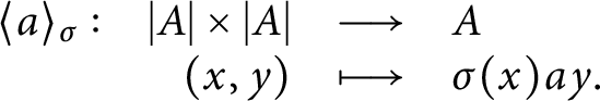 $$ \begin{align*} \begin{array}{rrcl} \langle a\rangle_\sigma : & |A|\times |A| & \longrightarrow & A \\ & (x,y) & \longmapsto & \sigma(x)ay. \end{array} \end{align*} $$
We call such a form elementary diagonal. We will write $\langle a_1,\dots ,a_n\rangle _\sigma $
for an orthogonal sum
$\langle a_1,\dots ,a_n\rangle _\sigma $
for an orthogonal sum $\langle a_1\rangle _\sigma \perp \dots \perp \langle a_n\rangle _\sigma $
(where all
$\langle a_1\rangle _\sigma \perp \dots \perp \langle a_n\rangle _\sigma $
(where all $a_i$
are
$a_i$
are $\varepsilon $
-symmetric), and call such a form diagonal.
$\varepsilon $
-symmetric), and call such a form diagonal.
Remark 3.3 Not every form is diagonalizable. In fact, for $(V,h)$
to be diagonalizable, it is clearly necessary that V is a free A-module (which is in this case equivalent to
$(V,h)$
to be diagonalizable, it is clearly necessary that V is a free A-module (which is in this case equivalent to $\dim _K(V)$
being a multiple of
$\dim _K(V)$
being a multiple of $\dim _K(A)$
). It turns out that this condition is actually sufficient, except in the special case where
$\dim _K(A)$
). It turns out that this condition is actually sufficient, except in the special case where $(A,\sigma )=(K,\operatorname {\mathrm {Id}})$
and
$(A,\sigma )=(K,\operatorname {\mathrm {Id}})$
and $\varepsilon =-1$
, which is the only case where
$\varepsilon =-1$
, which is the only case where $h(x,x)=0$
for all
$h(x,x)=0$
for all $x\in V$
.
$x\in V$
.
3.1.3 Hermitian Morita equivalences
If $(V,h)$
is an
$(V,h)$
is an $\varepsilon $
-hermitian module over
$\varepsilon $
-hermitian module over $(A,\sigma )$
, then the adjoint involution
$(A,\sigma )$
, then the adjoint involution $\sigma _h$
on
$\sigma _h$
on $\operatorname {\mathrm {End}}_A(V)$
is defined (see [Reference Knus, Merkurjev, Rost and Tignol15, 4.1]) by the fact that for all
$\operatorname {\mathrm {End}}_A(V)$
is defined (see [Reference Knus, Merkurjev, Rost and Tignol15, 4.1]) by the fact that for all $x,y\in V$
and all
$x,y\in V$
and all $f\in \operatorname {\mathrm {End}}_A(V)$
,
$f\in \operatorname {\mathrm {End}}_A(V)$
,
 $$ \begin{align*} h(f(x),y) = h(x,\sigma_h(f)(y)). \end{align*} $$
If $(A,\sigma )$
and
$(A,\sigma )$
and $(B,\tau )$
are algebras with involution over
$(B,\tau )$
are algebras with involution over $(K,\iota )$
, we say that
$(K,\iota )$
, we say that $(V,h)$
is an
$(V,h)$
is an $\varepsilon $
-hermitian Morita equivalence between
$\varepsilon $
-hermitian Morita equivalence between $(B,\tau )$
and
$(B,\tau )$
and $(A,\sigma )$
, which we write
$(A,\sigma )$
, which we write
 $$ \begin{align*} (B,\tau) \stackrel{(V,h)}{\rightsquigarrow} (A,\sigma), \end{align*} $$
if $B\stackrel {V}{\rightsquigarrow } A$
, h is an
$B\stackrel {V}{\rightsquigarrow } A$
, h is an $\varepsilon $
-hermitian form over
$\varepsilon $
-hermitian form over $(A,\sigma )$
on V, and
$(A,\sigma )$
on V, and $\tau $
corresponds to
$\tau $
corresponds to $\sigma _h$
through the natural isomorphism
$\sigma _h$
through the natural isomorphism $B\simeq \operatorname {\mathrm {End}}_A(V)$
. In particular, any
$B\simeq \operatorname {\mathrm {End}}_A(V)$
. In particular, any $\varepsilon $
-hermitian module
$\varepsilon $
-hermitian module $(V,h)$
over
$(V,h)$
over $(A,\sigma )$
defines an equivalence
$(A,\sigma )$
defines an equivalence $(\operatorname {\mathrm {End}}_A(V),\sigma _h) \stackrel {(V,h)}{\rightsquigarrow } (A,\sigma )$
. An isomorphism of
$(\operatorname {\mathrm {End}}_A(V),\sigma _h) \stackrel {(V,h)}{\rightsquigarrow } (A,\sigma )$
. An isomorphism of $\varepsilon $
-hermitian Morita equivalences is a bimodule isomorphism which is also an isometry.
$\varepsilon $
-hermitian Morita equivalences is a bimodule isomorphism which is also an isometry.
If $B\stackrel {V}{\rightsquigarrow } A$
, then there always exists an
$B\stackrel {V}{\rightsquigarrow } A$
, then there always exists an $\varepsilon $
-hermitian form h on V such that
$\varepsilon $
-hermitian form h on V such that $(B,\tau ) \stackrel {(V,h)}{\rightsquigarrow } (A,\sigma )$
(see [Reference Knus, Merkurjev, Rost and Tignol15, 4.2]). When the involutions are unitary (so
$(B,\tau ) \stackrel {(V,h)}{\rightsquigarrow } (A,\sigma )$
(see [Reference Knus, Merkurjev, Rost and Tignol15, 4.2]). When the involutions are unitary (so $\iota \neq \operatorname {\mathrm {Id}}$
), we can take any
$\iota \neq \operatorname {\mathrm {Id}}$
), we can take any $\varepsilon \in U(K,\iota )$
; when the involutions are of the first kind (so
$\varepsilon \in U(K,\iota )$
; when the involutions are of the first kind (so $\iota =\operatorname {\mathrm {Id}}$
), then we must take
$\iota =\operatorname {\mathrm {Id}}$
), then we must take $\varepsilon =1$
if
$\varepsilon =1$
if $\sigma $
and
$\sigma $
and $\tau $
have the same type (orthogonal or symplectic), and
$\tau $
have the same type (orthogonal or symplectic), and $\varepsilon =-1$
otherwise. Moreover, in any case, if h and
$\varepsilon =-1$
otherwise. Moreover, in any case, if h and $h'$
are two possible choices, then there is
$h'$
are two possible choices, then there is $\lambda \in K^\times $
such that
$\lambda \in K^\times $
such that $h'=\langle \lambda \rangle h$
.
$h'=\langle \lambda \rangle h$
.
Example 3.4 If $a\in \operatorname {\mathrm {Sym}}^\varepsilon (A^\times , \sigma )$
, then
$a\in \operatorname {\mathrm {Sym}}^\varepsilon (A^\times , \sigma )$
, then $(A,\sigma _a)\stackrel {(|A|,\langle a\rangle _\sigma )}{\rightsquigarrow } (A,\sigma )$
, where
$(A,\sigma _a)\stackrel {(|A|,\langle a\rangle _\sigma )}{\rightsquigarrow } (A,\sigma )$
, where $\sigma _a(x) = a^{-1}\sigma (x)a$
. In particular, if
$\sigma _a(x) = a^{-1}\sigma (x)a$
. In particular, if $a\in K^\times $
, then
$a\in K^\times $
, then $\sigma _a=\sigma $
.
$\sigma _a=\sigma $
.
Example 3.5 Using the involution $\sigma $
on A, we can twist the usual sandwich map (3.1) to
$\sigma $
on A, we can twist the usual sandwich map (3.1) to
 $$ \begin{align} \begin{array}{rcl} A\otimes_K A^{\iota} & \longrightarrow & \operatorname{\mathrm{End}}_K(|A|) \\ a\otimes b & \longmapsto & (x\mapsto ax\sigma(b)), \end{array} \end{align} $$
where $A^{\iota }$
is the same ring as A, but with the twisted K-algebra structure
$A^{\iota }$
is the same ring as A, but with the twisted K-algebra structure $K\xrightarrow {\iota } K\to A$
.
$K\xrightarrow {\iota } K\to A$
.
We call this action of $A\otimes _K A^{\iota }$
on
$A\otimes _K A^{\iota }$
on $|A|$
the “twisted sandwich action” (relative to
$|A|$
the “twisted sandwich action” (relative to $\sigma $
). We will write
$\sigma $
). We will write $|A|_\sigma $
instead of
$|A|_\sigma $
instead of $|A|$
when we see it as a left
$|A|$
when we see it as a left $A\otimes _K A^{\iota }$
-module with this action. It is shown in [Reference Knus, Merkurjev, Rost and Tignol15, 11.1] that the so-called involution trace form
$A\otimes _K A^{\iota }$
-module with this action. It is shown in [Reference Knus, Merkurjev, Rost and Tignol15, 11.1] that the so-called involution trace form
 $$ \begin{align} \begin{array}{rrcl} T_\sigma : & |A|\times |A| & \longrightarrow & K \\ & (x,y) & \longmapsto & \operatorname{\mathrm{Trd}}_A(\sigma(x)y) \end{array} \end{align} $$
is a hermitian form over $(K,\iota )$
on the K-vector space
$(K,\iota )$
on the K-vector space $|A|$
, such that
$|A|$
, such that
 $$ \begin{align} (A\otimes_K A^{\iota},\sigma\otimes \sigma) \stackrel{(|A|_\sigma,T_\sigma)}{\rightsquigarrow} (K,\iota). \end{align} $$
3.1.4 Tensor products
If $(V_i,h_i)$
is an
$(V_i,h_i)$
is an $\varepsilon _i$
-hermitian module over an algebra with involution
$\varepsilon _i$
-hermitian module over an algebra with involution $(A_i,\sigma _i)$
, for
$(A_i,\sigma _i)$
, for $i=1,2$
, then
$i=1,2$
, then $(V_1\otimes _K V_2,h_1\otimes h_2)$
is an
$(V_1\otimes _K V_2,h_1\otimes h_2)$
is an $\varepsilon _1\varepsilon _2$
-hermitian module over (
$\varepsilon _1\varepsilon _2$
-hermitian module over ( $A_1\otimes _K A_2$
,
$A_1\otimes _K A_2$
, $\sigma _1\otimes \sigma _2$
). In particular,
$\sigma _1\otimes \sigma _2$
). In particular, $\langle a\rangle _{\sigma _1}\otimes \langle b\rangle _{\sigma _2}\simeq \langle a\otimes b\rangle _{\sigma _1\otimes \sigma _2}$
.
$\langle a\rangle _{\sigma _1}\otimes \langle b\rangle _{\sigma _2}\simeq \langle a\otimes b\rangle _{\sigma _1\otimes \sigma _2}$
.
If, for $i=1,2$
, we have
$i=1,2$
, we have $(B_i,\tau _i) \stackrel {(V_i,h_i)}{\rightsquigarrow } (A_i,\sigma _i)$
, then
$(B_i,\tau _i) \stackrel {(V_i,h_i)}{\rightsquigarrow } (A_i,\sigma _i)$
, then
 $$ \begin{align*} (B_1\otimes_K B_2,\tau_1\otimes\tau_2) \stackrel{(V_1\otimes_K V_2,h_1\otimes h_2)}{\rightsquigarrow} (A_1\otimes_K A_2,\sigma_1\otimes\sigma_2). \end{align*} $$
3.1.5 Conjugate form
If $(B,\tau ) \stackrel {(V,h)}{\rightsquigarrow } (A,\sigma )$
, then we define
$(B,\tau ) \stackrel {(V,h)}{\rightsquigarrow } (A,\sigma )$
, then we define $(\overline {V},\overline {h})$
, where
$(\overline {V},\overline {h})$
, where $\overline {V}$
is the A–B-bimodule defined as V as a K-vector space, with the action
$\overline {V}$
is the A–B-bimodule defined as V as a K-vector space, with the action
 $$ \begin{align*} a\cdot v\cdot b = \tau(b)\cdot v\cdot \sigma(a), \end{align*} $$
and $\overline {h}: \overline {V}\times \overline {V}\to B$
is characterized by
$\overline {h}: \overline {V}\times \overline {V}\to B$
is characterized by
 $$ \begin{align*} \overline{h}(x,y)z = xh(y,z), \end{align*} $$
for all $x,y,z\in V$
.
$x,y,z\in V$
.
Then it is easy to see that $(A,\sigma ) \stackrel {(\overline {V},\overline {h})}{\rightsquigarrow } (B,\tau )$
.
$(A,\sigma ) \stackrel {(\overline {V},\overline {h})}{\rightsquigarrow } (B,\tau )$
.
3.2 The category
$\mathbf {Br}_h(K,\iota )$

We now define a category $\mathbf {Br}_h(K,\iota )$
, which we call the hermitian Brauer 2-group of
$\mathbf {Br}_h(K,\iota )$
, which we call the hermitian Brauer 2-group of $(K,\iota )$
, such that:
$(K,\iota )$
, such that:
-
• the objects are the algebras with involution
$(A,\sigma )$
over
$(K,\iota )$
and -
• the morphisms from
$(B,\tau )$
to
$(A,\sigma )$
are the isomorphism classes of
$\varepsilon $
-hermitian Morita equivalences between
$(B,\tau ) \stackrel {(V,h)}{\rightsquigarrow } (A,\sigma )$
.


We will usually identify an $\varepsilon $
-hermitian bimodule and its isomorphism class when no confusion is possible. If
$\varepsilon $
-hermitian bimodule and its isomorphism class when no confusion is possible. If $f:(B,\tau )\to (A,\sigma )$
is a morphism in
$f:(B,\tau )\to (A,\sigma )$
is a morphism in $\mathbf {Br}_h(K,\iota )$
, we will sometimes write
$\mathbf {Br}_h(K,\iota )$
, we will sometimes write $(V_f,h_f)$
for the corresponding
$(V_f,h_f)$
for the corresponding $\varepsilon $
-hermitian bimodule. We usually write
$\varepsilon $
-hermitian bimodule. We usually write $\mathbf {Br}_h(K)$
for
$\mathbf {Br}_h(K)$
for $\mathbf {Br}_h(K,\operatorname {\mathrm {Id}})$
.
$\mathbf {Br}_h(K,\operatorname {\mathrm {Id}})$
.
To properly define $\mathbf {Br}_h(K,\iota )$
as a category, we need to specify how to compose morphisms. Given two morphisms
$\mathbf {Br}_h(K,\iota )$
as a category, we need to specify how to compose morphisms. Given two morphisms $(C,\theta )\stackrel {(U,h)}{\rightsquigarrow } (B,\tau )$
and
$(C,\theta )\stackrel {(U,h)}{\rightsquigarrow } (B,\tau )$
and $(B,\tau ) \stackrel {(V,h')}{\rightsquigarrow } (A,\sigma )$
, we define a C–A-bimodule
$(B,\tau ) \stackrel {(V,h')}{\rightsquigarrow } (A,\sigma )$
, we define a C–A-bimodule $V\circ U = U\otimes _B V$
, and a map
$V\circ U = U\otimes _B V$
, and a map $h'\circ h: (V\circ U)\times (V\circ U) \to A$
by
$h'\circ h: (V\circ U)\times (V\circ U) \to A$
by
 $$ \begin{align} (h'\circ h)(u\otimes v, u'\otimes v') = h'(v, h(u,u')v'). \end{align} $$
Proposition 3.6 In the situation just above, if h and $h'$
are, respectively,
$h'$
are, respectively, $\varepsilon $
and
$\varepsilon $
and $\varepsilon '$
-hermitian, then
$\varepsilon '$
-hermitian, then $h'\circ h$
is an
$h'\circ h$
is an $\varepsilon \varepsilon '$
-hermitian form over
$\varepsilon \varepsilon '$
-hermitian form over $(A,\sigma )$
, which defines an equivalence
$(A,\sigma )$
, which defines an equivalence
 $$ \begin{align*} (C,\theta) \stackrel{(V\circ U,h'\circ h)}{\rightsquigarrow} (A,\sigma) \end{align*} $$
whose isomorphism class depends only on the isomorphism classes of $(U,h)$
and
$(U,h)$
and $(V,h')$
.
$(V,h')$
.
Proof This is a reformulation of [Reference Knus14, I.8.1] in the special case of central simple algebras.▪
Example 3.7 Let $f: (B,\tau )\stackrel {(V,h)}{\rightsquigarrow } (A,\sigma )$
be a morphism in
$f: (B,\tau )\stackrel {(V,h)}{\rightsquigarrow } (A,\sigma )$
be a morphism in $\mathbf {Br}_h(K,\iota )$
, and let
$\mathbf {Br}_h(K,\iota )$
, and let $b\in \operatorname {\mathrm {Sym}}^\varepsilon (B^\times , \tau )$
and
$b\in \operatorname {\mathrm {Sym}}^\varepsilon (B^\times , \tau )$
and $a\in \operatorname {\mathrm {Sym}}^{\varepsilon '}(A^\times , \sigma )$
. Then the underlying space of
$a\in \operatorname {\mathrm {Sym}}^{\varepsilon '}(A^\times , \sigma )$
. Then the underlying space of $\langle a\rangle _\sigma \circ f\circ \langle b\rangle _\tau $
is
$\langle a\rangle _\sigma \circ f\circ \langle b\rangle _\tau $
is $|B|\otimes _B V\otimes _A |A|$
, which is canonically identified with V, and the
$|B|\otimes _B V\otimes _A |A|$
, which is canonically identified with V, and the $\varepsilon \varepsilon _f\varepsilon '$
-hermitian form is:
$\varepsilon \varepsilon _f\varepsilon '$
-hermitian form is:
 $$ \begin{align*} \begin{array}{rcl} V\times V & \longrightarrow & A \\ (x,y) & \longmapsto & h(xa,by). \end{array} \end{align*} $$
In particular, $f\circ \langle 1\rangle _\tau = \langle 1\rangle _\sigma \circ f = f$
.
$f\circ \langle 1\rangle _\tau = \langle 1\rangle _\sigma \circ f = f$
.
We can then state the following proposition.
Proposition 3.8 With the composition of morphisms being given by (
3.5
), $\mathbf {Br}_h(K,\iota )$
is a category, and the identity of
$\mathbf {Br}_h(K,\iota )$
is a category, and the identity of $(A,\sigma )$
is
$(A,\sigma )$
is $(|A|,\langle 1\rangle _\sigma )$
. Moreover,
$(|A|,\langle 1\rangle _\sigma )$
. Moreover, $\mathbf {Br}_h(K,\iota )$
is actually a groupoid, and the inverse of a morphism
$\mathbf {Br}_h(K,\iota )$
is actually a groupoid, and the inverse of a morphism $(V,h)$
is
$(V,h)$
is $(\overline {V},\varepsilon _h\overline {h})$
.
$(\overline {V},\varepsilon _h\overline {h})$
.
Proof All statements are rephrasings of classical statements in hermitian Morita theory, in the special case of central simple algebras with involution of the first kind. The associativity of the composition is proved in [Reference Knus14, I.8.1.1]. The statement on identities follows from Example 3.7, and the statement about inverses is proved in [Reference Knus14, I.9.3.4].▪
3.3 Automorphisms and isometries
We defined a category $\mathbf {Br}_h(K,\iota )$
in which the (iso)morphisms between two algebras with involution correspond to hermitian Morita equivalences. However, obviously, there is a more elementary notion of isomorphism between algebras with involution. To be precise, we may define a category
$\mathbf {Br}_h(K,\iota )$
in which the (iso)morphisms between two algebras with involution correspond to hermitian Morita equivalences. However, obviously, there is a more elementary notion of isomorphism between algebras with involution. To be precise, we may define a category $\mathbf {AlgInv}(K,\iota )$
, with the same objects as
$\mathbf {AlgInv}(K,\iota )$
, with the same objects as $\mathbf {Br}_h(K,\iota )$
, but where the morphisms are K-algebra isomorphisms which are compatible with the involutions.
$\mathbf {Br}_h(K,\iota )$
, but where the morphisms are K-algebra isomorphisms which are compatible with the involutions.
Then, to any algebra isomorphism $\varphi : (B,\tau )\to (A,\sigma )$
, we can associate
$\varphi : (B,\tau )\to (A,\sigma )$
, we can associate $(B,\tau ) \stackrel {(|A|_\varphi ,\langle 1\rangle _\sigma )}{\rightsquigarrow } (A,\sigma )$
where
$(B,\tau ) \stackrel {(|A|_\varphi ,\langle 1\rangle _\sigma )}{\rightsquigarrow } (A,\sigma )$
where $|A|_\varphi =|A|$
as a right A-module, and the left action of B is given by
$|A|_\varphi =|A|$
as a right A-module, and the left action of B is given by $b\cdot a = \varphi (b)a$
for any
$b\cdot a = \varphi (b)a$
for any $b\in B$
and
$b\in B$
and $a\in |A|$
. It is easily seen that this is indeed a hermitian Morita equivalence, and that this defines a functor
$a\in |A|$
. It is easily seen that this is indeed a hermitian Morita equivalence, and that this defines a functor
 $$ \begin{align*} \Theta: \mathbf{AlgInv}(K,\iota)\to \mathbf{Br}_h(K,\iota), \end{align*} $$
which is the identity on objects.
Obviously, this functor is far from being full, since there are isomorphisms in $\mathbf {Br}_h(K,\iota )$
between
$\mathbf {Br}_h(K,\iota )$
between $(B,\tau )$
and
$(B,\tau )$
and $(A,\sigma )$
whenever A and B are Brauer-equivalent. On the other hand, we can look at the situation where
$(A,\sigma )$
whenever A and B are Brauer-equivalent. On the other hand, we can look at the situation where $(A,\sigma )=(B,\tau )$
. We call
$(A,\sigma )=(B,\tau )$
. We call
 $$ \begin{align*} \operatorname{\mathrm{Aut}}_{\mathcal{M}}(A,\sigma) := \operatorname{\mathrm{Aut}}_{\mathbf{Br}_h(K,\iota)}(A,\sigma) \end{align*} $$
the group of Morita automorphisms of $(A,\sigma )$
, and
$(A,\sigma )$
, and
 $$ \begin{align*} \operatorname{\mathrm{Aut}}_K(A,\sigma) := \operatorname{\mathrm{Aut}}_{\mathbf{AlgInv}(K,\iota)}(A,\sigma) \end{align*} $$
the group of algebraic automorphisms of $(A,\sigma )$
. By extension, we say that a morphism in
$(A,\sigma )$
. By extension, we say that a morphism in $\mathbf {Br}_h(K,\iota )$
is algebraic if it is in the image of
$\mathbf {Br}_h(K,\iota )$
is algebraic if it is in the image of $\Theta $
. Then we have a group morphism
$\Theta $
. Then we have a group morphism
 $$ \begin{align*} \Theta: \operatorname{\mathrm{Aut}}_K(A,\sigma) \longrightarrow \operatorname{\mathrm{Aut}}_{\mathcal{M}}(A,\sigma), \end{align*} $$
and we want to understand the groups involved, as well as the kernel and cokernel.
Recall from [Reference Knus, Merkurjev, Rost and Tignol15, 12.14] that the subgroup $\operatorname {\mathrm {Sim}}(A,\sigma )\subset A^\times $
of similitudes of
$\operatorname {\mathrm {Sim}}(A,\sigma )\subset A^\times $
of similitudes of $(A,\sigma )$
is defined as
$(A,\sigma )$
is defined as
 $$ \begin{align*} \operatorname{\mathrm{Sim}}(A,\sigma) = \{ a\in A\,|\, a\sigma(a) \in k^\times\}. \end{align*} $$
When $a\in \operatorname {\mathrm {Sim}}(A,\sigma )$
, we can define its multiplier
$a\in \operatorname {\mathrm {Sim}}(A,\sigma )$
, we can define its multiplier $\mu (a)=a\sigma (a)=\sigma (a)a\in k^\times $
, and
$\mu (a)=a\sigma (a)=\sigma (a)a\in k^\times $
, and $\mu $
is a group morphism
$\mu $
is a group morphism $\operatorname {\mathrm {Sim}}(A,\sigma )\to k^\times $
. Then
$\operatorname {\mathrm {Sim}}(A,\sigma )\to k^\times $
. Then $\operatorname {\mathrm {Ker}}(\mu )$
is the subgroup
$\operatorname {\mathrm {Ker}}(\mu )$
is the subgroup $\operatorname {\mathrm {Iso}}(A,\sigma )$
of isometries of
$\operatorname {\mathrm {Iso}}(A,\sigma )$
of isometries of $(A,\sigma )$
, and
$(A,\sigma )$
, and $\operatorname {\mathrm {Im}}(\mu )=G(A,\sigma )$
is the group of multipliers of
$\operatorname {\mathrm {Im}}(\mu )=G(A,\sigma )$
is the group of multipliers of $(A,\sigma )$
. The following proposition gives a complete picture of the situation.
$(A,\sigma )$
. The following proposition gives a complete picture of the situation.
Proposition 3.9 Let $(A,\sigma )$
be an algebra with involution over
$(A,\sigma )$
be an algebra with involution over $(K,\iota )$
. We write
$(K,\iota )$
. We write $N: K^\times \to k^\times $
for the group morphism
$N: K^\times \to k^\times $
for the group morphism $x\mapsto x\iota (x)$
(when
$x\mapsto x\iota (x)$
(when $\iota \neq \operatorname {\mathrm {Id}}$
, this is the Galois norm of
$\iota \neq \operatorname {\mathrm {Id}}$
, this is the Galois norm of $K/k$
), and
$K/k$
), and $\operatorname {\mathrm {int}}(a)\in \operatorname {\mathrm {Aut}}_K(A)$
for the inner automorphism of A induced by some
$\operatorname {\mathrm {int}}(a)\in \operatorname {\mathrm {Aut}}_K(A)$
for the inner automorphism of A induced by some $a\in A^\times $
.
$a\in A^\times $
.
Then we have a commutative diagram of groups with exact rows and columns:

In particular, there is a canonical isomorphism $\operatorname {\mathrm {Aut}}_{\mathcal {M}}(A,\sigma )\simeq K^\times /N(K^\times )$
, and when
$\operatorname {\mathrm {Aut}}_{\mathcal {M}}(A,\sigma )\simeq K^\times /N(K^\times )$
, and when $\iota =\operatorname {\mathrm {Id}}$
, this gives
$\iota =\operatorname {\mathrm {Id}}$
, this gives $\operatorname {\mathrm {Aut}}_{\mathcal {M}}(A,\sigma )\simeq K^\times /K^{\times 2}$
.
$\operatorname {\mathrm {Aut}}_{\mathcal {M}}(A,\sigma )\simeq K^\times /K^{\times 2}$
.
Proof To prove that the diagram commutes, the only nontrivial thing to show is that for any $a\in \operatorname {\mathrm {Sim}}(A,\sigma )$
,
$a\in \operatorname {\mathrm {Sim}}(A,\sigma )$
, $\Theta (\operatorname {\mathrm {int}}(a)) \simeq (|A|, \langle \mu (a)\rangle _\sigma )$
. By definition,
$\Theta (\operatorname {\mathrm {int}}(a)) \simeq (|A|, \langle \mu (a)\rangle _\sigma )$
. By definition, $\Theta (\operatorname {\mathrm {int}}(a))$
corresponds to the hermitian A–A-bimodule
$\Theta (\operatorname {\mathrm {int}}(a))$
corresponds to the hermitian A–A-bimodule $(|A|_a,\langle 1\rangle _\sigma )$
, where
$(|A|_a,\langle 1\rangle _\sigma )$
, where $|A|_a=|A|$
as a right A-module, and the action on the left is given by
$|A|_a=|A|$
as a right A-module, and the action on the left is given by $x\cdot y = axa^{-1}y$
for all
$x\cdot y = axa^{-1}y$
for all $x\in A$
,
$x\in A$
, $y\in |A|_a$
. Then we easily see that
$y\in |A|_a$
. Then we easily see that
 $$ \begin{align*} \begin{array}{rrcl} f : & |A|_a & \longrightarrow & |A| \\ & y & \longmapsto & a^{-1}y \end{array} \end{align*} $$
is a bimodule isomorphism. Since
 $$ \begin{align*} \langle \mu(a)\rangle_\sigma(f(x),f(y)) = \mu(a)\sigma(f(x))f(y) = \mu(a)\sigma(x)\sigma(a)^{-1}a^{-1}y=\sigma(x)y, \end{align*} $$
the map f induces an isometry from $\langle 1\rangle _\sigma $
to
$\langle 1\rangle _\sigma $
to $\langle \mu (a)\rangle _\sigma $
, which shows that the diagram commutes.
$\langle \mu (a)\rangle _\sigma $
, which shows that the diagram commutes.
The exactness of each row is clear. The exactness of the second column is a consequence of [Reference Knus, Merkurjev, Rost and Tignol15, 12.15]. For the third column, the surjectivity comes from the fact that any automorphism of $(A,\sigma )$
in
$(A,\sigma )$
in $\mathbf {Br}_h(K,\iota )$
has the form
$\mathbf {Br}_h(K,\iota )$
has the form $(|A|,h)$
, and since
$(|A|,h)$
, and since $h=\langle 1\rangle _\sigma $
is a possible choice, any other choice must have the form
$h=\langle 1\rangle _\sigma $
is a possible choice, any other choice must have the form $h=\langle \lambda \rangle _\sigma $
. To prove exactness at
$h=\langle \lambda \rangle _\sigma $
. To prove exactness at $K^\times $
, we must also show that
$K^\times $
, we must also show that $(|A|,\langle \lambda \rangle _\sigma )$
and
$(|A|,\langle \lambda \rangle _\sigma )$
and $(|A|,\langle 1\rangle _\sigma )$
are isomorphic iff
$(|A|,\langle 1\rangle _\sigma )$
are isomorphic iff $\lambda \in N(K^\times )$
. However, any bimodule isomorphism
$\lambda \in N(K^\times )$
. However, any bimodule isomorphism $f:|A|\to |A|$
has the form
$f:|A|\to |A|$
has the form $f(x)=ax$
for some
$f(x)=ax$
for some $a\in K^\times $
, so if it induces an isometry from
$a\in K^\times $
, so if it induces an isometry from $\langle \lambda \rangle _\sigma $
to
$\langle \lambda \rangle _\sigma $
to $\langle 1\rangle _\sigma $
, we must have
$\langle 1\rangle _\sigma $
, we must have $\lambda =a\iota (a)$
.
$\lambda =a\iota (a)$
.
For the first and fourth columns, the only thing to show is the surjectivity, but it is easily obtained by a diagram chase now that we have shown exactness everywhere else.▪
Remark 3.10 Given two morphisms $f_i: (B_i,\tau _i)\stackrel {(V_i,h_i)}{\rightsquigarrow } (A,\sigma )$
in
$f_i: (B_i,\tau _i)\stackrel {(V_i,h_i)}{\rightsquigarrow } (A,\sigma )$
in $\mathbf {Br}_h(K,\iota )$
, since
$\mathbf {Br}_h(K,\iota )$
, since $\mathbf {Br}_h(K,\iota )$
is a groupoid, there is a unique
$\mathbf {Br}_h(K,\iota )$
is a groupoid, there is a unique $g: (B_1,\tau _1)\to (B_2,\tau _2)$
such that
$g: (B_1,\tau _1)\to (B_2,\tau _2)$
such that $f_1 = f_2\circ g$
. Now,
$f_1 = f_2\circ g$
. Now, $h_i$
is isometric to
$h_i$
is isometric to $h_2$
if and only if g is algebraic. Thus,
$h_2$
if and only if g is algebraic. Thus, $\mathbf {Br}_h(K,\iota )$
cannot detect isometric modules on its own, but it can if we add the data of
$\mathbf {Br}_h(K,\iota )$
cannot detect isometric modules on its own, but it can if we add the data of $\Theta $
.
$\Theta $
.
3.4 Monoidal structure and the Goldman element
The tensor product of algebras with involution endows $\mathbf {AlgInv}(K,\iota )$
with a natural symmetric monoidal structure, with unit object
$\mathbf {AlgInv}(K,\iota )$
with a natural symmetric monoidal structure, with unit object $(K,\iota )$
, such that the obvious forgetful functor
$(K,\iota )$
, such that the obvious forgetful functor $\mathbf {AlgInv}(K,\iota )\to K\text {-}\mathbf {Alg}$
(which is faithful but not full) is symmetric strong monoidal.
$\mathbf {AlgInv}(K,\iota )\to K\text {-}\mathbf {Alg}$
(which is faithful but not full) is symmetric strong monoidal.
Likewise, the tensor product of algebras with involution (and of hermitian modules, for the morphisms) defines a monoidal structure on $\mathbf {Br}_h(K,\iota )$
, with unit object
$\mathbf {Br}_h(K,\iota )$
, with unit object $(K,\iota )$
, such that
$(K,\iota )$
, such that $\Theta : \mathbf {AlgInv}(K,\iota )\to \mathbf {Br}_h(K,\iota )$
is a strict monoidal functor. We can also transport the symmetric structure.
$\Theta : \mathbf {AlgInv}(K,\iota )\to \mathbf {Br}_h(K,\iota )$
is a strict monoidal functor. We can also transport the symmetric structure.
Proposition 3.11 The monoidal category $\mathbf {Br}_h(K,\iota )$
has a unique symmetric structure such that
$\mathbf {Br}_h(K,\iota )$
has a unique symmetric structure such that $\Theta $
is symmetric.
$\Theta $
is symmetric.
Proof If we want $\Theta $
to be symmetric, we need to define the switching map in
$\Theta $
to be symmetric, we need to define the switching map in $\mathbf {Br}_h(K,\iota )$
as
$\mathbf {Br}_h(K,\iota )$
as
 $$ \begin{align*} (A,\sigma)\otimes_K (B,\tau) \xrightarrow{\Theta(s)} (B,\tau)\otimes_K (A,\sigma), \end{align*} $$
where $s: (A,\sigma )\otimes _K (B,\tau )\to (B,\tau )\otimes _K (A,\sigma )$
is the switching map in
$s: (A,\sigma )\otimes _K (B,\tau )\to (B,\tau )\otimes _K (A,\sigma )$
is the switching map in $\mathbf {AlgInv}(K,\iota )$
.
$\mathbf {AlgInv}(K,\iota )$
.
Since the switching maps, the associators, and the unit maps are all images of morphisms in $\mathbf {AlgInv}(K,\iota )$
by
$\mathbf {AlgInv}(K,\iota )$
by $\Theta $
, all the coherence axioms can be verified in
$\Theta $
, all the coherence axioms can be verified in $\mathbf {AlgInv}(K,\iota )$
.▪
$\mathbf {AlgInv}(K,\iota )$
.▪
In particular, this means that for any algebra with involution $(A,\sigma )$
over
$(A,\sigma )$
over $(K,\iota )$
and any
$(K,\iota )$
and any $n\in \mathbb {N}$
, there are natural group morphisms
$n\in \mathbb {N}$
, there are natural group morphisms

A remarkable feature of Azumaya algebras is the existence of the so-called Goldman element (see [Reference Knus, Merkurjev, Rost and Tignol15, 3.A]).
Definition 3.1 Let A be a central simple algebra over K. Its Goldman element $g_A\in A\otimes _K A$
is defined by the fact that the sandwich map (3.1) sends
$g_A\in A\otimes _K A$
is defined by the fact that the sandwich map (3.1) sends $g_A$
, seen as an element of
$g_A$
, seen as an element of $A\otimes _K A^{op}$
, to the reduced trace
$A\otimes _K A^{op}$
, to the reduced trace $\operatorname {\mathrm {Trd}}_A: A\to K$
, viewed as a linear map
$\operatorname {\mathrm {Trd}}_A: A\to K$
, viewed as a linear map $|A|\to |A|$
.
$|A|\to |A|$
.
It is shown in [Reference Knus, Merkurjev, Rost and Tignol15, 10.1] that the natural morphism $\mathfrak {S}_n\to \operatorname {\mathrm {Aut}}_K(A^{\otimes n})$
admits a lift
$\mathfrak {S}_n\to \operatorname {\mathrm {Aut}}_K(A^{\otimes n})$
admits a lift
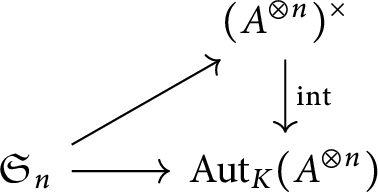
where $\mathfrak {S}_n\to (A^{\otimes n})^\times $
is uniquely characterized by
$\mathfrak {S}_n\to (A^{\otimes n})^\times $
is uniquely characterized by
 $$ \begin{align*} (i, i+1) \mapsto 1\otimes\cdots \otimes g_A \otimes 1\otimes \dots \otimes 1 \end{align*} $$
(with $g_A$
occupying the i and
$g_A$
occupying the i and $i+1$
slots).
$i+1$
slots).
Proposition 3.12 Let $(A,\sigma )$
be an algebra with involution over
$(A,\sigma )$
be an algebra with involution over $(K,\iota )$
. Then the natural morphism
$(K,\iota )$
. Then the natural morphism $\mathfrak {S}_n\to (A^{\otimes n})^\times $
gives a commutative diagram of groups:
$\mathfrak {S}_n\to (A^{\otimes n})^\times $
gives a commutative diagram of groups:

Proof The only thing to show is that $\mathfrak {S}_n\to (A^{\otimes n})^\times $
actually takes values in
$\mathfrak {S}_n\to (A^{\otimes n})^\times $
actually takes values in $\operatorname {\mathrm {Iso}}(A^{\otimes n},\sigma ^{\otimes n})$
. It is enough to consider transpositions of the form
$\operatorname {\mathrm {Iso}}(A^{\otimes n},\sigma ^{\otimes n})$
. It is enough to consider transpositions of the form $(i,i+1)$
, which means that it is enough to show that
$(i,i+1)$
, which means that it is enough to show that $g_A\in \operatorname {\mathrm {Iso}}(A^{\otimes 2},\sigma ^{\otimes 2})$
. Since
$g_A\in \operatorname {\mathrm {Iso}}(A^{\otimes 2},\sigma ^{\otimes 2})$
. Since $g_A^2=1$
[Reference Knus, Merkurjev, Rost and Tignol15, 3.6], this is the same as proving that
$g_A^2=1$
[Reference Knus, Merkurjev, Rost and Tignol15, 3.6], this is the same as proving that $g_A$
is symmetric for
$g_A$
is symmetric for $\sigma \otimes \sigma $
, which is proved in [Reference Knus, Merkurjev, Rost and Tignol15, 10.19].▪
$\sigma \otimes \sigma $
, which is proved in [Reference Knus, Merkurjev, Rost and Tignol15, 10.19].▪
The crucial consequence is the following.
Corollary 3.13 The symmetric monoidal category $\mathbf {Br}_h(K,\iota )$
is strongly symmetric.
$\mathbf {Br}_h(K,\iota )$
is strongly symmetric.


3.5 Inverses and coherent
$2$
-torsion

For any small category C, let us write $\pi _0(C)$
for its set of isomorphism classes. When C is monoidal,
$\pi _0(C)$
for its set of isomorphism classes. When C is monoidal, $\pi _0(C)$
inherits a natural monoid structure, which is commutative when
$\pi _0(C)$
inherits a natural monoid structure, which is commutative when $\mathbf {C}$
is symmetric. As we have already stated, there is a morphism in
$\mathbf {C}$
is symmetric. As we have already stated, there is a morphism in $\mathbf {Br}_h(K,\iota )$
between
$\mathbf {Br}_h(K,\iota )$
between $(B,\tau )$
and
$(B,\tau )$
and $(A,\sigma )$
if and only if A and B are Brauer-equivalent, which means that we get a canonical embedding
$(A,\sigma )$
if and only if A and B are Brauer-equivalent, which means that we get a canonical embedding $\pi _0(\mathbf {Br}_h(K,\iota ))\to \operatorname {\mathrm {Br}}(K)$
. In particular, all objects in
$\pi _0(\mathbf {Br}_h(K,\iota ))\to \operatorname {\mathrm {Br}}(K)$
. In particular, all objects in $\mathbf {Br}_h(K,\iota )$
are weakly invertible. When
$\mathbf {Br}_h(K,\iota )$
are weakly invertible. When $\iota \neq \operatorname {\mathrm {Id}}$
,
$\iota \neq \operatorname {\mathrm {Id}}$
, $\pi _0(\mathbf {Br}_h(K,\iota ))$
is identified with the kernel of the norm map
$\pi _0(\mathbf {Br}_h(K,\iota ))$
is identified with the kernel of the norm map $\operatorname {\mathrm {Br}}(K)\to \operatorname {\mathrm {Br}}(k)$
; when
$\operatorname {\mathrm {Br}}(K)\to \operatorname {\mathrm {Br}}(k)$
; when $\iota =\operatorname {\mathrm {Id}}$
,
$\iota =\operatorname {\mathrm {Id}}$
, $\pi _0(\mathbf {Br}_h(K))$
is identified with the
$\pi _0(\mathbf {Br}_h(K))$
is identified with the $2$
-torsion subgroup
$2$
-torsion subgroup $\operatorname {\mathrm {Br}}(K)[2]$
(in particular, every object has weak
$\operatorname {\mathrm {Br}}(K)[2]$
(in particular, every object has weak $2$
-torsion).
$2$
-torsion).
In fact, Example 3.5 gives a more precise statement about invertibility and torsion, as it gives an explicit weak inverse of each $(A,\sigma )$
, namely
$(A,\sigma )$
, namely $(A^{\iota },\sigma )$
, which is indeed equal to
$(A^{\iota },\sigma )$
, which is indeed equal to $(A,\sigma )$
when
$(A,\sigma )$
when $\iota =\operatorname {\mathrm {Id}}$
, and an explicit equivalence from their product to the unit object
$\iota =\operatorname {\mathrm {Id}}$
, and an explicit equivalence from their product to the unit object $(K,\iota )$
, given by the involution trace form
$(K,\iota )$
, given by the involution trace form $(|A|_\sigma ,T_\sigma )$
.
$(|A|_\sigma ,T_\sigma )$
.
According to Theorem 2.16, since $\mathbf {Br}_h(K,\iota )$
is strongly symmetric by Corollary 3.13, the data of all those equivalences define a canonical abelian gs-structure
$\mathbf {Br}_h(K,\iota )$
is strongly symmetric by Corollary 3.13, the data of all those equivalences define a canonical abelian gs-structure $\mathbf {Br}_h(K,\iota ) \to \mathbf {Br}_h(K,\iota )^{\times ,s}$
. This is always the one we implicitly refer to when we mention such a structure.
$\mathbf {Br}_h(K,\iota ) \to \mathbf {Br}_h(K,\iota )^{\times ,s}$
. This is always the one we implicitly refer to when we mention such a structure.
When $\iota =\operatorname {\mathrm {Id}}$
, we can hope to give
$\iota =\operatorname {\mathrm {Id}}$
, we can hope to give $\mathbf {Br}_h(K,\iota )$
a coherent
$\mathbf {Br}_h(K,\iota )$
a coherent $2$
-torsion structure since all objects have weak
$2$
-torsion structure since all objects have weak $2$
-torsion, and indeed:
$2$
-torsion, and indeed:
Theorem 3.14 Associating to each $(A,\sigma )\in \mathbf {Br}_h(K)$
, the canonical equivalence
$(A,\sigma )\in \mathbf {Br}_h(K)$
, the canonical equivalence $(A\otimes _K A,\sigma \otimes \sigma )\stackrel {(|A|_\sigma ,T_\sigma )}{\rightsquigarrow } (K,\operatorname {\mathrm {Id}})$
defines, in the way of Proposition 2.17, a canonical coherent
$(A\otimes _K A,\sigma \otimes \sigma )\stackrel {(|A|_\sigma ,T_\sigma )}{\rightsquigarrow } (K,\operatorname {\mathrm {Id}})$
defines, in the way of Proposition 2.17, a canonical coherent $2$
-torsion structure on
$2$
-torsion structure on $\mathbf {Br}_h(K)$
.
$\mathbf {Br}_h(K)$
.
Proof According to Proposition 2.17, we have to verify the two diagrams (2.6) and (2.7). The first one is straightforward, using the fact that the reduced trace $\operatorname {\mathrm {Trd}}_{A\otimes _K B}$
of
$\operatorname {\mathrm {Trd}}_{A\otimes _K B}$
of $A\otimes _K B$
is nothing but
$A\otimes _K B$
is nothing but $\operatorname {\mathrm {Trd}}_A\otimes \operatorname {\mathrm {Trd}}_B$
.
$\operatorname {\mathrm {Trd}}_A\otimes \operatorname {\mathrm {Trd}}_B$
.
The second one requires more work; it states that for any $f:(B,\tau )\stackrel {(V,h)}{\rightsquigarrow } (A,\sigma )$
in
$f:(B,\tau )\stackrel {(V,h)}{\rightsquigarrow } (A,\sigma )$
in $\mathbf {Br}_h(K)$
, the diagram
$\mathbf {Br}_h(K)$
, the diagram

commutes. We define the following $(B\otimes _K B)$
–K-bimodule morphism:
$(B\otimes _K B)$
–K-bimodule morphism:
 $$ \begin{align*} \begin{array}{rrcl} \psi : & (V\otimes_K V)\otimes_{A\otimes_K A}A & \longrightarrow & B \\ & {(v\otimes w)\otimes a} & \longmapsto &{\varphi_h(va\otimes w),} \end{array} \end{align*} $$
where $\varphi _h: V\otimes _K V\to B$
(see [Reference Knus, Merkurjev, Rost and Tignol15, 5.1]) is given, identifying
$\varphi _h: V\otimes _K V\to B$
(see [Reference Knus, Merkurjev, Rost and Tignol15, 5.1]) is given, identifying $B=\operatorname {\mathrm {End}}_A(V)$
, by
$B=\operatorname {\mathrm {End}}_A(V)$
, by
 $$ \begin{align*} \varphi_h(v\otimes w)(x) = vh(w,x). \end{align*} $$
Then $\psi $
is well defined since for
$\psi $
is well defined since for $x,y\in A$
:
$x,y\in A$
:
 $$ \begin{align*} \psi((v\otimes w)\otimes (xa\sigma(y)) &= \varphi_h(vxa\sigma(y)\otimes w) \\ &= \varphi_h(vxa\otimes wy) \\ &= \psi ((vx\otimes wy)\otimes a), \end{align*} $$
and it is a bimodule morphism since for $x,y\in B$
:
$x,y\in B$
:
 $$ \begin{align*} \psi((xv\otimes yw)\otimes a) &= \varphi_h(xva\otimes yw) \\ &= x\varphi_h(va\otimes v)\tau(y). \end{align*} $$
To show that $\psi $
is an isometry, we must establish equality between on the one hand
$\psi $
is an isometry, we must establish equality between on the one hand
 $$ \begin{align*} & \operatorname{\mathrm{Trd}}_B\left(\tau \left( \psi((v\otimes w)\otimes a)\right)\cdot \psi(((v'\otimes w')\otimes b))\right) \\ &= \operatorname{\mathrm{Trd}}_B\left( \tau(\varphi_h(va\otimes w))\cdot \varphi_h(v'b\otimes w')\right) \end{align*} $$
and on the other hand
 $$ \begin{align*} & \operatorname{\mathrm{Trd}}_A \left(\sigma(a)(h\otimes h)(v\otimes w,v'\otimes w')\cdot b\right) \\ &= \varepsilon \operatorname{\mathrm{Trd}}_A(\sigma(a)h(v,v')bh(w',w)) \end{align*} $$
with $\varepsilon =\varepsilon _h$
. Now, applying successively the formulas in theorem [Reference Knus, Merkurjev, Rost and Tignol15, 5.1], we get:
$\varepsilon =\varepsilon _h$
. Now, applying successively the formulas in theorem [Reference Knus, Merkurjev, Rost and Tignol15, 5.1], we get:
 $$ \begin{align*} & \operatorname{\mathrm{Trd}}_B\left( \tau(\varphi_h(va\otimes w)) \cdot \varphi_h(v'b\otimes w')\right) \\ &= \varepsilon \operatorname{\mathrm{Trd}}_B\left(\varphi_h(w\otimes va) \cdot \varphi_h(v'b\otimes w')\right) \\ &= \varepsilon \operatorname{\mathrm{Trd}}_B\left(\varphi_h( wh(va,v'b) \otimes w') \right) \\ &= \varepsilon \operatorname{\mathrm{Trd}}_A\left(h(w',wh(va,v'b))\right) \\ &= \varepsilon \operatorname{\mathrm{Trd}}_A\left(h(w',w)\sigma(a)h(v,v')b\right)\kern-1pt.\\[-34pt] \end{align*} $$
▪
4 The mixed Witt ring
In this section, we combine the techniques developed in Section 2.4 to define graded rings with the structure on $\mathbf {Br}_h(K,\iota )$
we established in Section 3.5.
$\mathbf {Br}_h(K,\iota )$
we established in Section 3.5.
4.1 The Witt groups
We start by defining the underlying group structures.
Definition 4.1 Let $(A,\sigma )$
be an algebra with involution over
$(A,\sigma )$
be an algebra with involution over $(K,\iota )$
, and let
$(K,\iota )$
, and let $\varepsilon \in U(K,\iota )$
. We denote by
$\varepsilon \in U(K,\iota )$
. We denote by $SW^\varepsilon (A,\sigma )$
the set of isometry classes of
$SW^\varepsilon (A,\sigma )$
the set of isometry classes of $\varepsilon $
-hermitian modules over
$\varepsilon $
-hermitian modules over $(A,\sigma )$
; it is a commutative semigroup when equipped with the orthogonal direct sum of
$(A,\sigma )$
; it is a commutative semigroup when equipped with the orthogonal direct sum of $\varepsilon $
-hermitian modules.
$\varepsilon $
-hermitian modules.
We define $SW_\varepsilon (A,\sigma )=SW^{t(\sigma )\varepsilon }(A,\sigma )$
where
$SW_\varepsilon (A,\sigma )=SW^{t(\sigma )\varepsilon }(A,\sigma )$
where $t(\sigma )= 1$
when
$t(\sigma )= 1$
when $\sigma $
is orthogonal or unitary, and
$\sigma $
is orthogonal or unitary, and $t(\sigma )= -1$
when
$t(\sigma )= -1$
when $\sigma $
is symplectic.
$\sigma $
is symplectic.
We also set: $SW_\pm (A,\sigma ) = SW_1(A,\sigma )\oplus SW_{-1}(A,\sigma )$
.
$SW_\pm (A,\sigma ) = SW_1(A,\sigma )\oplus SW_{-1}(A,\sigma )$
.
We often make the slight abuse of notations $SW_\varepsilon (K)$
for
$SW_\varepsilon (K)$
for $SW_\varepsilon (K,\operatorname {\mathrm {Id}})$
; note that
$SW_\varepsilon (K,\operatorname {\mathrm {Id}})$
; note that $SW_\varepsilon (K)=SW^\varepsilon (K)$
.
$SW_\varepsilon (K)=SW^\varepsilon (K)$
.
We can observe that there is a natural functoriality for those semigroups: if $f: (B,\tau ) \to (A,\sigma )$
is a morphism in
$f: (B,\tau ) \to (A,\sigma )$
is a morphism in $\mathbf {Br}_h(K,\iota )$
with sign
$\mathbf {Br}_h(K,\iota )$
with sign $\varepsilon '\in U(K,\iota )$
, then it induces a function
$\varepsilon '\in U(K,\iota )$
, then it induces a function
 $$ \begin{align} f_*: SW^{\varepsilon}(B,\tau)\longrightarrow SW^{\varepsilon\varepsilon'}(A,\sigma) \end{align} $$
given by $g\mapsto f\circ g$
, where we see any
$g\mapsto f\circ g$
, where we see any $(V,h)\in SW^{\varepsilon }(B,\tau )$
as a morphism
$(V,h)\in SW^{\varepsilon }(B,\tau )$
as a morphism $g: (\operatorname {\mathrm {End}}_K(V),\tau _h)\stackrel {(V,h)}{\rightsquigarrow } (B,\tau )$
.
$g: (\operatorname {\mathrm {End}}_K(V),\tau _h)\stackrel {(V,h)}{\rightsquigarrow } (B,\tau )$
.
To simplify things a bit, and with no real consequence to the theory, we are going to consider the subcategory $\mathbf {Br}_h(K,\iota )'$
of
$\mathbf {Br}_h(K,\iota )'$
of $\mathbf {Br}_h(K,\iota )$
, which is equal to
$\mathbf {Br}_h(K,\iota )$
, which is equal to $\mathbf {Br}_h(K,\iota )$
when
$\mathbf {Br}_h(K,\iota )$
when $\iota =\operatorname {\mathrm {Id}}$
, but only includes the morphisms which are
$\iota =\operatorname {\mathrm {Id}}$
, but only includes the morphisms which are $1$
-hermitian when
$1$
-hermitian when $\iota \neq \operatorname {\mathrm {Id}}$
. The restriction is mostly harmless, since any two objects which are isomorphic in
$\iota \neq \operatorname {\mathrm {Id}}$
. The restriction is mostly harmless, since any two objects which are isomorphic in $\mathbf {Br}_h(K,\iota )$
are still isomorphic in
$\mathbf {Br}_h(K,\iota )$
are still isomorphic in $\mathbf {Br}_h(K,\iota )'$
.
$\mathbf {Br}_h(K,\iota )'$
.
Proposition 4.1 For any $\varepsilon \in U(K,\iota )$
, the association
$\varepsilon \in U(K,\iota )$
, the association $(A,\sigma )\mapsto SW_\varepsilon (A,\sigma )$
and
$(A,\sigma )\mapsto SW_\varepsilon (A,\sigma )$
and $f\mapsto f_*$
as described above defines a functor from
$f\mapsto f_*$
as described above defines a functor from $\mathbf {Br}_h(K,\iota )'$
to the category of commutative semigroups. In particular, each
$\mathbf {Br}_h(K,\iota )'$
to the category of commutative semigroups. In particular, each $f_*$
is actually an isomorphism.
$f_*$
is actually an isomorphism.
Proof First, we need to establish that $f_*$
does define a function from
$f_*$
does define a function from $SW_\varepsilon (B,\tau )$
to
$SW_\varepsilon (B,\tau )$
to $SW_\varepsilon (A,\sigma )$
. When
$SW_\varepsilon (A,\sigma )$
. When $\iota \neq \operatorname {\mathrm {Id}}$
, this comes from the restriction to
$\iota \neq \operatorname {\mathrm {Id}}$
, this comes from the restriction to $\mathbf {Br}_h(K,\iota )'$
, since in (4.1) we have
$\mathbf {Br}_h(K,\iota )'$
, since in (4.1) we have $\varepsilon '=1$
. When
$\varepsilon '=1$
. When $\iota =\operatorname {\mathrm {Id}}$
, there is no a priori restriction on
$\iota =\operatorname {\mathrm {Id}}$
, there is no a priori restriction on $\varepsilon '$
, but it is actually determined by the types of
$\varepsilon '$
, but it is actually determined by the types of $\sigma $
and
$\sigma $
and $\tau $
. In fact, we get
$\tau $
. In fact, we get
 $$ \begin{align*} f_*: SW_{t(\tau)\varepsilon}(B,\tau)\longrightarrow SW_{t(\sigma)\varepsilon\varepsilon'}(A,\sigma), \end{align*} $$
and since $t(\tau ) = \varepsilon 't(\sigma )$
, the signs do correspond on both sides.
$t(\tau ) = \varepsilon 't(\sigma )$
, the signs do correspond on both sides.
The functoriality is a direct consequence of the associativity of the composition in $\mathbf {Br}_h(K,\iota )$
. The fact that it is a semigroup morphism amounts to the formula
$\mathbf {Br}_h(K,\iota )$
. The fact that it is a semigroup morphism amounts to the formula $h\circ (h_1\perp h_2) \simeq (h\circ h_1)\perp (h\circ h_2)$
which can be checked directly on the definition of the composition of hermitian forms.
$h\circ (h_1\perp h_2) \simeq (h\circ h_1)\perp (h\circ h_2)$
which can be checked directly on the definition of the composition of hermitian forms.
Since all morphisms in $\mathbf {Br}_h(K,\iota )'$
are invertible, all
$\mathbf {Br}_h(K,\iota )'$
are invertible, all $f_*$
are invertible too by functoriality.▪
$f_*$
are invertible too by functoriality.▪
The reason we introduce $SW_\varepsilon $
(instead of the more obvious
$SW_\varepsilon $
(instead of the more obvious $SW^\varepsilon $
) is precisely in order to get the functoriality in the previous proposition.
$SW^\varepsilon $
) is precisely in order to get the functoriality in the previous proposition.
Definition 4.2 For each $\varepsilon \in U(K,\iota )$
and each algebra with involution
$\varepsilon \in U(K,\iota )$
and each algebra with involution $(A,\sigma )$
over
$(A,\sigma )$
over $(K,\iota )$
, we define the Grothendieck–Witt group
$(K,\iota )$
, we define the Grothendieck–Witt group $GW_\varepsilon (A,\sigma $
) as the Grothendieck group of the semigroup
$GW_\varepsilon (A,\sigma $
) as the Grothendieck group of the semigroup $SW_\varepsilon (A,\sigma )$
.
$SW_\varepsilon (A,\sigma )$
.
If $(V,h)\in SW_\varepsilon (A,\sigma )$
, we say that a submodule
$(V,h)\in SW_\varepsilon (A,\sigma )$
, we say that a submodule $W\subset V$
is a Lagrangian of
$W\subset V$
is a Lagrangian of $(V,h)$
if
$(V,h)$
if $W=W^\perp $
. If
$W=W^\perp $
. If $(V,h)$
has a Lagrangian, it is called hyperbolic.
$(V,h)$
has a Lagrangian, it is called hyperbolic.
We define the Witt group $W_\varepsilon (A,\sigma )$
as the quotient of
$W_\varepsilon (A,\sigma )$
as the quotient of $GW_\varepsilon (A,\sigma )$
by the subgroup generated by the hyperbolic forms.
$GW_\varepsilon (A,\sigma )$
by the subgroup generated by the hyperbolic forms.
Of course, we also have groups $GW^\varepsilon $
and
$GW^\varepsilon $
and $W^\varepsilon $
, but we are less interested in them because they lack the functoriality we are looking for. We also have in an obvious way
$W^\varepsilon $
, but we are less interested in them because they lack the functoriality we are looking for. We also have in an obvious way $GW_\pm $
and
$GW_\pm $
and $W_\pm $
.
$W_\pm $
.
Note that since by Witt’s theorem $SW_\varepsilon (A,\sigma )$
satisfies the cancellation property, it embeds in
$SW_\varepsilon (A,\sigma )$
satisfies the cancellation property, it embeds in $GW_\varepsilon (A,\sigma )$
.
$GW_\varepsilon (A,\sigma )$
.
Proposition 4.2 For any $\varepsilon \in U(K,\iota )$
, there is a unique structure of functor from
$\varepsilon \in U(K,\iota )$
, there is a unique structure of functor from $\mathbf {Br}_h(K,\iota )'$
to the category of abelian groups on
$\mathbf {Br}_h(K,\iota )'$
to the category of abelian groups on $GW_\varepsilon $
and
$GW_\varepsilon $
and $W_\varepsilon $
such that the canonical maps
$W_\varepsilon $
such that the canonical maps $SW_\varepsilon \to GW_\varepsilon \to W_\varepsilon $
are natural transformations.
$SW_\varepsilon \to GW_\varepsilon \to W_\varepsilon $
are natural transformations.
Proof Since the construction of the Grothendieck group of a semigroup is functorial, $GW_\varepsilon $
is the composition of two functors, so it is a functor. To see that
$GW_\varepsilon $
is the composition of two functors, so it is a functor. To see that $W_\varepsilon $
is a functor, we just need to show that any
$W_\varepsilon $
is a functor, we just need to show that any $f_*$
sends hyperbolic forms to hyperbolic forms, which is clear since if
$f_*$
sends hyperbolic forms to hyperbolic forms, which is clear since if $W\subset V$
is a Lagrangian of
$W\subset V$
is a Lagrangian of $(V,h)$
, then
$(V,h)$
, then $f_*(W,h_{|W})$
is easily seen to be a Lagrangian of
$f_*(W,h_{|W})$
is easily seen to be a Lagrangian of $f_*(V,h)$
.▪
$f_*(V,h)$
.▪
Clearly, we get functors $GW_\pm $
and
$GW_\pm $
and $W_\pm $
from
$W_\pm $
from $\mathbf {Br}_h(K,\iota )$
to
$\mathbf {Br}_h(K,\iota )$
to $\mu _2(K)$
-graded abelian groups.
$\mu _2(K)$
-graded abelian groups.
4.2 The mixed Witt ring
It is easy to see that the natural maps
 $$ \begin{align*} SW^\varepsilon(A,\sigma) \times SW^{\varepsilon'}(B,\tau) \to SW^{\varepsilon\varepsilon'}(A\otimes_K B, \sigma\otimes \tau) \end{align*} $$
given by the tensor products of hermitian modules define maps
 $$ \begin{align*} SW_\varepsilon(A,\sigma) \times SW_{\varepsilon'}(B,\tau) \to SW_{\varepsilon\varepsilon'}(A\otimes_K B, \sigma\otimes \tau). \end{align*} $$
This is because $t(\sigma \otimes \tau )=t(\sigma )\cdot t(\tau )$
. Since these maps are additive in each variable, they induce group morphisms
$t(\sigma \otimes \tau )=t(\sigma )\cdot t(\tau )$
. Since these maps are additive in each variable, they induce group morphisms
 $$ \begin{align} GW_\varepsilon(A,\sigma) \otimes GW_{\varepsilon'}(B,\tau) \to GW_{\varepsilon\varepsilon'}(A\otimes_K B, \sigma\otimes \tau) \end{align} $$
by the universal property of the Grothendieck groups.
Proposition 4.3 The maps (4.2) define on $GW_\pm $
a structure of symmetric lax monoidal functor from
$GW_\pm $
a structure of symmetric lax monoidal functor from $\mathbf {Br}_h(K,\iota )'$
to
$\mathbf {Br}_h(K,\iota )'$
to $\mathbb {Z}\text {-}\mathbf {Mod}_{\mu _2(K)}$
. Furthermore, there is a unique structure of symmetric lax monoidal functor on
$\mathbb {Z}\text {-}\mathbf {Mod}_{\mu _2(K)}$
. Furthermore, there is a unique structure of symmetric lax monoidal functor on $W_\pm $
such that the canonical transformation
$W_\pm $
such that the canonical transformation $GW_\pm \to W_\pm $
is monoidal.
$GW_\pm \to W_\pm $
is monoidal.
Proof The fact that $GW_\pm $
is symmetric monoidal is completely straightforward given the usual properties of tensor products. To see that it induces a symmetric monoidal structure on
$GW_\pm $
is symmetric monoidal is completely straightforward given the usual properties of tensor products. To see that it induces a symmetric monoidal structure on $W_\pm $
, the only point is that the products are well defined, which means that if
$W_\pm $
, the only point is that the products are well defined, which means that if $(V,h)$
is hyperbolic, then so is
$(V,h)$
is hyperbolic, then so is $(U\otimes _K V,h'\otimes h)$
for any
$(U\otimes _K V,h'\otimes h)$
for any $(U,h')$
. Now, if
$(U,h')$
. Now, if $W\subset V$
is a Lagrangian for h, it is easy to see that
$W\subset V$
is a Lagrangian for h, it is easy to see that $U\otimes _K W$
is a Lagrangian for
$U\otimes _K W$
is a Lagrangian for $h'\otimes h$
.▪
$h'\otimes h$
.▪
When $\iota \neq \operatorname {\mathrm {Id}}$
, we are not really interested in
$\iota \neq \operatorname {\mathrm {Id}}$
, we are not really interested in $GW_\pm $
and
$GW_\pm $
and $W_\pm $
but rather simply in the neutral components
$W_\pm $
but rather simply in the neutral components $GW_1$
and
$GW_1$
and $W_1$
(since
$W_1$
(since $GW_{-1}\approx GW_1$
in that case, albeit noncanonically), which give symmetric monoidal functors to the category of abelian groups.
$GW_{-1}\approx GW_1$
in that case, albeit noncanonically), which give symmetric monoidal functors to the category of abelian groups.
We can therefore apply Corollary 2.20. Using, respectively, $K=GW_1$
and
$K=GW_1$
and $K=W_1$
and the canonical abelian gs-structure of
$K=W_1$
and the canonical abelian gs-structure of $\mathbf {Br}_h(K,\iota )'$
we described in 3.5, we get functors:
$\mathbf {Br}_h(K,\iota )'$
we described in 3.5, we get functors:
 $$ \begin{align} \widehat{GW}: \mathbf{Br}_h(K,\iota)' \to GW(K,\iota)\text{-}\mathbf{CommAlg}_{\mathbb{Z}}, \end{align} $$
 $$ \begin{align} \widehat{W}: \mathbf{Br}_h(K,\iota)' \to W(K,\iota)\text{-}\mathbf{CommAlg}_{\mathbb{Z}}. \end{align} $$
In concrete terms:
 $$ \begin{align*} \widehat{GW}(A,\sigma) = \bigoplus_{n\in \mathbb{N}^*} GW_1((A^\iota)^{\otimes n},\sigma^{\otimes n}) \oplus GW_1(K,\iota) \oplus \bigoplus_{n\in \mathbb{N}^*} GW_1(A^{\otimes n},\sigma^{\otimes n}) \end{align*} $$
and likewise for $\widehat {W}(A,\sigma )$
. An element in
$\widehat {W}(A,\sigma )$
. An element in $GW_1((A^\iota )^{\otimes n},\sigma ^{\otimes n})$
has degree
$GW_1((A^\iota )^{\otimes n},\sigma ^{\otimes n})$
has degree $-n$
, and when an element of positive degree is multiplied with an element of negative degree, the difference is canceled using the hermitian Morita equivalence
$-n$
, and when an element of positive degree is multiplied with an element of negative degree, the difference is canceled using the hermitian Morita equivalence $(A\otimes A^\iota ,\sigma \otimes \sigma ) \stackrel {}{\rightsquigarrow } (K,\iota )$
as many times as necessary.
$(A\otimes A^\iota ,\sigma \otimes \sigma ) \stackrel {}{\rightsquigarrow } (K,\iota )$
as many times as necessary.
The point of the machinery developed in Section 2.4 is that it guarantees that this is well defined, and gives a commutative $\mathbb {Z}$
-graded ring, functorial in
$\mathbb {Z}$
-graded ring, functorial in $(A,\sigma )$
(none of which is trivial). Although this ring has interesting applications for the theory of hermitian forms over algebras with unitary involution, we will put it aside in the remainder of the article, and focus on the case of involutions of the first kind, for which a more powerful construction is available.
$(A,\sigma )$
(none of which is trivial). Although this ring has interesting applications for the theory of hermitian forms over algebras with unitary involution, we will put it aside in the remainder of the article, and focus on the case of involutions of the first kind, for which a more powerful construction is available.
If we now specialize to $\iota =\operatorname {\mathrm {Id}}$
, we can use
$\iota =\operatorname {\mathrm {Id}}$
, we can use $K=GW_\pm $
and
$K=GW_\pm $
and $K=W_\pm $
in Corollary 2.20, as well as the canonical coherent
$K=W_\pm $
in Corollary 2.20, as well as the canonical coherent $2$
-torsion structure of
$2$
-torsion structure of $\mathbf {Br}_h(K)$
, to get functors
$\mathbf {Br}_h(K)$
, to get functors
 $$ \begin{align} \widetilde{GW}: \mathbf{Br}_h(K) \to GW(K)\text{-}\mathbf{CommAlg}_{\Gamma}, \end{align} $$
 $$ \begin{align} \widetilde{W}: \mathbf{Br}_h(K) \to W(K)\text{-}\mathbf{CommAlg}_{\Gamma}, \end{align} $$
where $\Gamma = \mathbb {Z}/2\mathbb {Z} \times \mu _2(K)$
.
$\Gamma = \mathbb {Z}/2\mathbb {Z} \times \mu _2(K)$
.
In concrete terms, for any algebra with involution (of the first kind), we have the mixed Grothendieck–Witt ring
 $$ \begin{align} \widetilde{GW}(A,\sigma) = GW_1(K) \oplus GW_{-1}(K) \oplus GW_1(A,\sigma) \oplus GW_{-1}(A,\sigma) \end{align} $$
and the mixed Witt ring
 $$ \begin{align} \widetilde{W}(A,\sigma) = W_1(K) \oplus W_1(A,\sigma) \oplus W_{-1}(A,\sigma) \end{align} $$
(note that $W_{-1}(K)=0$
because all antisymmetric bilinear forms are hyperbolic). The word “mixed” is here to indicate that the ring structure mixes bilinear and hermitian forms. Of course, given its construction,
$W_{-1}(K)=0$
because all antisymmetric bilinear forms are hyperbolic). The word “mixed” is here to indicate that the ring structure mixes bilinear and hermitian forms. Of course, given its construction, $\widetilde {W}(A,\sigma )$
is the quotient of
$\widetilde {W}(A,\sigma )$
is the quotient of $\widetilde {GW}(A,\sigma )$
by the ideal of hyperbolic forms.
$\widetilde {GW}(A,\sigma )$
by the ideal of hyperbolic forms.
A lot of the ring structure of $\widetilde {GW}(A,\sigma )$
comes from the fact that
$\widetilde {GW}(A,\sigma )$
comes from the fact that $GW_\pm (K)$
is a commutative ring and that
$GW_\pm (K)$
is a commutative ring and that $GW_\pm (A,\sigma )$
is a module over this ring, which is not something new. The novel part is the product
$GW_\pm (A,\sigma )$
is a module over this ring, which is not something new. The novel part is the product
 $$ \begin{align*} GW_\varepsilon(A,\sigma)\otimes GW_{\varepsilon'}(A,\sigma)\to GW_{\varepsilon\varepsilon'}(K), \end{align*} $$
which simply comes from the natural product $GW_\varepsilon (A,\sigma )\otimes GW_{\varepsilon '}(A,\sigma ) \to GW_{\varepsilon \varepsilon '}(A^{\otimes 2},\sigma ^{\otimes 2})$
composed with the isomorphism
$GW_\varepsilon (A,\sigma )\otimes GW_{\varepsilon '}(A,\sigma ) \to GW_{\varepsilon \varepsilon '}(A^{\otimes 2},\sigma ^{\otimes 2})$
composed with the isomorphism $GW_{\varepsilon \varepsilon '}(A^{\otimes 2},\sigma ^{\otimes 2})\simeq GW_{\varepsilon \varepsilon '}(K)$
coming from the canonical hermitian Morita equivalence between
$GW_{\varepsilon \varepsilon '}(A^{\otimes 2},\sigma ^{\otimes 2})\simeq GW_{\varepsilon \varepsilon '}(K)$
coming from the canonical hermitian Morita equivalence between $(A^{\otimes 2},\sigma ^{\otimes 2})$
and
$(A^{\otimes 2},\sigma ^{\otimes 2})$
and $(K,\operatorname {\mathrm {Id}})$
, given by
$(K,\operatorname {\mathrm {Id}})$
, given by $(|A|_\sigma ,T_\sigma )$
. Once again, the machinery of Section 2.4 guarantees that everything is well defined and functorial. (Of course, similar statements hold for
$(|A|_\sigma ,T_\sigma )$
. Once again, the machinery of Section 2.4 guarantees that everything is well defined and functorial. (Of course, similar statements hold for $\widetilde {W}(A,\sigma )$
.)
$\widetilde {W}(A,\sigma )$
.)
Remark 4.4 In the case of a quaternion algebra Q with its canonical involution $\gamma $
, Lewis makes in [Reference Lewis18] a very similar construction to our
$\gamma $
, Lewis makes in [Reference Lewis18] a very similar construction to our $\widetilde {W}(Q,\gamma )$
. His definition amounts to essentially the same, except that he uses the norm form of Q instead of the involution trace form
$\widetilde {W}(Q,\gamma )$
. His definition amounts to essentially the same, except that he uses the norm form of Q instead of the involution trace form $T_\gamma $
. Since these two forms differ by a factor
$T_\gamma $
. Since these two forms differ by a factor $\langle 2\rangle $
, we get nonisomorphic but very similar rings. However, the norm form is a special feature of quaternion algebras (in general, for an algebra of degree n, the reduced norm is a homogeneous polynomial function of degree n), so the construction does not generalize well to arbitrary algebras. Furthermore, no proof of the associativity or commutativity of the product is given in [Reference Lewis18].
$\langle 2\rangle $
, we get nonisomorphic but very similar rings. However, the norm form is a special feature of quaternion algebras (in general, for an algebra of degree n, the reduced norm is a homogeneous polynomial function of degree n), so the construction does not generalize well to arbitrary algebras. Furthermore, no proof of the associativity or commutativity of the product is given in [Reference Lewis18].
We will call $GW_\pm (K)$
the even part of
$GW_\pm (K)$
the even part of $\widetilde {GW}(A,\sigma )$
, and
$\widetilde {GW}(A,\sigma )$
, and $GW_\pm (A,\sigma )$
its odd part. This corresponds to considering the
$GW_\pm (A,\sigma )$
its odd part. This corresponds to considering the $\mathbb {Z}/2\mathbb {Z}$
-grading canonically induced by the
$\mathbb {Z}/2\mathbb {Z}$
-grading canonically induced by the $\Gamma $
-grading on the ring. Then the functoriality of
$\Gamma $
-grading on the ring. Then the functoriality of $\widetilde {GW}$
behaves very differently on the even and odd parts: for any
$\widetilde {GW}$
behaves very differently on the even and odd parts: for any $f: (B,\tau )\to (A,\sigma )$
in
$f: (B,\tau )\to (A,\sigma )$
in $\mathbf {Br}_h(K)$
, the induced
$\mathbf {Br}_h(K)$
, the induced $f_*: \widetilde {GW}(B,\tau ) \to \widetilde {GW}(A,\sigma )$
consists of the identity on the even part, and of the morphism described in (4.1) on the odd part.
$f_*: \widetilde {GW}(B,\tau ) \to \widetilde {GW}(A,\sigma )$
consists of the identity on the even part, and of the morphism described in (4.1) on the odd part.
For instance, any automorphism of $(A,\sigma )$
in
$(A,\sigma )$
in $\mathbf {Br}_h(K)$
induces a graded ring automorphism on
$\mathbf {Br}_h(K)$
induces a graded ring automorphism on $\widetilde {GW}(A,\sigma )$
; such an automorphism will be called standard. Recall from Proposition 3.9 that all Morita automorphisms of
$\widetilde {GW}(A,\sigma )$
; such an automorphism will be called standard. Recall from Proposition 3.9 that all Morita automorphisms of $(A,\sigma )$
are of the form
$(A,\sigma )$
are of the form $(|A|,\langle \lambda \rangle _\sigma )$
with
$(|A|,\langle \lambda \rangle _\sigma )$
with $\lambda \in K^\times $
, so the associated standard automorphism of
$\lambda \in K^\times $
, so the associated standard automorphism of $\widetilde {GW}(A,\sigma )$
is the identity on
$\widetilde {GW}(A,\sigma )$
is the identity on $GW_\pm (K)$
, and is the multiplication of hermitian forms by the scalar
$GW_\pm (K)$
, and is the multiplication of hermitian forms by the scalar $\lambda $
on
$\lambda $
on $GW_\pm (A,\sigma )$
.
$GW_\pm (A,\sigma )$
.
Since all morphisms in $\mathbf {Br}_h(K)$
are invertible, this means that all the induced morphisms between mixed Witt rings are actually isomorphisms. In particular, given some algebra with involution
$\mathbf {Br}_h(K)$
are invertible, this means that all the induced morphisms between mixed Witt rings are actually isomorphisms. In particular, given some algebra with involution $(A,\sigma )$
, for any other
$(A,\sigma )$
, for any other $(B,\tau )$
such that A and B are Brauer-equivalent, there are isomorphisms
$(B,\tau )$
such that A and B are Brauer-equivalent, there are isomorphisms $\widetilde {GW}(A,\sigma ) \approx \widetilde {GW}(B,\tau )$
, well defined up to a standard automorphism of
$\widetilde {GW}(A,\sigma ) \approx \widetilde {GW}(B,\tau )$
, well defined up to a standard automorphism of $\widetilde {GW}(B,\tau )$
. This means that we can translate any computation in
$\widetilde {GW}(B,\tau )$
. This means that we can translate any computation in $\widetilde {GW}(A,\sigma )$
to a computation in
$\widetilde {GW}(A,\sigma )$
to a computation in $\widetilde {GW}(B,\tau )$
; the even component of the result does not depend on any choice of equivalence, whereas the odd part is well defined up to multiplication by a scalar (which corresponds to a choice of equivalence). For instance, it is often convenient to choose for B a division algebra, so that we can reduce all computations to the case of diagonal forms.
$\widetilde {GW}(B,\tau )$
; the even component of the result does not depend on any choice of equivalence, whereas the odd part is well defined up to multiplication by a scalar (which corresponds to a choice of equivalence). For instance, it is often convenient to choose for B a division algebra, so that we can reduce all computations to the case of diagonal forms.
Of course, everything we said in the last paragraphs also holds for $\widetilde {W}(A,\sigma )$
(for the same reasons, or by seeing it as a quotient of
$\widetilde {W}(A,\sigma )$
(for the same reasons, or by seeing it as a quotient of $\widetilde {GW}(A,\sigma )$
).
$\widetilde {GW}(A,\sigma )$
).
Example 4.5 We have by construction $\widetilde {GW}(K,\operatorname {\mathrm {Id}}) = GW^\pm (K) \oplus GW^\pm (K)$
and
$\widetilde {GW}(K,\operatorname {\mathrm {Id}}) = GW^\pm (K) \oplus GW^\pm (K)$
and $\widetilde {W}(K,\operatorname {\mathrm {Id}}) = W(K) \oplus W(K)$
as
$\widetilde {W}(K,\operatorname {\mathrm {Id}}) = W(K) \oplus W(K)$
as $\Gamma $
-graded groups (in that second case, the ring does have four components, but two of them are zero). It is easy to see by definition of the product that as
$\Gamma $
-graded groups (in that second case, the ring does have four components, but two of them are zero). It is easy to see by definition of the product that as $\Gamma $
-graded rings, we have canonical isomorphisms
$\Gamma $
-graded rings, we have canonical isomorphisms $\widetilde {GW}(K,\operatorname {\mathrm {Id}})\simeq GW_\pm (K)[\mathbb {Z}/2\mathbb {Z}]$
(where
$\widetilde {GW}(K,\operatorname {\mathrm {Id}})\simeq GW_\pm (K)[\mathbb {Z}/2\mathbb {Z}]$
(where $R[G]$
denotes the group algebra of a group G over a ring R) and
$R[G]$
denotes the group algebra of a group G over a ring R) and $\widetilde {W}(K,\operatorname {\mathrm {Id}})\simeq W(K)[\mathbb {Z}/2\mathbb {Z}]$
(where
$\widetilde {W}(K,\operatorname {\mathrm {Id}})\simeq W(K)[\mathbb {Z}/2\mathbb {Z}]$
(where $GW_\pm (K)$
and
$GW_\pm (K)$
and $W(K)$
are considered as
$W(K)$
are considered as $\mu _2$
-graded rings).
$\mu _2$
-graded rings).
In particular, if $(A,\sigma )$
is a split algebra with orthogonal involution, then there is a ring isomorphism
$(A,\sigma )$
is a split algebra with orthogonal involution, then there is a ring isomorphism $\widetilde {W}(A,\sigma )\approx W(K)[\mathbb {Z}/2\mathbb {Z}]$
, but it depends on the choice of a quadratic form q such that
$\widetilde {W}(A,\sigma )\approx W(K)[\mathbb {Z}/2\mathbb {Z}]$
, but it depends on the choice of a quadratic form q such that $\sigma =\sigma _q$
(which is only well defined up to a scalar factor).
$\sigma =\sigma _q$
(which is only well defined up to a scalar factor).
Remark 4.6 We can also consider the subrings $\widetilde {GW}_\varepsilon (A,\sigma ) = GW(K) \oplus GW_\varepsilon (A,\sigma )$
and
$\widetilde {GW}_\varepsilon (A,\sigma ) = GW(K) \oplus GW_\varepsilon (A,\sigma )$
and $\widetilde {W}_\varepsilon (A,\sigma ) = W(K) \oplus W_\varepsilon (A,\sigma )$
for
$\widetilde {W}_\varepsilon (A,\sigma ) = W(K) \oplus W_\varepsilon (A,\sigma )$
for $\varepsilon =\pm 1$
, which are also functorial over
$\varepsilon =\pm 1$
, which are also functorial over $\mathbf {Br}_h(K)$
. The inconvenience is that in that case we only consider one sign of hermitian forms at a time, and that sign depends on the type of
$\mathbf {Br}_h(K)$
. The inconvenience is that in that case we only consider one sign of hermitian forms at a time, and that sign depends on the type of $\sigma $
.
$\sigma $
.
Remark 4.7 Note that we can associate to each $2$
-torsion Brauer class
$2$
-torsion Brauer class $[A]$
the isomorphism class of the ring
$[A]$
the isomorphism class of the ring $\widetilde {GW}(A,\sigma )$
where
$\widetilde {GW}(A,\sigma )$
where $\sigma $
is any involution on A. This is well defined, but is more or less unusable since to actually work with the ring we do need to choose a representative
$\sigma $
is any involution on A. This is well defined, but is more or less unusable since to actually work with the ring we do need to choose a representative $(A,\sigma )$
.
$(A,\sigma )$
.
4.3 The reduced dimension map
In the classical theory of quadratic forms, the dimension maps $GW(K)\to \mathbb {Z}$
and
$GW(K)\to \mathbb {Z}$
and $W(K)\to \mathbb {Z}/2\mathbb {Z}$
play an important role (especially through their kernel). We can generalize that to mixed Witt rings: to any
$W(K)\to \mathbb {Z}/2\mathbb {Z}$
play an important role (especially through their kernel). We can generalize that to mixed Witt rings: to any $\varepsilon $
-hermitian module
$\varepsilon $
-hermitian module $(V,h)$
over
$(V,h)$
over $(A,\sigma )$
, we can associate its reduced dimension
$(A,\sigma )$
, we can associate its reduced dimension $\operatorname {\mathrm {rdim}}(V)$
(or
$\operatorname {\mathrm {rdim}}(V)$
(or $\operatorname {\mathrm {rdim}}(h)$
), defined as the degree of the algebra
$\operatorname {\mathrm {rdim}}(h)$
), defined as the degree of the algebra $\operatorname {\mathrm {End}}_A(V)$
. It can also be characterized as
$\operatorname {\mathrm {End}}_A(V)$
. It can also be characterized as $\dim _K(V)/\deg (A)$
(see [Reference Knus, Merkurjev, Rost and Tignol15]).
$\dim _K(V)/\deg (A)$
(see [Reference Knus, Merkurjev, Rost and Tignol15]).
This defines a semigroup morphism $\operatorname {\mathrm {rdim}}: SW_\varepsilon (A,\sigma )\to \mathbb {N}$
, which extends to a group morphism
$\operatorname {\mathrm {rdim}}: SW_\varepsilon (A,\sigma )\to \mathbb {N}$
, which extends to a group morphism $\operatorname {\mathrm {rdim}}: GW_\varepsilon (A,\sigma )\to \mathbb {Z}$
. If we use these morphisms componentwise, we get a
$\operatorname {\mathrm {rdim}}: GW_\varepsilon (A,\sigma )\to \mathbb {Z}$
. If we use these morphisms componentwise, we get a $\Gamma $
-graded group morphism
$\Gamma $
-graded group morphism
 $$ \begin{align} \widetilde{\operatorname{\mathrm{rdim}}}: \widetilde{GW}(A,\sigma)\to \mathbb{Z}[\Gamma]. \end{align} $$
Since hyperbolic forms always have an even reduced dimension, this also induces a group morphism
 $$ \begin{align} \widetilde{\operatorname{\mathrm{rdim}}}_2: \widetilde{W}(A,\sigma)\to \mathbb{Z}/2\mathbb{Z}[\Gamma]. \end{align} $$
Proposition 4.8 The morphisms (
4.9
) and (
4.10
) are actually $\Gamma $
-graded ring morphisms, and for any
$\Gamma $
-graded ring morphisms, and for any $f: (B,\tau )\to (A,\sigma )$
in
$f: (B,\tau )\to (A,\sigma )$
in $\mathbf {Br}_h(K)$
, we get a commutative diagram
$\mathbf {Br}_h(K)$
, we get a commutative diagram

Proof We need to show that ${\mathrm{rdim}}(V\otimes V^{\prime}) = {\mathrm{rdim}}(V)\dot {\mathrm{rdim}}(V^{\prime})$
, which is clear since
${\mathrm{rdim}}(V\otimes V^{\prime}) = {\mathrm{rdim}}(V)\dot {\mathrm{rdim}}(V^{\prime})$
, which is clear since $\operatorname {\mathrm {End}}_{A\otimes _K A'}(V\otimes _K V')$
is isomorphic to
$\operatorname {\mathrm {End}}_{A\otimes _K A'}(V\otimes _K V')$
is isomorphic to $\operatorname {\mathrm {End}}_A(V)\otimes _K \operatorname {\mathrm {End}}_{A'}(V')$
, and the degrees multiply.
$\operatorname {\mathrm {End}}_A(V)\otimes _K \operatorname {\mathrm {End}}_{A'}(V')$
, and the degrees multiply.
Then the fact that the diagram commutes relies on the fact that the reduced dimension is preserved by the morphisms $f_*: GW_\varepsilon (B,\tau )\to GW_\varepsilon (A,\sigma )$
induced by hermitian Morita equivalences. However, if
$f_*: GW_\varepsilon (B,\tau )\to GW_\varepsilon (A,\sigma )$
induced by hermitian Morita equivalences. However, if $(V,h)\in SW_\varepsilon (B,\tau )$
, then by construction of
$(V,h)\in SW_\varepsilon (B,\tau )$
, then by construction of $f_*$
,
$f_*$
, $f_*(V,h)$
defines an equivalence
$f_*(V,h)$
defines an equivalence $(\operatorname {\mathrm {End}}_B(V),\tau _h) \stackrel {}{\rightsquigarrow } (A,\sigma )$
, so the degree of the algebra on the left-hand side is preserved in the operation (and that is the reduced dimension).▪
$(\operatorname {\mathrm {End}}_B(V),\tau _h) \stackrel {}{\rightsquigarrow } (A,\sigma )$
, so the degree of the algebra on the left-hand side is preserved in the operation (and that is the reduced dimension).▪
4.4 Products of diagonal forms
Now that we have established the formal properties of our mixed rings, we would like to be able to perform explicit computations. Obviously, the only products which present any difficulty are the products of two elements in $GW_\pm (A,\sigma )$
. Actually, since the elements in
$GW_\pm (A,\sigma )$
. Actually, since the elements in $GW_{-1}(K)$
are all hyperbolic and characterized by their (reduced) dimension, and we know from Proposition 4.8 how reduced dimensions multiply, the only nontrivial products to compute are those of two elements in the same
$GW_{-1}(K)$
are all hyperbolic and characterized by their (reduced) dimension, and we know from Proposition 4.8 how reduced dimensions multiply, the only nontrivial products to compute are those of two elements in the same $GW_\varepsilon (A,\sigma )$
.
$GW_\varepsilon (A,\sigma )$
.
Furthermore, it is enough to know how to multiply elementary diagonal forms $\langle a\rangle _\sigma $
, since we know that if needed we can perform these computations in
$\langle a\rangle _\sigma $
, since we know that if needed we can perform these computations in $\widetilde {GW}(D,\theta )$
where D is the division algebra Brauer-equivalent to our algebra A (and
$\widetilde {GW}(D,\theta )$
where D is the division algebra Brauer-equivalent to our algebra A (and $\theta $
is any involution). The result will even be independent of the choice of equivalence between
$\theta $
is any involution). The result will even be independent of the choice of equivalence between $(A,\sigma )$
and
$(A,\sigma )$
and $(D,\theta )$
as it lies in the even component.
$(D,\theta )$
as it lies in the even component.
In [Reference Knus, Merkurjev, Rost and Tignol15, §11], given $a\in \operatorname {\mathrm {Sym}}^\varepsilon (A^\times ,\sigma )$
, a symmetric bilinear form
$a\in \operatorname {\mathrm {Sym}}^\varepsilon (A^\times ,\sigma )$
, a symmetric bilinear form $T_{\sigma ,a}: A\times A\to K$
is introduced, called a twisted involution trace form. We generalize that slightly by taking
$T_{\sigma ,a}: A\times A\to K$
is introduced, called a twisted involution trace form. We generalize that slightly by taking $a,b\in \operatorname {\mathrm {Sym}}^\varepsilon (A^\times ,\sigma )$
and defining
$a,b\in \operatorname {\mathrm {Sym}}^\varepsilon (A^\times ,\sigma )$
and defining $T_{\sigma ,a,b}: A\times A\to K$
as
$T_{\sigma ,a,b}: A\times A\to K$
as
 $$ \begin{align} T_{\sigma,a,b}(x,y) = \operatorname{\mathrm{Trd}}_A(\sigma(x)ay\sigma(b)). \end{align} $$
We recover the initial $T_{\sigma ,a}$
as
$T_{\sigma ,a}$
as $T_{\sigma ,a,1}$
, and also the usual involution trace form
$T_{\sigma ,a,1}$
, and also the usual involution trace form $T_\sigma $
as
$T_\sigma $
as $T_{\sigma ,1,1}$
. Then we get the following proposition.
$T_{\sigma ,1,1}$
. Then we get the following proposition.
Proposition 4.9 Let $(A,\sigma )$
be an algebra with involution over K, and let
$(A,\sigma )$
be an algebra with involution over K, and let $a,b\in \operatorname {\mathrm {Sym}}^\varepsilon (A^\times ,\sigma )$
. Then in
$a,b\in \operatorname {\mathrm {Sym}}^\varepsilon (A^\times ,\sigma )$
. Then in $\widetilde {GW}(A,\sigma )$
we have
$\widetilde {GW}(A,\sigma )$
we have
 $$ \begin{align*} \langle a\rangle_\sigma \cdot \langle b\rangle_\sigma = T_{\sigma,a,b} \in GW(K). \end{align*} $$
Proof By definition, $\langle a\rangle _\sigma \cdot \langle b\rangle _\sigma $
is the bilinear form given by the composition
$\langle a\rangle _\sigma \cdot \langle b\rangle _\sigma $
is the bilinear form given by the composition $T_\sigma \circ \langle a\otimes b\rangle _{\sigma \otimes \sigma }$
. According to Example 3.7, this is
$T_\sigma \circ \langle a\otimes b\rangle _{\sigma \otimes \sigma }$
. According to Example 3.7, this is
 $$ \begin{align*} (x,y)\mapsto T_\sigma(x, (a\otimes b)\cdot y), \end{align*} $$
where the action of $A\otimes _K A$
on A is the twisted sandwich action (3.2). Since
$A\otimes _K A$
on A is the twisted sandwich action (3.2). Since $T_\sigma (x,y)=\operatorname {\mathrm {Trd}}_A(\sigma (x)y)$
and
$T_\sigma (x,y)=\operatorname {\mathrm {Trd}}_A(\sigma (x)y)$
and $(a\otimes b)\cdot y = ay\sigma (b)$
, we may conclude.▪
$(a\otimes b)\cdot y = ay\sigma (b)$
, we may conclude.▪
Example 4.10 In particular, $\langle 1\rangle _\sigma ^2=T_\sigma $
, which of course follows directly from the definition of the product. The idea that
$\langle 1\rangle _\sigma ^2=T_\sigma $
, which of course follows directly from the definition of the product. The idea that $T_\sigma $
represents in some sense the “square” of the involution
$T_\sigma $
represents in some sense the “square” of the involution $\sigma $
has appeared in the literature in various forms, for instance, in the definition of the signature of an involution (see [Reference Quéguiner21]). Our construction gives some solid ground to this idea.
$\sigma $
has appeared in the literature in various forms, for instance, in the definition of the signature of an involution (see [Reference Quéguiner21]). Our construction gives some solid ground to this idea.
Corollary 4.11 Let $(A,\sigma )$
be an algebra with involution over K, V be a right A-module, and
$(A,\sigma )$
be an algebra with involution over K, V be a right A-module, and $h,h'$
be two
$h,h'$
be two $\varepsilon $
-hermitian forms on V. If we set
$\varepsilon $
-hermitian forms on V. If we set $B=\operatorname {\mathrm {End}}_A(V)$
and
$B=\operatorname {\mathrm {End}}_A(V)$
and $\tau =\sigma _h$
, then there is a unique
$\tau =\sigma _h$
, then there is a unique $u\in B^\times $
such that for all
$u\in B^\times $
such that for all $x,y\in V$
,
$x,y\in V$
, $h'(x,y)=h(ux,y)$
. Furthermore,
$h'(x,y)=h(ux,y)$
. Furthermore, $\tau (u)=u$
, and
$\tau (u)=u$
, and
 $$ \begin{align*} h'\cdot h = T_{\tau,u} \end{align*} $$
as a product in $\widetilde {GW}(A,\sigma )$
. In particular,
$\widetilde {GW}(A,\sigma )$
. In particular, $h^2=T_\tau $
.
$h^2=T_\tau $
.
Proof For a fixed x, $h'(x,-)$
is an A-linear map
$h'(x,-)$
is an A-linear map $V\to A$
, so since h is regular, there exists a unique
$V\to A$
, so since h is regular, there exists a unique $x'$
such that
$x'$
such that $h'(x,-)=h(x',-)$
. It is easy to see that
$h'(x,-)=h(x',-)$
. It is easy to see that $x\mapsto x'$
is A-linear, which shows existence and uniqueness of u (which is invertible since
$x\mapsto x'$
is A-linear, which shows existence and uniqueness of u (which is invertible since $h'$
is also regular). We easily see that
$h'$
is also regular). We easily see that $\tau (u)=u$
using that
$\tau (u)=u$
using that $h'$
is
$h'$
is $\varepsilon $
-hermitian.
$\varepsilon $
-hermitian.
Let $f:(B,\tau )\to (A,\sigma )$
be the morphism in
$f:(B,\tau )\to (A,\sigma )$
be the morphism in $\mathbf {Br}_h(K)$
corresponding to
$\mathbf {Br}_h(K)$
corresponding to $(V,h)$
. Then
$(V,h)$
. Then $f_*(\langle 1\rangle _\tau )=(V,h)$
, and
$f_*(\langle 1\rangle _\tau )=(V,h)$
, and $f_*(\langle b\rangle _\tau )=h'$
(see Example 3.7). Thus, since
$f_*(\langle b\rangle _\tau )=h'$
(see Example 3.7). Thus, since $f_*$
is a ring morphism, we find
$f_*$
is a ring morphism, we find $h'\cdot h = \langle u\rangle _\tau \cdot \langle 1\rangle _\tau = T_{\tau ,u}$
.▪
$h'\cdot h = \langle u\rangle _\tau \cdot \langle 1\rangle _\tau = T_{\tau ,u}$
.▪
This means that we can reinterpret twisted involution forms in the sense of [Reference Knus, Merkurjev, Rost and Tignol15, §11] as being exactly the products of $\varepsilon $
-hermitian forms defined on the same module. The previous computations show that understanding the product in
$\varepsilon $
-hermitian forms defined on the same module. The previous computations show that understanding the product in $\widetilde {GW}(A,\sigma )$
and
$\widetilde {GW}(A,\sigma )$
and $\widetilde {W}(A,\sigma )$
amounts to understanding those twisted involution trace forms (usually for involutions different from
$\widetilde {W}(A,\sigma )$
amounts to understanding those twisted involution trace forms (usually for involutions different from $\sigma $
).
$\sigma $
).
4.5 Quaternion algebras
We can in particular perform these computations for quaternion algebras, imitating the proof of [Reference Knus, Merkurjev, Rost and Tignol15, 11.6]. Recall that if Q is a quaternion algebra, then its reduced norm map is a quadratic form on Q, denoted $n_Q\in GW(K)$
, and it is the unique 2-Pfister form whose Clifford invariant
$n_Q\in GW(K)$
, and it is the unique 2-Pfister form whose Clifford invariant $e_2(n_Q)\in H^2(K,\mu _2)$
is the Brauer class of Q.
$e_2(n_Q)\in H^2(K,\mu _2)$
is the Brauer class of Q.
For any pure quaternions $z_1,z_2\in Q^\times$
, the Brauer class
$z_1,z_2\in Q^\times$
, the Brauer class $[Q]$
and the symbol
$[Q]$
and the symbol $(z_1^2,z_2^2)\in H^2(K,\mu _2)$
have a common slot (for instance,
$(z_1^2,z_2^2)\in H^2(K,\mu _2)$
have a common slot (for instance, $z_1^2$
), so
$z_1^2$
), so $[Q]+(z_1^2,z_2^2)$
is a symbol. We write
$[Q]+(z_1^2,z_2^2)$
is a symbol. We write $\varphi _{z_1,z_2}$
for the unique 2-Pfister form whose Clifford invariant is this symbol. In particular, if
$\varphi _{z_1,z_2}$
for the unique 2-Pfister form whose Clifford invariant is this symbol. In particular, if $z_1$
and
$z_1$
and $z_2$
anticommute,
$z_2$
anticommute, $\varphi _{z_1,z_2}$
is hyperbolic.
$\varphi _{z_1,z_2}$
is hyperbolic.
Proposition 4.12 Let $(Q,\gamma )$
be a quaternion algebra over K endowed with its canonical symplectic involution. Then, for any
$(Q,\gamma )$
be a quaternion algebra over K endowed with its canonical symplectic involution. Then, for any $a,b\in K^*$
, we have in
$a,b\in K^*$
, we have in $\widetilde {GW}(Q,\gamma )$
:
$\widetilde {GW}(Q,\gamma )$
:
 $$ \begin{align*} \langle a\rangle_\gamma\cdot \langle b\rangle_\gamma = \langle 2ab\rangle n_Q \in GW(K). \end{align*} $$
Furthermore, for any pure quaternions $z_1,z_2\in Q^\times $
,
$z_1,z_2\in Q^\times $
, $\langle z_1\rangle _\gamma \cdot \langle z_2\rangle _\gamma $
is similar to
$\langle z_1\rangle _\gamma \cdot \langle z_2\rangle _\gamma $
is similar to $\varphi _{z_1,z_2}$
. When
$\varphi _{z_1,z_2}$
. When $z_1$
and
$z_1$
and $z_2$
anticommute, this means
$z_2$
anticommute, this means $\langle z_1\rangle _\gamma \cdot \langle z_2\rangle _\gamma $
is hyperbolic. When they do not anticommute, we get:
$\langle z_1\rangle _\gamma \cdot \langle z_2\rangle _\gamma $
is hyperbolic. When they do not anticommute, we get:
 $$ \begin{align*} \langle z_1\rangle_\gamma\cdot \langle z_2\rangle_\gamma = \langle -\operatorname{\mathrm{Trd}}_Q(z_1z_2)\rangle\varphi_{z_1,z_2} \in GW(K). \end{align*} $$
Proof From Proposition 4.9, we see that
 $$ \begin{align*} \langle a\rangle_\gamma\cdot \langle b\rangle_\gamma = \langle ab\rangle T_\gamma, \end{align*} $$
and it is easy to see that $T_\gamma = \langle 2\rangle n_Q$
(for instance, by taking a standard quaternionic basis of Q). For the second formula, we can check that if
$T_\gamma = \langle 2\rangle n_Q$
(for instance, by taking a standard quaternionic basis of Q). For the second formula, we can check that if $z_1$
and
$z_1$
and $z_2$
anticommute, then
$z_2$
anticommute, then $1$
and
$1$
and $z_1$
span a Lagrangian in
$z_1$
span a Lagrangian in $(Q,T_{\gamma ,z_1,z_2})$
, and otherwise we can check that if
$(Q,T_{\gamma ,z_1,z_2})$
, and otherwise we can check that if $z\in Q^\times $
anticommutes with
$z\in Q^\times $
anticommutes with $z_1$
, then the basis
$z_1$
, then the basis $(1,z_1,zz_2,z_1zz_2)$
is orthogonal for
$(1,z_1,zz_2,z_1zz_2)$
is orthogonal for $T_{\gamma ,z_1,z_2}$
, giving the diagonalization
$T_{\gamma ,z_1,z_2}$
, giving the diagonalization
 $$ \begin{align*} \langle -\operatorname{\mathrm{Trd}}_Q(z_1z_2)\rangle\langle 1,-z_1^2,-z_2^2z^2,z_1^2z_2^2z^2\rangle, \end{align*} $$
which shows that $T_{\gamma ,z_1,z_2}\simeq \langle -\operatorname {\mathrm {Trd}}_Q(z_1z_2)\rangle \langle \!\langle z_1,z_2z\rangle \!\rangle $
, and it is easy to see that by definition
$T_{\gamma ,z_1,z_2}\simeq \langle -\operatorname {\mathrm {Trd}}_Q(z_1z_2)\rangle \langle \!\langle z_1,z_2z\rangle \!\rangle $
, and it is easy to see that by definition $\varphi _{z_1,z_2}=\langle \!\langle z_1,z_2z\rangle \!\rangle $
.▪
$\varphi _{z_1,z_2}=\langle \!\langle z_1,z_2z\rangle \!\rangle $
.▪
Using this result, we can also compute products in $(Q,\sigma )$
for orthogonal involutions
$(Q,\sigma )$
for orthogonal involutions $\sigma $
. Indeed, we know that
$\sigma $
. Indeed, we know that $\sigma =\gamma _u$
for some pure quaternion
$\sigma =\gamma _u$
for some pure quaternion $u\in Q^\times $
; then we have a Morita equivalence
$u\in Q^\times $
; then we have a Morita equivalence $f: (Q,\sigma )\stackrel {\langle u\rangle _\gamma }{\rightsquigarrow } (Q,\gamma )$
. From Example 3.7, we deduce that
$f: (Q,\sigma )\stackrel {\langle u\rangle _\gamma }{\rightsquigarrow } (Q,\gamma )$
. From Example 3.7, we deduce that $f_*(\langle z\rangle _\sigma ) = \langle uz\rangle _\gamma $
. So we can simply compute
$f_*(\langle z\rangle _\sigma ) = \langle uz\rangle _\gamma $
. So we can simply compute $\langle z\rangle _\sigma \cdot \langle z'\rangle _\sigma = \langle uz\rangle _\gamma \cdot \langle uz'\rangle _\gamma $
using Proposition 4.12 (it does not give especially enlightening formulas).
$\langle z\rangle _\sigma \cdot \langle z'\rangle _\sigma = \langle uz\rangle _\gamma \cdot \langle uz'\rangle _\gamma $
using Proposition 4.12 (it does not give especially enlightening formulas).
Remark 4.13 In [Reference Lewis18], Lewis gives a description in terms of generators and relations of $\widetilde {W}(Q,\gamma )$
in a few simple cases, namely when the base field is real closed or is a p-adic field (recall though that there is a factor
$\widetilde {W}(Q,\gamma )$
in a few simple cases, namely when the base field is real closed or is a p-adic field (recall though that there is a factor $\langle 2\rangle $
between his product and ours). Unfortunately, it does not really seem feasible to give other such complete descriptions, simply because the underlying Witt groups themselves (let alone the ring structure) are to the best of our knowledge only described as precisely in those exact cases.
$\langle 2\rangle $
between his product and ours). Unfortunately, it does not really seem feasible to give other such complete descriptions, simply because the underlying Witt groups themselves (let alone the ring structure) are to the best of our knowledge only described as precisely in those exact cases.
4.6 Scalar extension and reciprocity
Scalar extension is a standard tool in the theory of algebras with involution, in particular when extending the scalars to a splitting field to reduce to the classical theory of bilinear forms over fields.
When studying the usual Witt rings of fields, it is also standard to consider the ring morphisms $\rho : GW(K)\to GW(L)$
induced by a field extension
$\rho : GW(K)\to GW(L)$
induced by a field extension $L/K$
. One of the basic facts (see [Reference Scharlau23, 2.5.6]) is that we can also go in the other direction provided the extension is finite: if
$L/K$
. One of the basic facts (see [Reference Scharlau23, 2.5.6]) is that we can also go in the other direction provided the extension is finite: if $s:L\to K$
is a nonzero K-linear map, then one can define a group morphism
$s:L\to K$
is a nonzero K-linear map, then one can define a group morphism
 $$ \begin{align*} \begin{array}{rrcl} s_* : & GW(L) & \longrightarrow & GW(K) \\ & (V,b) & \longmapsto & (V,s\circ b), \end{array} \end{align*} $$
usually called a Scharlau transfer map, and the Reciprocity Theorem states that this is a $GW(K)$
-module morphism. In concrete terms, this means that if
$GW(K)$
-module morphism. In concrete terms, this means that if $x\in GW(K)$
and
$x\in GW(K)$
and $y\in GW(L)$
, then
$y\in GW(L)$
, then
 $$ \begin{align*} s_*(\rho(x)\cdot y) = x\cdot s_*(y). \end{align*} $$
Of course, this is reminiscent of other such reciprocity phenomena, such as Frobenius reciprocity for induction/restriction of group representations, or the projection formula for cup-products in cohomology.
Let us explain how such reciprocity formulas arise inside the framework we established in Section 2.4 to construct graded rings. Consider commutative monoids M and N, and $F,G\in \operatorname {\mathrm {LaxHom}}_{\otimes }^s(\langle M\rangle , \mathbb {Z}\text {-}\mathbf {Mod}_N)$
. Then, if
$F,G\in \operatorname {\mathrm {LaxHom}}_{\otimes }^s(\langle M\rangle , \mathbb {Z}\text {-}\mathbf {Mod}_N)$
. Then, if $\varphi : F\to G$
is a monoidal transformation, it induces an
$\varphi : F\to G$
is a monoidal transformation, it induces an $(M\times N)$
-graded ring morphism
$(M\times N)$
-graded ring morphism $\varphi _*: A_F\to A_G$
, where
$\varphi _*: A_F\to A_G$
, where $A_F$
and
$A_F$
and $A_G$
are the graded rings corresponding to F and G. In particular,
$A_G$
are the graded rings corresponding to F and G. In particular, $A_G$
is a (graded) module over
$A_G$
is a (graded) module over $A_F$
. Now, if
$A_F$
. Now, if $\psi : G\to F$
is a natural transformation (not monoidal) in the other direction, it induces a graded group morphism
$\psi : G\to F$
is a natural transformation (not monoidal) in the other direction, it induces a graded group morphism $\psi _*: A_G\to A_F$
. When is this an
$\psi _*: A_G\to A_F$
. When is this an $A_F$
-module morphism? It is easy to check that the relevant condition is that the following diagram commutes for all
$A_F$
-module morphism? It is easy to check that the relevant condition is that the following diagram commutes for all $x,y\in M$
:
$x,y\in M$
:

Now, let us apply this to our situation. Let $L/K$
be any field extension. We have an obvious scalar extension functor
$L/K$
be any field extension. We have an obvious scalar extension functor $\mathbf {Br}_h(K)\to \mathbf {Br}_h(L)$
, which fits in commutative diagrams of functors
$\mathbf {Br}_h(K)\to \mathbf {Br}_h(L)$
, which fits in commutative diagrams of functors

and

using the canonical coherent $2$
-torsion structures.
$2$
-torsion structures.
For any algebra with involution $(A,\sigma )$
, scalar extension of hermitian modules yields group morphisms
$(A,\sigma )$
, scalar extension of hermitian modules yields group morphisms
 $$ \begin{align} \rho: GW_\varepsilon(A,\sigma)\longrightarrow GW_\varepsilon(A_L,\sigma_L) \end{align} $$
which fit into a $2$
-cell
$2$
-cell

In fact, as scalar extension is compatible with tensor products, $\rho $
is even a monoidal natural transformation.
$\rho $
is even a monoidal natural transformation.
Now, let us assume that $L/K$
is finite, and let
$L/K$
is finite, and let $s:L\to K$
be a nonzero K-linear form. Then, for any K-algebra A, s extends naturally to a K-linear map
$s:L\to K$
be a nonzero K-linear form. Then, for any K-algebra A, s extends naturally to a K-linear map $s_A: A_L\to A$
by
$s_A: A_L\to A$
by $\operatorname {\mathrm {Id}}_A\otimes s$
, and this defines an involution trace in the sense of [Reference Knus, Merkurjev, Rost and Tignol15, 4.3]. This shows (see also [Reference Knus14, I.7.2,I.7.3.2]) that we can define group morphisms, which are the analogues of the Scharlau transfer,
$\operatorname {\mathrm {Id}}_A\otimes s$
, and this defines an involution trace in the sense of [Reference Knus, Merkurjev, Rost and Tignol15, 4.3]. This shows (see also [Reference Knus14, I.7.2,I.7.3.2]) that we can define group morphisms, which are the analogues of the Scharlau transfer,
 $$ \begin{align} s_*: GW_\varepsilon(A_L,\sigma_L)\longrightarrow GW_\varepsilon(A,\sigma) \end{align} $$
by sending $(V,h)$
over
$(V,h)$
over $(A_L,\sigma _L)$
to
$(A_L,\sigma _L)$
to $(V,s_A\circ h)$
.
$(V,s_A\circ h)$
.
Proposition 4.14 The morphisms in (
4.14
) form a natural transformation which fits into a $2$
-cell
$2$
-cell

Proof If $f: (B,\tau )\stackrel {(V,h)}{\rightsquigarrow } (A,\sigma )$
is a morphism in
$f: (B,\tau )\stackrel {(V,h)}{\rightsquigarrow } (A,\sigma )$
is a morphism in $\mathbf {Br}_h(K)$
, we need to show that we get a commutative diagram
$\mathbf {Br}_h(K)$
, we need to show that we get a commutative diagram

Let $(U,g)\in GW_\varepsilon (B_L,\tau _L)$
. Then we need to give an isometry from
$(U,g)\in GW_\varepsilon (B_L,\tau _L)$
. Then we need to give an isometry from $(U\otimes _B V,\alpha )$
to
$(U\otimes _B V,\alpha )$
to $(U\otimes _{B_L} V_L,\beta )$
with
$(U\otimes _{B_L} V_L,\beta )$
with
 $$ \begin{align*} \alpha(u\otimes v, u'\otimes v') = h(v, s_B(g(u,u'))\cdot v') \end{align*} $$
and
 $$ \begin{align*} \beta(u\otimes (v\otimes \lambda), u'\otimes (v'\otimes \mu)) = s_A(h_L(v\otimes \lambda, g(u,u')\cdot (v'\otimes \mu))). \end{align*} $$
We consider $\varphi : U\otimes _B V\to U\otimes _{B_L} V_L$
defined by
$\varphi : U\otimes _B V\to U\otimes _{B_L} V_L$
defined by $u\otimes v\mapsto u\otimes (v\otimes 1)$
; to show that it is an isometry from
$u\otimes v\mapsto u\otimes (v\otimes 1)$
; to show that it is an isometry from $\alpha $
to
$\alpha $
to $\beta $
, we need to show the equality:
$\beta $
, we need to show the equality:
 $$ \begin{align*} s_A(h_L(v\otimes 1, g(u,u')\cdot (v'\otimes 1))) = h(v, s_B(g(u,u'))\cdot v'). \end{align*} $$
We can write $g(u,u')=\sum b_i\otimes \lambda _i$
, and since both expressions are additive in
$g(u,u')=\sum b_i\otimes \lambda _i$
, and since both expressions are additive in $g(u,u')$
, we may actually assume that
$g(u,u')$
, we may actually assume that $g(u,u')=b\otimes \lambda $
. But then, the left-hand side is
$g(u,u')=b\otimes \lambda $
. But then, the left-hand side is
 $$ \begin{align*} s_A(h_L(v\otimes 1,bv'\otimes \lambda)) = s_A(h(v,bv')\otimes \lambda) = h(v,bv')s(\lambda),\end{align*} $$
and the right-hand side is
 $$ \begin{align*} h(v, s_B(b\otimes \lambda)\cdot v') = h(v,s(\lambda)bv'), \end{align*} $$
which concludes.▪
Thus, we have at our disposal two natural transformations $\rho $
and
$\rho $
and $s_*$
going in opposite directions between the same functors, and one of them, namely
$s_*$
going in opposite directions between the same functors, and one of them, namely $\rho $
is monoidal. The following proof is essentially an adaptation of [Reference Scharlau23, 2.5.6].
$\rho $
is monoidal. The following proof is essentially an adaptation of [Reference Scharlau23, 2.5.6].
Proposition 4.15 The natural transformations $\rho $
and
$\rho $
and $s_*$
satisfy the relationship given by the diagram (
4.12
), with
$s_*$
satisfy the relationship given by the diagram (
4.12
), with $F(A,\sigma ) = GW_\pm (A,\sigma )$
and
$F(A,\sigma ) = GW_\pm (A,\sigma )$
and $G(A,\sigma ) = GW_\pm (A_L,\sigma _L)$
.
$G(A,\sigma ) = GW_\pm (A_L,\sigma _L)$
.
Proof We need to show that if $(V,h)\in GW_\varepsilon (A,\sigma )$
and
$(V,h)\in GW_\varepsilon (A,\sigma )$
and $(U,g)\in GW_{\varepsilon '}(B_L,\tau _L)$
, then
$(U,g)\in GW_{\varepsilon '}(B_L,\tau _L)$
, then
 $$ \begin{align*} s_{A\otimes_K B}\circ (h_L\otimes g) = h\otimes (s_B\circ g) \in GW_{\varepsilon\varepsilon'}(A\otimes_K B,\sigma\otimes \tau). \end{align*} $$
It is easy to see that the map
 $$ \begin{align*} \begin{array}{rcl} (V\otimes_K L)\otimes_L U & \longrightarrow & V \otimes_K U \\ {(x\otimes \lambda)\otimes y} & \longmapsto &{x\otimes (\lambda y)} \end{array} \end{align*} $$
defines an isometry.▪
We finally establish the desired reciprocity result.
Theorem 4.16 (Frobenius reciprocity)
Let $L/K$
be a finite field extension, and let
$L/K$
be a finite field extension, and let $s:L\to K$
be a nonzero K-linear form. Then, for any algebra with involution
$s:L\to K$
be a nonzero K-linear form. Then, for any algebra with involution $(A,\sigma )$
over
$(A,\sigma )$
over $(K,\operatorname {\mathrm {Id}})$
, the scalar extension map
$(K,\operatorname {\mathrm {Id}})$
, the scalar extension map $\rho : \widetilde {GW}(A,\sigma )\to \widetilde {GW}(A_L,\sigma _L)$
is a
$\rho : \widetilde {GW}(A,\sigma )\to \widetilde {GW}(A_L,\sigma _L)$
is a $\Gamma $
-graded ring morphism, and the transfer
$\Gamma $
-graded ring morphism, and the transfer $s_*: \widetilde {GW}(A_L,\sigma _L)\to \widetilde {GW}(A,\sigma )$
is a morphism of graded
$s_*: \widetilde {GW}(A_L,\sigma _L)\to \widetilde {GW}(A,\sigma )$
is a morphism of graded $\widetilde {GW}(A,\sigma )$
-modules.
$\widetilde {GW}(A,\sigma )$
-modules.
In practice, this means that for all $x\in \widetilde {GW}(A,\sigma )$
and
$x\in \widetilde {GW}(A,\sigma )$
and $y\in \widetilde {GW}(A_L,\sigma _L)$
, we have:
$y\in \widetilde {GW}(A_L,\sigma _L)$
, we have:
 $$ \begin{align*} s_*(\rho(x)\cdot y) = x\cdot s_*(y). \end{align*} $$
Proof The canonical coherent $2$
-torsion structures associate to each
$2$
-torsion structures associate to each $(A,\sigma )$
symmetric monoidal functors
$(A,\sigma )$
symmetric monoidal functors

If we use the notation in the statement of Proposition 4.15, then by composition, we get symmetric monoidal functors $F',G': \langle \mathbb {Z}/2\mathbb {Z}\rangle \to \mathbb {Z}\text {-}\mathbf {Mod}_{\mu _2(L)}$
, and
$F',G': \langle \mathbb {Z}/2\mathbb {Z}\rangle \to \mathbb {Z}\text {-}\mathbf {Mod}_{\mu _2(L)}$
, and $\rho $
and
$\rho $
and $s_*$
give natural transformation
$s_*$
give natural transformation $\varphi : F'\to G'$
and
$\varphi : F'\to G'$
and $\psi : G'\to F'$
which satisfy the relation in (4.12). By construction, the graded rings associated to
$\psi : G'\to F'$
which satisfy the relation in (4.12). By construction, the graded rings associated to $F'$
and
$F'$
and $G'$
are precisely
$G'$
are precisely $\widetilde {GW}(A,\sigma )$
and
$\widetilde {GW}(A,\sigma )$
and $\widetilde {GW}(A_L,\sigma _L)$
, and the natural transformations
$\widetilde {GW}(A_L,\sigma _L)$
, and the natural transformations $\varphi $
and
$\varphi $
and $\psi $
correspond to the maps given by
$\psi $
correspond to the maps given by $\rho $
and
$\rho $
and $s_*$
.
$s_*$
.
Then, as discussed above, the relation (4.12) exactly gives the fact that $\rho $
is a ring morphism and
$\rho $
is a ring morphism and $s_*$
is a
$s_*$
is a $\widetilde {GW}(A,\sigma )$
-module morphism.▪
$\widetilde {GW}(A,\sigma )$
-module morphism.▪
Since both $\rho $
and
$\rho $
and $s_*$
send hyperbolic forms to hyperbolic forms, they also induce maps
$s_*$
send hyperbolic forms to hyperbolic forms, they also induce maps $\rho : \widetilde {W}(A,\sigma )\to \widetilde {W}(A_L,\sigma _L)$
and
$\rho : \widetilde {W}(A,\sigma )\to \widetilde {W}(A_L,\sigma _L)$
and $s_*: \widetilde {W}(A_L,\sigma _L)\to \widetilde {W}(A,\sigma )$
, which also satisfy the reciprocity formula, since it holds in
$s_*: \widetilde {W}(A_L,\sigma _L)\to \widetilde {W}(A,\sigma )$
, which also satisfy the reciprocity formula, since it holds in $\widetilde {GW}$
.
$\widetilde {GW}$
.
Remark 4.17 In particular, the image of the transfer map $s_*$
is an ideal in
$s_*$
is an ideal in $\widetilde {GW}(A,\sigma )$
(resp.
$\widetilde {GW}(A,\sigma )$
(resp. $\widetilde {W}(A,\sigma )$
), which as in the classical case we call the trace ideal relative to
$\widetilde {W}(A,\sigma )$
), which as in the classical case we call the trace ideal relative to $L/K$
, and it can be shown that it does not depend on the choice of s.
$L/K$
, and it can be shown that it does not depend on the choice of s.

 Open access