


1. Introduction
Fuel and energy prices are subject to government intervention in many low- and middle-income countries, where governments often set domestic energy prices below market levels or impose taxes on transport fuels. Increasing energy accessibility for the poor is one main motivation for subsidising it, while fuel taxation is a popular measure to internalise externalities at relatively low levels of distortion. In recent years, climate change mitigation has emerged as an additional reason to regulate energy prices. Such regulation typically affects substantial shares of governments' budgets, and the abolition of fuel subsidies in developing countries has frequently been advocated as a win-win policy which reduces market distortions and internalises negative climate externalities. Additionally, a large set of studies finds fuel subsidy cuts to be progressive as they impact richer households more than poorer households (Sterner, Reference Sterner2011; Arze del Granado et al., Reference Arze del Granado, Coady and Gillingham2012; Clements et al., Reference Clements, Coady, Fabrizio, Gupta, Alleyne and Sdralevich2013). Nevertheless, fuel subsidies remain popular and attempts to cut them usually meet with fierce public resistance. This might be partly attributed to poor (ex ante) communication of potential compensation schemes, but it also raises the question of whether corresponding welfare effects that occur at the household level have so far been properly understood.
Theoretically, the direct welfare effects of energy price changes at the household level depend on the magnitude of the price change, the relative importance of energy items in a household's consumption bundle, and the ability and willingness to substitute something else for the more expensive good. In addition, price changes might affect production costs and hence the prices of other goods, leading to indirect effects that will eventually affect labour demand and wages (Fullerton, Reference Fullerton2008; Fullerton and Heutel, Reference Fullerton and Heutel2011). In this paper, we analyse the welfare impacts of energy price changes using a partial equilibrium approach based on a detailed empirical model of household energy demand in Indonesia. Even though our model does not capture potential indirect effects, we prefer it to a general equilibrium model for three reasons. First, the majority of energy subsidies take the form of fixed prices for consumers, such that indirect effects through wages and employment are unlikely to be of major importance in the short run. Second, the use of a computable general equilibrium (CGE) model would create a high demand for empirically unavailable parameter values. Third, the disaggregated evaluation of different energy items is a distinct strength of our analysis, and something which would not be possible within a general equilibrium framework.
The empirical context of our study is Indonesia, a country with a long tradition of regulating consumer energy prices and a recent change in subsidy policies, facilitated by dramatically falling oil prices. Traditionally, the Indonesian government has set energy prices for households below international market levels. The subsidy regime is intended to increase energy-poor households' access to energy and has been the dominant domestic energy policy instrument for decades. In recent years, the high costs of the subsidies have put considerable pressure on public finances – much more so since 2009 when the country became a net oil importer and left the OPEC. Today, Indonesia is more oil dependent than ever before. From 2000 to 2013, per capita final energy consumption increased by over 55 per cent (MEMR, 2014), and fuel subsidies likely played a role in this increase. As a reaction to the fiscal pressure, the government tried to implement subsidy reductions in 2005, 2008, and 2013, when rising oil prices pushed up government fuel subsidy expenditures. In late 2014, the newly elected government announced a complete phaseout of fuel subsidies in the coming years. As part of all these recent subsidy reforms, the government complemented fuel subsidy cuts with pro-poor compensation programmes, which helped it gain public acceptance.Footnote 1
This policy background makes the country an ideal case for studying the welfare implications of energy price changes in a detailed fashion. We analyse a scenario of rising energy prices for a set of commercial energy items used by households and estimate the impact on household welfare, energy poverty, and demand-related carbon emissions. Our findings are relevant for the country's policymakers as, with a resurging oil price, the ongoing phasing out of fuel subsidies, and some domestic climate policy ambitions as reflected by the Nationally Determined Contribution (NDC) to the Paris Agreement, energy prices are likely to rise for Indonesian households in the future.
Previous first-order partial equilibrium studies on the impact of energy pricing in low- and middle-income countries have mainly concluded that fuel subsidy cuts or tax increases tend to be progressive, primarily because poorer households tend to spend relatively little on transport fuels.Footnote 2 In earlier work on Indonesia, Pitt (Reference Pitt1985) found that kerosene subsidies disproportionally benefited urban and wealthy households. More recently, Olivia and Gibson (Reference Olivia and Gibson2008) have estimated a five-good household energy demand system for Indonesia, finding that kerosene yields the highest marginal tax returns. However, as soon as they incorporate inequality aversion into their optimisation problem, kerosene is outperformed by liquefied petroleum gas (LPG) and gasoline. Datta (Reference Datta2010) calculates own- and cross-price elasticities for demand for four energy items in India and finds strong behavioural responses for transport fuel, kerosene, and LPG. Specifically, he finds relatively high substitution rates for LPG demand, and disproportionally large responses of poor households to price changes in transport fuel and kerosene. Our study also contributes to the literature that assesses energy price effects in Indonesia using CGE models. The main conclusion to be drawn from this literature is that taxing transport fuels tends to be progressive (Yusuf and Resosudarmo, Reference Yusuf and Resosudarmo2008; Clements et al., Reference Clements, Coady, Fabrizio, Gupta, Alleyne and Sdralevich2013), while kerosene taxation has regressive effects (Yusuf and Resosudarmo, Reference Yusuf and Resosudarmo2008). Another insight generated is that it is important to incorporate revenue spending into the analysis, as it can substantially change the results (Dartanto, Reference Dartanto2013; Durand-Lasserve et al., Reference Durand-Lasserve, Campagnolo, Chateau and Dellink2015).
We argue that by incorporating additional outcomes into the impact analysis of energy pricing reforms, we contribute to the existing literature in several ways. First, based on a detailed household expenditure survey we estimate a household energy demand system (QUAIDS) to distinguish between first- and second-order welfare effects over the income distribution. Our analysis shows considerable heterogeneity of welfare impacts. For gasoline and electricity, first-order calculations overestimate welfare effects by 10 to 20 per cent for price changes between 20 and 50 per cent. This holds particularly for gasoline and for richer households, which react more strongly to price changes. Second, our results reveal that the ownership of energy-processing durables such as motor transport vehicles, electric appliances, and cooking stoves is another source of impact heterogeneity. Poor households that own these goods may be hit particularly heavily by energy price increases. Third, we extend the welfare analysis beyond the money-metric utility effects and look at energy poverty, which is understood as the absence of or imperfect access to reliable and clean modern energy services. By drawing on the estimated demand function and the resulting price elasticities, we find that price increases have substantial effects on energy poverty.
The remainder of the paper proceeds as follows. We first present, in section 2, the price and survey data as well as some descriptive statistics. In section 3, we describe the theoretical and empirical models underpinning our welfare analysis. Section 4 presents the results, and section 5 concludes with some policy recommendations.
2. Data
We use household expenditure data from the Indonesian Survei Sosial Ekonomi Nasional (SUSENAS), a cross-section survey collected annually by Badan Pusat Statistik (BPS) Indonesia.Footnote 3 By drawing on the survey data and applying the national poverty lines provided by BPS Indonesia, we find that the poverty rate in Indonesia was 12 per cent in 2013, with the majority of the poor living in rural areas (see also table 1).Footnote 4 The SUSENAS survey comes with a detailed expenditure module containing reported expenditures and quantities for electricity (in kwh), gasoline (in litres), kerosene (in litres), and LPG (in kg). We use resulting unit values and calculate village level median values, which are used in the subsequent analysis.Footnote 5 In addition, the module reports other expenditures for transport, including spending on public transport, airfares, and marine transport.
Table 1. Gasoline demand, vehicle ownership and poverty

a Average budget share over population including zero demand.
b Average budget share over population excluding zero demand.
c Ownership rate for private transport vehicle(s).
d Ownership rate for motorcycle(s).
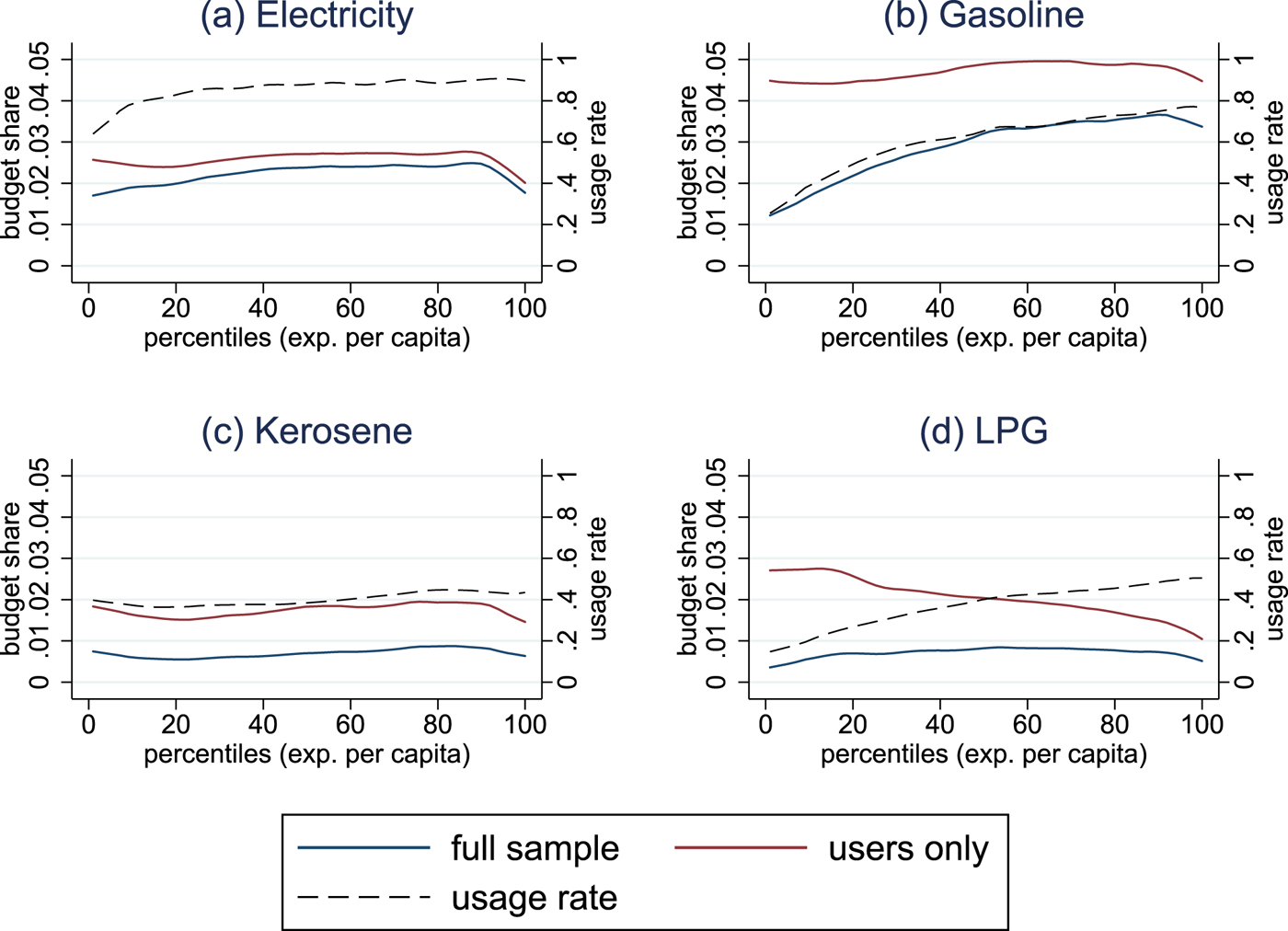
In general, energy expenditures rise over the expenditure distribution, an increase which appears to be driven by transport expenditures. Access to modern domestic energy sources is widespread, though some households below the 20th percentile are without access. Even among this group, more than 90 per cent can access alternatives to solely traditional energy. Figures 1 and 2 set out expenditure patterns for electricity, gasoline, kerosene, and LPG for rural and urban households, respectively.Footnote 6 Due to the discrete nature of the decision to obtain major energy-consuming durables, we distinguish between the average user in the sample, including those with zero demand (demand ≥ 0), and the average user with strictly positive demand (demand > 0). This is a simple approximation of the abovementioned heterogeneity in energy spending patterns between households that, in contrast, may be similar in terms of household per capita income. In the case of the aggregated energy expenditures, this hardly makes a difference, while it is very relevant to the analysis of single energy items. Electricity grid access in Indonesia is high, with 76 per cent of households connected in 2012 (IEA, 2014). In our survey data, electricity use also includes local power supply and diesel generators, and we even observe that 90 per cent of households have non-zero electricity demand. Electricity budget shares, on average, increase with income and are one percentage point higher for urban than for rural households.

Figure 1. Rural energy expenditure shares and usage rates.
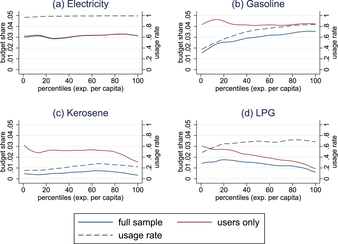
Figure 2. Urban energy expenditure shares and usage rates.
According to figures 1b and 2b, moving from the poorest to the richest households doubles gasoline expenditure shares, for rural and urban households alike. Yet among households that use gasoline, expenditure shares remain stable and, for this subgroup, the first-order distributional effects of a gasoline tax would show a remarkably different pattern. Thirty per cent of the poorest households use gasoline, mostly as an input for motorcycle transport. Kerosene is now the least popular fuel in Indonesia, with only 30 per cent of households exhibiting positive demand. It is still more widely used in rural areas and, somewhat surprisingly, not just by low-income households but also, with slightly higher budget shares, by middle- and higher-income households. While kerosene is a multipurpose fuel, LPG and firewood are mostly used for cooking. In rural areas, LPG shows a very similar expenditure share pattern to kerosene, while usage rates among urban households are substantially higher and expenditure shares are decreasing in wealth. Low-income households depend heavily on firewood and, overall, rural households use more firewood than urban households.
Typically, owning an energy-processing durable is a necessary condition for positive energy demand. Private transport is a case in point for our empirical setting, where the possession of private transport vehicles (specifically motorbikes) explains a large part of gasoline demand. Once households own a motorbike, they tend to spend a similar share of their income on gasoline, irrespective of their income levels. Table 1 illustrates this relationship and depicts poverty status, ownership of a means of private transport, and gasoline expenditure shares across several population subsamples. Out of all urban and rural households, 65.0, 74.0, and 58.2 per cent possess some kind of private transport vehicle, usually a motorbike. Poor households show a 40 per cent lower ownership rate but only slightly lower gasoline expenditure shares than the non-poor. Urban-poor vehicle owners spend an even higher budget share on gasoline than the urban non-poor and, interestingly, we do not find major differences in transport-related energy demand between rural and urban households. Our analysis of energy demand patterns reveals interesting insights on an often-overlooked dimension of the distributional analysis of energy price changes: energy poverty. The International Energy Association defines energy poverty as ‘the lack of access to modern energy services. These services are defined as household access to electricity and clean cooking facilities [e.g., fuels and stoves that do not cause air pollution in houses]’ (IEA, 2014).Footnote 7 Hence, our focus is on the domestically used energy items electricity, kerosene and LPG, for which expenditure information is available in the household survey. We transform quantities of energy items into physical, normalised units (kilograms of oil equivalent, kgoe) and aggregate them to household energy use per capita.
Similarly to conventional poverty measurement, energy poverty measures depend heavily on the underlying poverty line. Thus, in the following, we define two poverty lines. Our first energy poverty line (EPL 1) has a cut-off of 50 kgoe of final annual energy per capita. This poverty line is solely based on modern fuels (electricity, LPG and kerosene) and used for cooking and electricity. This energy poverty line is similar to that in Modi et al. (Reference Modi, Lallement and Saghir2005) but with no distinction in the energy services cooking and lighting. We define our second energy poverty line (EPL 2) according to the expenditure poverty line, inspired by Foster et al. (Reference Foster, Tre and Wodon2000). We do this by transforming demanded quantities of all modern energy items into kgoe and performing a nonparametric kernel-weighted local polynomial regression of the quantity used per energy item on total household expenditures per capita for the reference year 2013. The calculated value at the per capita expenditure poverty line can then be directly interpreted as our energy poverty line, at which we calculate the Foster-Greer-Thorbecke (FGT) energy poverty indices. We refrain from calculating a transport poverty line because of conceptual and empirical issues, such as the difficulty of comparing urban and rural energy needs and the missing public transport data. Table 2 displays the calculated FGT energy indices and the per capita energy poverty line EPL 2, which is considerably lower than EPL 1 at approximately 22 kgoe. Although this poverty line is at a relatively low level, the national energy poverty rate is close to 30 per cent, primarily as a result of the rural energy poverty rate of 43 per cent. To be clear, there are many non-income-poor households which do not use more modern energy than the average household at the poverty line. Based on EPL 1, the national energy poverty rate is above 60 per cent. Since many, and particularly rural, households use firewood for cooking and we have excluded it from the analysis, the magnitude is not particularly surprising.
Table 2. Energy poverty
Note: EPL 2 poverty line: 21.82 kgoe.
3. Methodology
3.1 Demand system
There is an extensive literature on the estimation of demand functions based on economic theory. Since the seminal work of Stone (Reference Stone1954), a significant amount of research has been produced, with Deaton and Muellbauer (Reference Deaton and Muellbauer1980a) Almost Ideal Demand System (AIDS) and the quadratic extension of the AIDS, the QUAIDS by Banks et al. (Reference Banks, Blundell and Lewbel1997) among the more prominent ones. The estimation of QUAIDS has been applied to the energy context by West and Williams III (Reference West and Williams2004), Labandeira et al. (Reference Labandeira, Labeaga and Rodriguez2006), Nikodinoska and Schröder (Reference Nikodinoska and Schröder2016) and Tiezzi and Verde (Reference Tiezzi and Verde2016). To our knowledge, no demand system specification of this form has been applied to the energy context in low- and middle-income countries before.
Rank three quadratic logarithmic budget share systems have an indirect utility function of the following form:
 $$ \ln{V} = \left\{ \left[\displaystyle{{\ln{x} - \ln{a(p)}}\over{b(p)}} \right]^{-1} + \lambda(p) \right\}^{-1}.$$
The price indexes log [a(p)] and b(p) are defined as:
 $$\ln{a(p)} = \alpha_0 + \sum_{i=1}^{n}{\alpha_i \ln{p_i}} + \displaystyle{{1}\over{2}} \sum_{i=1}^{n}{\sum_{j=1}^{n}}{\gamma_{ij} \ln{p_i} \ln{p_j}}.$$
 $$b(p) = \prod_{i=1}^{n}{p_{i}^{\beta_i}}.$$
The term λ(p) in the indirect utility function is a differentiable, homogeneous function of degree zero of prices p and defined as:
 $$ \lambda(p) = \sum_{i=1}^{n}{\lambda_i \ln{p_i}},$$
with  $\sum _i{}\lambda _i=0$. The derived expenditure share system is:
 $$w_i = \alpha_i + \sum_{j=1}^{n}\gamma_{ij} \ln{p_j} + \beta_i \ln{\left[\displaystyle{{x}\over{a(p)}} \right]} + \displaystyle{{\lambda_i}\over{b(p)}} \left\{\ln \left[\displaystyle{{x}\over{a(p)}}\right] \right\}^2,$$
where w i is the share of commodity (group) i of total non-durable expenditures x. To be consistent with utility maximization, the following restrictions need to hold:
Adding-up
 $$\sum_{i=1}^{n}\alpha_i = 1; \;\;\;\; \sum_{i=1}^{n}\gamma_{ij} = 0; \;\;\;\; \sum_{i=1}^{n}\beta_{i} = 0; \;\;\;\; \sum_{i=1}^{n}\lambda_{i} = 0$$
Homogeneity
 $$\sum_{j=1}^{n}\gamma_{ij} = 0$$
Symmetry
 $$\gamma_{ij} = \gamma_{ji}.$$
In household expenditure data, recorded zero expenditures are a common problem. The literature usually identifies this data issue as ‘censored’, although censoring may only be a special case of the underlying data generating process. We stick to this discussion and use ‘censored’ as a synonym for zero observations in budget share data. Shonkwiler and Yen (Reference Shonkwiler and Yen1999) show a way to obtain unbiased elasticity estimates in censored system settings. First, a household specific probit model is estimated with the outcome of 1 if the household consumes good i and 0 otherwise. For each household, the standard normal probability density function (pdf) ϕ and the cumulative distribution function (cdf) Φ are calculated by regressing w i on a set of independent variables z i, containing prices for included goods, household total expenditures, sex and age of the household head, an urban dummy and province fixed effects. Secondly, the pdf and the cdf are integrated into the system of equations as follows:
 $$w_{i}^{\ast} = \Phi w_i + \varphi_i \phi.$$
In contrast to Heckman (Reference Heckman1979), this approach makes use of the full sample in both steps of the estimation process. According to Shonkwiler and Yen (Reference Shonkwiler and Yen1999), the estimation of a censored system requires a procedure that uses the whole sample since each dependent variable may have a different pattern of censoring. Budget elasticities can be derived from the share equation (9):
 $$e_{i}^{\ast} = \displaystyle{{\Phi (\mu_i)}\over{w_i}} + 1,$$
with
 $$ \mu_i = \displaystyle{{\partial w_i}\over{\partial \ln{x}}} = \beta_i + \displaystyle{{2\lambda_i}\over{b(p)}}\left\{\ln \left[\displaystyle{{x}\over{a(p)}}\right]\right\}.$$
The uncompensated price elasticity is given by:
 $$e_{ij}^{u\ast} = \displaystyle{{\Phi (\mu_i)}\over{w_i}} + \phi \tau_{ij} \left(1-\displaystyle{{\varphi_i }\over{w_i}}\right) - \delta_{ij},$$
with
 $$ \mu_{ij} = \displaystyle{{\partial w_i}\over{\partial \ln{p_i}}} = \gamma_{ij} - \mu_i \left(\alpha_j + \sum_{k}^{n}{\gamma_{jk}\ln{p_k}} \right) - \displaystyle{{\lambda_i \beta_j}\over{b(p)}} \left\{\ln \left[ \displaystyle{{x}\over{a(p)}}\right] \right\}^2,$$
and δ ij is the Kronecker delta. Compensated price elasticities are derived by the Slutsky equation:
 $$ e_{ij}^{c\ast}= e_{ij}^{u\ast}+e_i^{\ast} w_j.$$
This two-step methodology has been applied in food demand contexts by Yen et al. (Reference Yen, Kan and Su2002) and Ecker and Qaim (Reference Ecker and Qaim2011) amongst others but not yet for energy demand.
The demand system we use consists of four energy goods, electricity, gasoline, kerosene and LPG, as well as a residual ‘other’ category. This category includes all non-durable consumption goods other than the four energy goods.
3.2 Welfare effects
Since the literature on the welfare impacts of subsidy reforms focuses on first-order effects as in Sterner (Reference Sterner2011), we are interested in the necessity of calculating second-order effects taking into account demand substitution. The first-order effects (FO) only require the observed demand and no additional information on substitution behavior due to price changes (Feldstein, Reference Feldstein1972; Deaton and Muellbauer, Reference Deaton and Muellbauer1980b; Stern, Reference Stern, Newbery and Stern1987):
 $$ {\rm FO} = \sum_{i=1}^{n}{w_{i} \displaystyle{{\Delta p_i}\over{p_i^0}}}.$$
The difference between first-order welfare measures, approximated by the budget share and more exact second-order approximations incorporating household demand responses, are well documented in Banks et al. (Reference Banks, Blundell and Lewbel1996). As they demonstrate, the difference between first- and second-order or exact welfare measures can be quite substantial when price changes are non-marginal. They point to another main difference which is created by the distribution of substitution elasticities, which may change the welfare effects considerably if elasticities differ over the income distribution. To account for heterogeneous preferences, we obtain own- and cross-price elasticities (e ij) on the household level following Banks et al. (Reference Banks, Blundell and Lewbel1997). These are then used in a cost of living experiment with the second order welfare loss approximated by a second-order Taylor series expansion of the cost function (Deaton and Muellbauer, Reference Deaton and Muellbauer1980b):
 $${\rm CV} = \sum_{i=1}^{n}{w_{i} \left(\displaystyle{{\Delta p_i}\over{p_i^0}}\right)} + \displaystyle{{1}\over{2}} \sum_{i=1}^n \sum_{j=1}^n w_i e_{ij} \left(\displaystyle{{\Delta p_i}\over{p_i^0}}\right) \left(\displaystyle{{\Delta p_j}\over{p_j^0}}\right).$$
4. Results
We simulate the welfare and energy poverty impact for two stylised scenarios (20 and 50 per cent price increase) and obtain results for single and multiple simultaneous price changes. Given the currently low international oil prices and past trends, scenarios with even higher price increases of up to 100 per cent and above are indeed possible for the coming years. Yet price changes of this magnitude would require us to forecast completely out of sample. As mentioned above, the survey data offers price information for electricity, gasoline, kerosene, and LPG. Unfortunately, we do not have price information for other transport or firewood expenditures and have to exclude them from further analysis. In addition to these scenarios with energy price increases, we also simulate a scenario that interprets the price change as an ad valorem tax rate and redistributes collected tax revenues via lump-sum cash transfers to households. We assume similarity between consumers' responses to price changes due to market mechanisms and those due to taxes, although there is increasing evidence that calls this assumption into question (Rivers and Schaufele, Reference Rivers and Schaufele2015; Tiezzi and Verde, Reference Tiezzi and Verde2016). Since this difference is most likely to play out in the long run, our analysis still offers valid results in the short run.
4.1 Estimation results
Due to the difficulty of the economic interpretation of model coefficients, we report budget elasticities in table 3 and price elasticities in table 4. Following Banks et al. (Reference Banks, Blundell and Lewbel1997), we calculate elasticities for each household individually and construct a weighted average, with the weights generated as the household's share of total sample expenditure for the relevant good. With rising income, the willingness to spend more on electricity increases, transforming it from a necessity to a luxury good at the 90th percentile. We observe high income responses towards gasoline use, with slightly rising budget elasticities all above one and rising over the expenditure distribution. Gasoline is clearly a luxury good for households of all incomes. Kerosene also exhibits budget elasticities close to 1, particularly for lower-income households. LPG is also estimated to be a necessity for all households, although as in the case of kerosene, the quantitative demand declines with rising income.
Table 3. Budget elasticities

Note: Standard errors in parentheses.
Table 4. Price elasticities

Note: Standard errors in parentheses.
Households with different incomes respond quite similarly to price changes for all energy items, which is why we show only one price elasticity matrix for the first, fifth, and tenth expenditure per capita decile. In general, households react strongly to price changes for all energy items. Most own-price elasticities are close to −1, with the strongest response observed for gasoline. Based on the estimations, we expect to find differences between first- and second-order welfare effects, particularly for electricity and gasoline price changes, when high usage rates overlap with relatively large own-price elasticities. The evaluation of cross-price elasticities reveals that not all modern domestic energy items are complements. Electricity and kerosene are weak substitutes, while electricity and LPG are weak complements, more so for households with higher income. The cross-price elasticities between LPG and kerosene are zero, which clearly shows the unimportant role of energy prices for the politically supported conversion from kerosene to LPG. Substitution between private transport in the form of gasoline demand and domestic energy has no general pattern either. Kerosene and LPG are weak substitutes and complements, respectively, for gasoline, while gasoline and electricity-gasoline cross-price elasticities are close to zero. For other countries, the substitutability of energy items appears to be very context specific, as the findings in the empirical literature demonstrate. Tiezzi and Verde (Reference Tiezzi and Verde2016) find complementarity between electricity and gasoline for the United States, while Nikodinoska and Schröder (Reference Nikodinoska and Schröder2016) find the opposite for Germany. Since this is a critical step in the further analysis, we test for the potential bias of different prices through the geographical location of the household by including province-fixed effects and find no significant difference.Footnote 8
4.2 Welfare and poverty effects
A relatively moderate 20 per cent price increase for all four energy items under consideration and averaging over all households per expenditure percentile is displayed in figure 3. As expected, electricity and gasoline make up the biggest part of the welfare losses, with a progressive pattern in both cases. The relative welfare losses for a uniform 20 per cent electricity price increase are between 0.4 and 0.6 per cent of total expenditures for the poorest and richest households, respectively. For gasoline, these relative welfare losses are larger, particularly for richer households, lying between 0.4 and 0.7 per cent. Smaller welfare effects for kerosene and LPG reflect their relatively low usage rates and budget shares. For the domestically used LPG, a price increase would be slightly regressive, but the magnitude is small due to the low usage rates. This could change, however, if more and more households begin using LPG instead of firewood – in rural areas as well. The difference between the upper-bound first-order effects and the lower-bound second-order effects is relatively small at this magnitude of price effects. First-order estimates of welfare losses in the first scenario are 10 per cent higher on average. These welfare losses become more pronounced in the second scenario of a 50 per cent price increase, where the difference increases to over 20 per cent for electricity and gasoline, again with small observed differences for kerosene and LPG (figure 4). Particularly for gasoline, the second-order effects are slightly less progressive. What is responsible for this effect is not a variation in demand responses with rising expenditures, but rather the increase in the usage rate. A larger fraction of households with actual gasoline demand also implies a larger substitution potential. Low-income households which are close to the poverty line and dependent on the use of modern energy are not as strongly represented in these average effects.
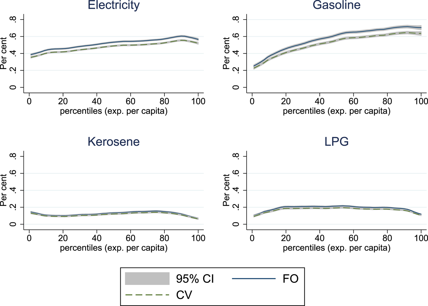
Figure 3. Welfare effects Scenario I.
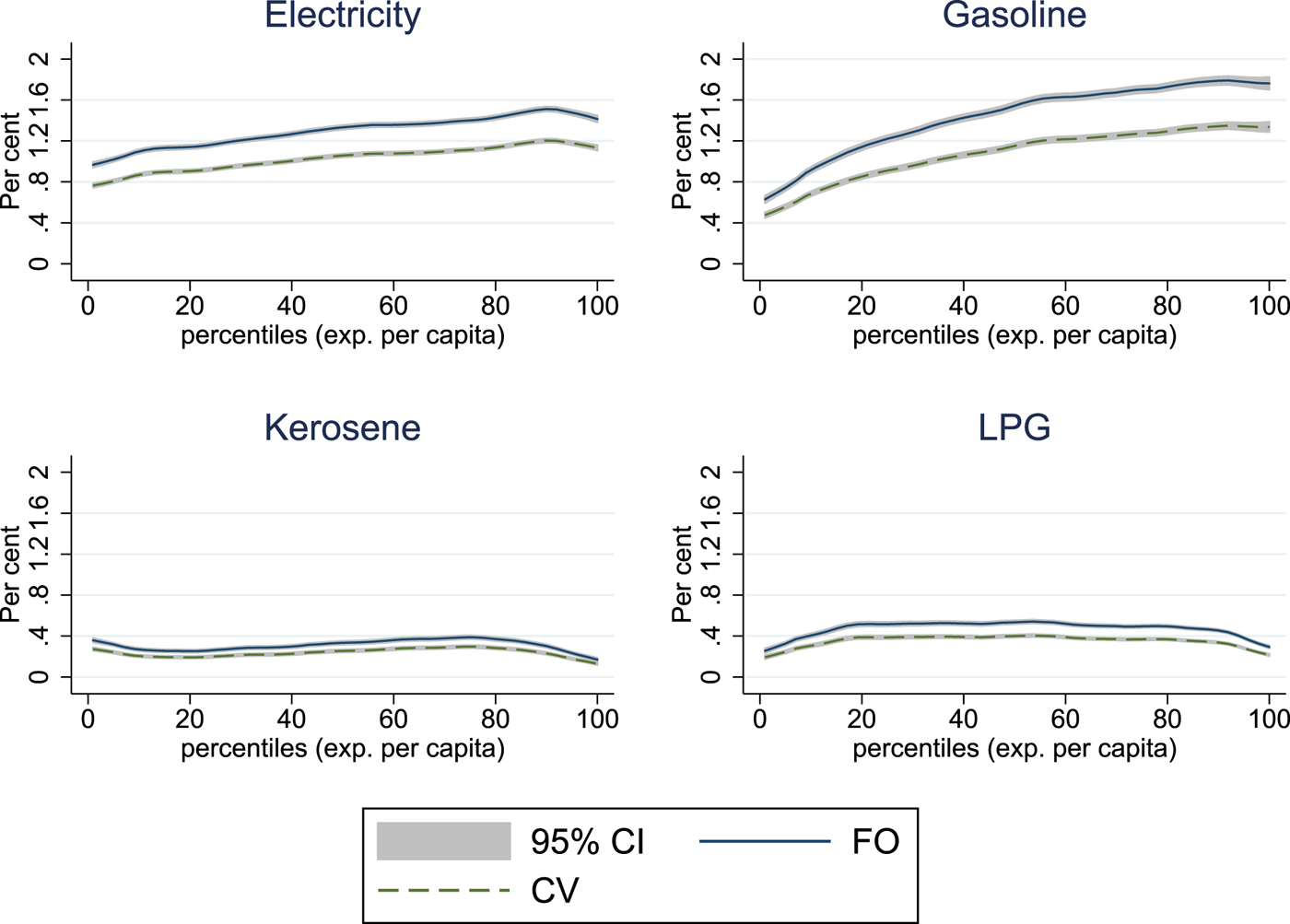
Figure 4. Welfare effects Scenario II.
The poverty indicators in table 5 do not show a large increase, but absolute numbers are important to consider.Footnote 9 The moderate electricity price increases in Scenario I raise the national poverty rate by 0.23 per cent, which appears to be a very small increase but means in absolute terms that approximately an additional half a million people, most of them in rural areas, will be classified as poor. For gasoline price increases, we observe a similar magnitude. Although the poverty effects are relatively small due to the low usage rates and budget shares for modern energy, a significant and growing number of households are negatively affected by price increases. Most of these households are located in urban areas, but with more rural households using modern energy items and private transport vehicles, this finding is unlikely to be stable over time. Non-negligible effects can also be found for LPG price increases, which demonstrates LPG's importance as the new major cooking fuel for Indonesian households.
Table 5. FGT poverty indices (in %), changes from baseline

In the multiple price change scenario, changing prices for all four energy items simultaneously, we observe a general progressive pattern, dominated by electricity and, in particular, gasoline (figure 5). Nevertheless, multiple price changes for the energy items under consideration would result in serious welfare losses for poor households of close to 1.5 and 3 per cent of total expenditures in the case of Scenario I and Scenario II, respectively. Particularly in the case of Scenario II, higher usage rates and associated substitution options for higher income households make the distributional effect less progressive. On the other hand, this lower progressivity also means there is less need to redistribute tax revenue to higher income households, since they are capable of dealing with price increases. The poverty effects are quite strong, with increases of 0.6 and 1.2 percentage points in the poverty rate for Scenario I and Scenario II, respectively.
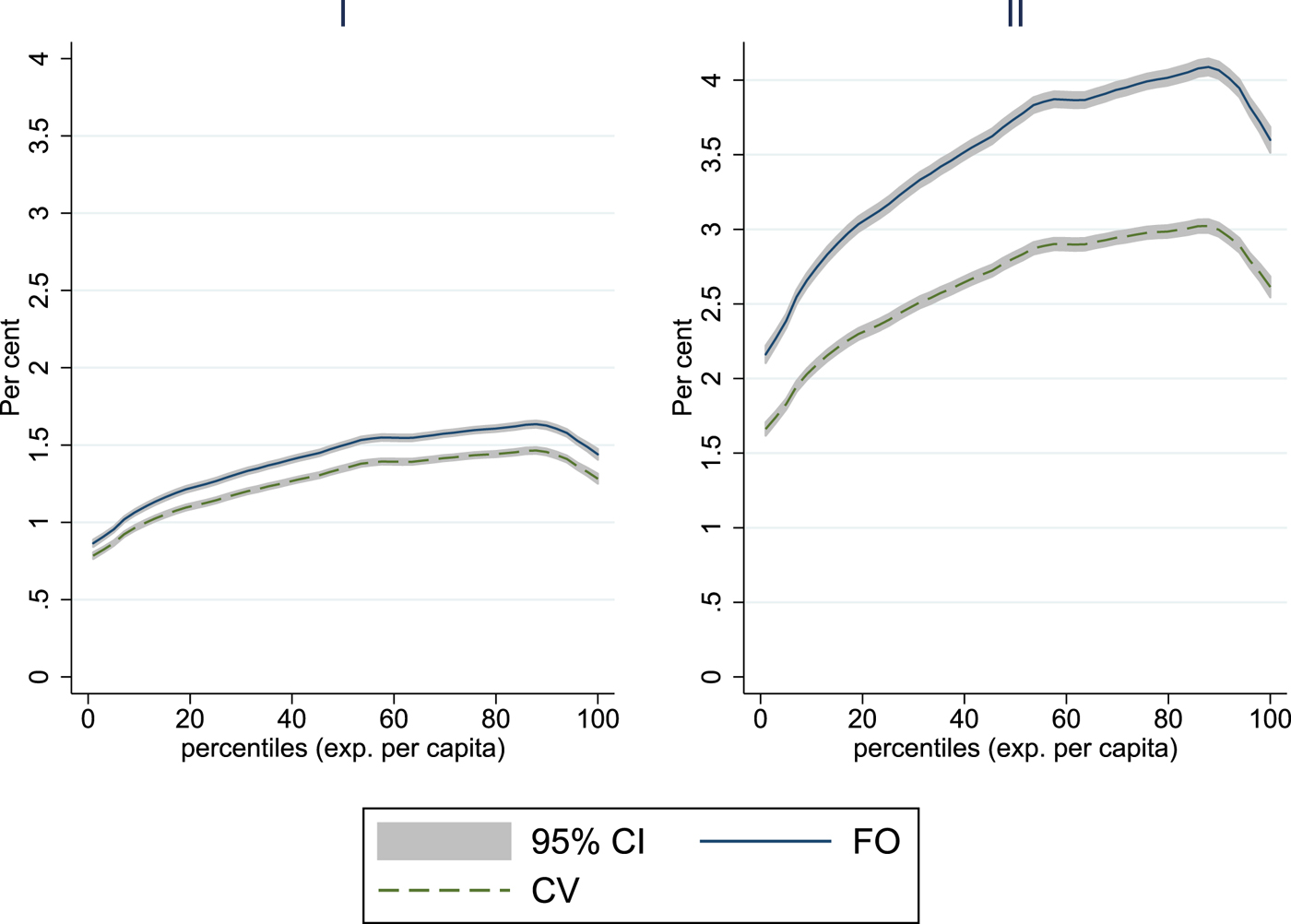
Figure 5. Welfare effects simultaneous increase Scenarios I & II.
To shed some light on the potential effects of redistribution if energy taxes of 20 per cent are the drivers behind the price increases, we simulate a full redistribution of tax revenues via lump-sum transfers to households. For all four energy items, the redistribution of tax revenue leads to welfare gains for low-income households (figure 6). Electricity and gasoline taxes raise substantial revenue, which could lead to quite large welfare gains for the majority of the population if proper redistribution schemes can be identified. Welfare gains are also reflected in the poverty indicators, which improve for all scenarios (table 5). As much as urban households are disproportionately hit by energy price hikes, there are also more urban households which benefit from transfer payments. Since universal lump-sum transfers are unlikely to be implemented, more realistic redistribution schemes would rely on social welfare programmes, which directly target the poor.Footnote 10
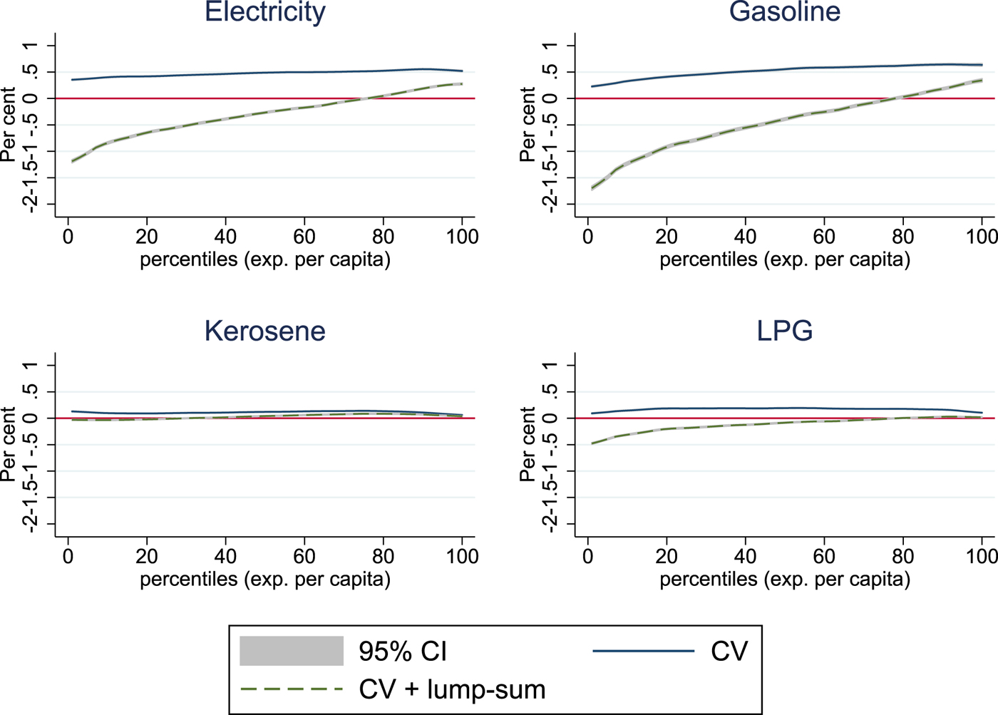
Figure 6. Welfare effects with lump-sum transfers Scenario I.
4.3 Energy poverty
Based on the estimated price elasticity matrices, we calculate the quantities households reduce per capita in response to price increases for the respective scenarios. Based on these behavioural responses, we calculate the FGT class of indices for both scenarios and energy poverty lines and find significant effects on energy poverty resulting from lower energy use. Table 6 displays the change in FGT indicators for the two simulated scenarios. We find that price increases have considerable effects on the poverty rate, with particularly tremendous effects in the case of electricity and LPG price increases. LPG price increases result in higher energy poverty levels than kerosene price increases, with the latter demonstrating the smallest effects, as expected. For all modern fuels, the increase in energy poverty is greater in rural areas, despite the higher urban usage rates. As discussed in the interpretation of estimated price elasticities, complementarity between LPG and gasoline implies reduced domestic energy use, also in the case of gasoline price increases. Energy poverty increases due to gasoline price changes are approximately 25 per cent of those resulting from LPG price increases, a value close to the estimated cross-price elasticity. The redistribution of tax revenues does not significantly change energy poverty since households are projected to spend most of the extra income on goods other than energy.Footnote 11
Table 6. FGT energy poverty indices (in %), changes from baseline

These findings reflect the downside of consumer responses and the associated smaller welfare effects through substitution. While the microeconomic welfare metric tells us only about utility-based monetary effects, other welfare dimensions such as energy poverty are not directly addressed in a standard welfare assessment. Although one could argue that households take energy requirements into account in consumption decisions, they are also likely to substitute traditional fuels for modern fuels when prices rise. Additionally, they may not internalise all associated external costs such as health issues caused by air pollution. Unfortunately, our data does not permit us to quantify the exact nature of substitution between modern and traditional fuels when prices change. However, a simple estimation of firewood demand in a Working-Leser form (Working, Reference Working1943; Leser, Reference Leser1963) depending on prices for modern energy sources, household total expenditures x, and household characteristics H sheds some light on this issue:
 $$ w_{\rm fwd} = \alpha_{\rm fwd}+ \sum_{j=1}^{n}\gamma_{ij} \ln{p_j} + \ln(x) + H. $$
Due to a significant share of zero firewood budget shares, equation (17) is estimated as a Heckman selection model with additional variables reflecting lighting and cooking fuel choice in the identifying equation.Footnote 12 The estimated firewood cross-price elasticities (table 7) exhibit an expected substitutability between the other domestically used energy items – electricity, kerosene, and LPG – and firewood. This provides some evidence, though it is not integrated into the rest of the analysis due to data constraints, that households are very likely to increase the use of traditional fuels when prices of modern, domestically used energy items rise. Households may not reduce domestically used energy as strongly as energy poverty indices suggest, but instead move towards traditional fuels.
Table 7. Firewood cross-price elasticities

Such behaviour is in line with the literature on the energy ladder that provides evidence on the effects of modern energy prices on traditional fuel use (Leach, Reference Leach1992; Heltberg, Reference Heltberg2005; Gebreegziabher et al., Reference Gebreegziabher, Mekonnen, Kassie and Köhlin2012). Unlike the discrete choice models in this literature, the estimated Working-Leser model represents a structural approach that allows for insights on how much the quantity of traditional fuels used changes in response to a price change of modern fuels.
5. Conclusion
Consumer energy price increases affect richer households more in relative terms, and therefore also in absolute terms. On the one hand, our findings confirm prior studies, which are based on observed demand and the assumption of zero substitution between goods, on the progressive direction of this effect for electricity and gasoline. On the other hand, we find neutral effects for kerosene and LPG and smaller welfare losses for electricity and gasoline by employing second-order welfare estimates. The calculated first-order effects for electricity and gasoline are on average 10 and 20 per cent larger in Scenario I and Scenario II, which may seem small in relative terms but represent substantial differences in absolute terms. First-order effects particularly overestimate welfare losses for the upper part of the income distribution, where small percentage changes in relative terms translate into large absolute monetary amounts. This has important consequences for redistribution, since richer households are estimated to be capable of dealing with increasing energy prices and therefore less in need of compensation. This holds particularly for gasoline, which is at the centre of the subsidy debate and a major fuel used by households. Due to low-income households' lower usage rates, the poverty impacts are also moderate when prices change by small amounts.
Despite these supposedly small relative changes, a non-marginal number of low-income households are highly affected by energy price changes. Additionally, a substantial and growing number of households are vulnerable to large energy price increases, which may be quite likely when energy subsidies are completely abolished. Ultimately, the redistribution of taxes or saved subsidies is crucial to turning this story around to create welfare gains and poverty reduction. Although the simulated lump-sum transfers are quite effective in absorbing large welfare shocks, more targeted transfers are certainly desirable from an equity and fiscal perspective. The estimation of a demand system proves to be useful for calculating welfare effects, and the consideration of energy poverty and household-related carbon emissions makes it even more valuable. Without changes in the quantities demanded being taking into account, the degree of energy poverty would not change in our expenditure based definition of energy poverty. In addition to welfare losses from energy price increases, households also suffer from a lack of modern energy items, which could trigger additional negative impacts such as adverse health effects through the shift to traditional sources of energy. By simulating energy item quantities, we find that price increases for energy used domestically have substantial effects on energy poverty. Somewhat surprisingly, this also holds for gasoline, since the estimation reveals a complementary relationship to LPG. This complementarity is particularly problematic for low-income households, for which these energy goods have much more of a necessity character than they do in high-income households. The resulting divergence of relatively small estimated second-order welfare effects and large impacts on energy poverty reflects a weakness of standard welfare metrics, which assumes complete information and the absence of negative externalities.
Additionally, the redistribution of tax revenue is only partially able to deal with rising energy poverty in our model since households spend most of the transfer income on goods other than modern energy. The resulting increased use of traditional biomass fuels such as firewood is certainly critical from both a health perspective, due to indoor air pollution, and a CO2 emissions perspective, due to deforestation.Footnote 13
For all simulated effects, we have to keep in mind that households can only reduce energy use to a certain minimum level. This and the nature of our modeling framework restricts the interpretation of results to the very short-run perspective.


 Open access