


1. Introduction
The impact of a structure on a wavy or quiescent water surface is a complex phenomenon in which many physical processes are involved. Typically, the impact generates highly transient impact loads, rapid structural deformation and violent water surface motion, including the formation of waves and high-speed sprays. These physical processes interact with each other over short time scales and the rates of change of many physical quantities are substantial. In addition, under certain circumstances, air can be entrained into the flow system and the resulting two-phase flow may affect the flow dynamics and acoustics. In an effort to study the physics of impact phenomena, investigators have taken advantage of simplified structure geometries and motions typically during impact with calm water surfaces. A number of these studies are discussed briefly below.
The classic problem of the vertical water entry of a rigid wedge at high Froude number has been studied extensively in a two-dimensional potential flow framework; see, for example, Wagner (Reference Wagner1932), Dobrovol'Skaya (Reference Dobrovol'Skaya1969) and Zhao & Faltinsen (Reference Zhao and Faltinsen1993). These models explain the dynamics of this flow in which the water surface overturns as it rises along the tilted surface of the wedge. The region where the flow overturns is called the spray root. The theory is based on the assumption of a self-similar flow with constant wedge velocity and predicts a high pressure ridge that moves along the wedge surface with the spray root. Extended mathematical models for the water entry of rigid objects of various geometry were developed in studies such as Howison, Ockendon & Wilson (Reference Howison, Ockendon and Wilson1991), Vorus (Reference Vorus1996), Xu et al. (Reference Xu, Troesch and Vorus1998), de Divitiis & de Socio (Reference de Divitiis and de Socio2002), Moore et al. (Reference Moore, Howison, Ockendon and Oliver2012) and Wu & Sun (Reference Wu and Sun2014).
The physics of the impact of rigid objects on a water surface has also been studied through experiments. Early experimental studies on the gravity-driven free drop of a rigid wedge or three-dimensional objects on a water surface were reported by Chuang (Reference Chuang1966), Chuang & Milne (Reference Chuang and Milne1971) and Chuang (Reference Chuang1973). These studies largely confirm the theoretical findings discussed above. Experiments performed by Judge, Troesch & Perlin (Reference Judge, Troesch and Perlin2004) on the vertical/oblique impact of a tilted wedge on a water surface illustrated the effects of the wedge's initial velocity ratio and the level of asymmetry from the vertical axis at its vertex on the symmetry of the spray root propagation as well as on the flow separation from the wedge's surface. Mathematical models for the water entry of an asymmetric wedge are developed in studies such as Semenov & Iafrati (Reference Semenov and Iafrati2006) and Semenov & Wu (Reference Semenov and Wu2018). Breton, Tassin & Jacques (Reference Breton, Tassin and Jacques2020) performed an experimental study on the vertical water entry/exit of axisymmetric bodies. The evolution of the wetted surface under the body and the force on the body during the process were measured. The effect of gravity on the impact at low initial impact velocity is pointed out by the authors. Experimental investigations on the vertical impact of an inclined nearly rigid plate with prescribed impact velocity on a water surface were performed by Wang et al. (Reference Wang, Wang, Balaras, Conroy, O'Shea and Duncan2016) and Wang & Duncan (Reference Wang and Duncan2019). In Wang & Duncan (Reference Wang and Duncan2019) the effect of gravity on the evolution of the spray over time was characterized by an instantaneous Froude number associated with the temporally varying nominal submerged length of the plate. Iafrati (Reference Iafrati2016) performed an experimental study on the ditching of a rectangular plate of negligible deformation into the water surface with substantial horizontal velocities just before the impact. The study shows that the propagation speed of the pressure peak on the plate relative to the geometrical intersection of the plate with the still water surface varies over time and the impact load scales favourably with the velocity normal to the plate. It is also worth noting that if the local inclination of the impactor is small near the touchdown point, due to the flow induced by the air cushion between the impactor and the water surface, the water surface can deform before the impact. The effect of the air cushion is especially important for phenomena at the very initial stage, when the instantaneous Froude number is tremendously large. The detailed behaviour of the air cushion and its effect on various aspects of the impact, such as splash, pressure and force, are studied in, for example, Bouwhuis et al. (Reference Bouwhuis, Hendrix, van der Meer and Snoeijer2015), Jain et al. (Reference Jain, Gauthier, Lohse and van der Meer2021), Moore (Reference Moore2021), Hicks et al. (Reference Hicks, Ermanyuk, Gavrilov and Purvis2012).
The impact of a vertically moving flexible wedge on a water surface was also investigated extensively in the past (see, for example, Maki et al. Reference Maki, Lee, Troesch and Vlahopoulos2011; Luo, Wang & Soares Reference Luo, Wang and Soares2012; Khabakhpasheva & Korobkin Reference Khabakhpasheva and Korobkin2013; Panciroli, Abrate & Minak Reference Panciroli, Abrate and Minak2013; Piro & Maki Reference Piro and Maki2013; Shams & Porfiri Reference Shams and Porfiri2015; Shams, Zhao & Porfiri Reference Shams, Zhao and Porfiri2017; Yu, Li & Ong Reference Yu, Li and Ong2019; Zhang et al. Reference Zhang, Feng, Zhang, Chen, Sun and Zong2021). Panciroli (Reference Panciroli2013) indicated that the deformation of a flexible wedge can cause the separation of the spray sheet from the wedge surface. The results shown in Shams et al. (Reference Shams, Zhao and Porfiri2017) by model and experiments on the free falling of a rigid/flexible wedge on a water surface indicate a very limited effect of hydroelasticity on the spray root propagation during the water entry stage. However, the results indicate that the impact force is reduced as the structural deformation increases during the water entry stage of the gravity-driven wedge. The reduction of the impact force during the gravity-driven vertical impact of a wedge with flexible panels is also illustrated by Ren et al. (Reference Ren, Wang, Stern, Judge and Ikeda-Gilbert2019) and Ren, Javaherian & Gilbert (Reference Ren, Javaherian and Gilbert2021). It should be pointed out that in a gravity-driven impact, the variation of the hydrodynamic force induced by deformation also modifies the rigid body motion of the impactor and in turn changes the flow characteristics and impact force. Therefore, it is difficult to decouple the effect of the deformation on the impact force.
During the vertical water entry of a flexible wedge, an important parameter that characterizes the effect of hydroelasticity is the ratio between the characteristic impact time (wetting time) to the natural period of the panel (Faltinsen Reference Faltinsen1999; Panciroli et al. Reference Panciroli, Abrate and Minak2013). For a gravity-driven vertical impact of a flexible wedge on a water surface, the wetting time is also associated with the mass of the wedge, in addition to the initial impact speed, the deadrise angle and the distance between the vertex and the chine.
Faltinsen & Semenov (Reference Faltinsen and Semenov2008) performed a theoretical study on the oblique water entry of a rigid two-dimensional (2-D) plate. The oblique impact calculations presented in the work of Faltinsen & Semenov (Reference Faltinsen and Semenov2008) cover a range with relatively small horizontal-to-vertical entry velocity ratios (smaller than 2.75) as well as a relatively large pitch angle (greater than 15 $^\circ$). The variation of the pressure and normal force coefficients are shown under various combinations of the velocity ratio and the plate pitch angle. Reinhard, Korobkin & Cooker (Reference Reinhard, Korobkin and Cooker2013) performed a theoretical study on the oblique impact of an elastic 2-D plate with free ends on a water surface at large horizontal speed. The calculation indicates that the elastic deformation of the plate may increase the impact force and the chance of cavitation, both due to the low fluid pressure induced by the plate vibration. It should be noted that the calculation is performed with a free-end boundary condition and rigid body motion of the plate is not prescribed.
In the experimental investigation on the impact of a fuselage specimen on a water surface by Iafrati & Grizzi (Reference Iafrati and Grizzi2019), cavitation and ventilation, triggered by the curved shape of the specimen, were observed when the horizontal velocity is sufficiently large. It is pointed out that the cavitation and ventilation have a significant influence on the impact load. In a computational study on the 2-D oblique impact of an elastic plate (beam) with free-free boundary condition at both ends on a thin liquid layer, Khabakhpasheva & Korobkin (Reference Khabakhpasheva and Korobkin2020) also show the possibility of air entrainment as a consequence of plate deformation and rotational motion. Spinosa & Iafrati (Reference Spinosa and Iafrati2021) conducted an experimental study of the water impact of aluminum plates at large horizontal speed and it is pointed out that the structural deformation causes a reduction in peak pressure and an increase in the total load. Faltinsen (Reference Faltinsen1999) proposed an orthotropic plate theory for the coupled analysis of the structural dynamics and the flow motion during the vertical water entry of a ship panel. It is pointed out that the hydroelastic response increases as the ratio of the wetting time to the lowest order natural period of the panel decreases. Wang et al. (Reference Wang, Kim, Wong, Yu, Kiger and Duncan2019) performed an experimental study on the oblique impact of a flexible and a rigid plate with non-zero pitch and roll angles. Under the same motion trajectory, it is found that the maximum deformation of the flexible plate occurs at a more downstream location for a greater impact speed. It is also found that the outboard spray generation during the impact is influenced by the plate deformation.
The impact of a horizontally oriented elastic flat plate falling on a wave crest is studied theoretically by Kvålsvold & Faltinsen (Reference Kvålsvold and Faltinsen1995), Faltinsen (Reference Faltinsen1997), Faltinsen, Kvålsvold & Aarsnes (Reference Faltinsen, Kvålsvold and Aarsnes1997) and Korobkin & Khabakhpasheva (Reference Korobkin and Khabakhpasheva2006). Faltinsen (Reference Faltinsen1997) suggested that the impact process can be categorized into an initial structural inertial phase, which is a very short period during which the plate does not have enough time to rebound before the plate is completely wet, and a subsequent free vibration phase of the plate with associated added mass. It is also shown experimentally by Faltinsen (Reference Faltinsen1997) and Faltinsen et al. (Reference Faltinsen, Kvålsvold and Aarsnes1997) that the maximum bending stress in the plate is not sensitive to the relative location of the wave crest on the plate nor the radius of curvature of the wave crest in the impact region. It is pointed out by both Faltinsen (Reference Faltinsen1997) and Korobkin & Khabakhpasheva (Reference Korobkin and Khabakhpasheva2006) that cavitation and/or ventilation can occur during the impact, as a result of the plate deformation.
In the present study the oblique and vertical impact of flexible plates on a quiescent water surface is investigated experimentally. This study includes several features that have not been examined in the above-mentioned experimental studies. First, the plate is driven into the water surface while its velocity is held constant during the time interval between the passage of the plate's trailing (lower) and leading (upper) edges through the still water level (SWL). (The plate is pitched at a 10 $^\circ$ angle.) Second, the force and moment required to maintain the steady plate motion are measured during the impact. And finally, the plate flexibility is varied from stiff, creating maximum deflections of only a few millimetres even at the highest impact speeds, to the very flexible, creating large maximum deflections, on the order of 50 mm. These large deflections create two-way fluid–structure interactions in which the hydrodynamic force and moment change compared with those found during a rigid plate impact at the same velocity. Also, the set-up and wide range of highly controlled experimental conditions allow for a parametric investigation of the interaction between the structural response and the fluid motion.
Some of the data from the present study were used in Wu & Earls (Reference Wu and Earls2021) and Pellegrini et al. (Reference Pellegrini, Diez, Wang, Stern, Wang, Wong, Yu, Kiger and Duncan2020) for validation of fluid–structure interaction numerical codes.
In the remainder of this paper, the details of the experimental set-up, measurement techniques and experimental conditions are described first in § 2. In § 3 the experimental results are presented along with analysis and discussions. Finally, the concluding remarks are given in § 4.
2. Experimental details
In this section the details of the experimental set-up, procedures and conditions are described in detail. This description is divided into a series of subsections with the experimental facilities, the force and moment measurements, the flexible plates, the plate deflection measurements, the under-plate spray root measurements, the measurements of the plates’ free vibration frequencies and the experimental conditions and procedures given in § 2.1 to § 2.7, respectively.
2.1. Experimental facilities: towing tank and two-axis carriage
The experiments were performed in the towing tank facility in the hydrodynamics laboratory at the University of Maryland. A schematic of the facility is given in figure 1. The tank is 13.41 m long, 2.45 m wide and 1.33 m tall and consists of a series of 35 mm-thick transparent acrylic side and bottom panels that are bolted to a steel superstructure frame. The frame is in turn bolted to the concrete floor of the laboratory. Another steel superstructure frame (herein called the carriage support frame) is positioned next to one of the long sidewalls of the tank and spans its entire length. The frame is 3.7 m tall and is bolted to the laboratory's concrete floor and sidewall. Two precision horizontal rails, which span the length of the tank, are bolted to two very stiff steel box beams which are in turn bolted to the carriage support frame. A two-axis towing carriage, designed and built for the present experiments, runs along the two horizontal rails. The horizontal motion of the carriage is driven by a belt that is in turn driven by two hydraulic servo motors that are attached to the carriage support frame and powered by a 44 kw hydraulic power unit. The carriage support frame is not in contact with the towing tank, thus avoiding any undesired tank vibration or water surface motion induced by the motion of the carriage.

Figure 1. Schematic drawing of the towing tank and high-speed carriage system. The interior side and bottom panels of the tank are made of clear acrylic to allow for flow visualization. The flexible plates are attached to the two-axis carriage that is driven horizontally along one side of the towing tank by a belt and hydraulic servo motor system. The vertical carriage rides on rails that are attached to the horizontal carriage and is driven by a belt and electric servo motor system. Camera 1 is installed under the tank for the measurement of the under-plate water surface motion. Cameras 2–4 are installed along the tank's side wall for the measurement of the plate deflection.
The two-axis towing carriage, as shown in figure 2(a), is made of 304 stainless steel and consists of a horizontal carriage, which moves along the two horizontal rails described above, and a vertical carriage, which moves along two vertical precision rails that are bolted to the horizontal carriage. The horizontal and vertical carriages are constructed from stiff frames, composed from a series of I-beams and bulkhead stiffeners, with a sheet metal skin (12 and 14 gauge thickness) riveted to the frames. The horizontal carriage carries an electric servo motor and a belt-sprocket motion system that drives the vertical carriage. The instantaneous positions of the horizontal and vertical carriages are measured with an absolute rotary encoder (model 1037504, SICK Sensor Intelligence) and a linear position sensor (Temposonics R-series model RH, MTS, Inc.), respectively, at a sample rate of 1024 Hz. Motions of both axes are controlled by a position feedback control system through a computer.

Figure 2. Schematics drawings of the carriage and flexible plate. In (a) the structure of the two-axis high-speed carriage and the dynamometer system are shown. The coordinate system of the undeformed plate is denoted. The origin of the coordinate system is at the undeformed plate's centre,  $O$, and the longitudinal, transverse and normal coordinates are denoted as $\hat l$, $\hat t$ and $\hat n$, respectively. In (b) a side view of the dynamometer system and some details of the plate mounting mechanism are shown. The direction of the horizontal and vertical carriage velocities, $U$ and $W$, and the orientation of the water surface, are denoted. The pitch angle of the plate is denoted as $\alpha$. The five locations where the out-of-plane deflection is measured are denoted as $R_i$ ( $i=1,\ldots,5$). The locations of $R_i$ are at the transverse mid plane ( $t=0$) and are equally spaced between the axes of the two shafts, with $R_3$ at the plate centre. In (c) the projected view of the dynamometer system and the plate is shown when viewed toward the positive longitudinal direction. The numerical values of the dimensions labelled in the figure are as following: $\alpha =10^\circ$, $L=1080$ mm, $L_s=1016$ mm, $l_1=L_s/6=169.3$ mm, $d_1=38.1$ mm, $d_2=28.6$ mm, $B=406$ mm and $B_s=269$ mm. In (d) a detailed schematic of a single deflection sensor is shown.
2.2. Plate mounting structure and force/moment measurement system
The impact plate is installed under the vertical carriage through a mounting structure that includes four struts, a dynamometer and two rotary bearing systems, as shown in figure 2. The struts are right angle beams made of aluminum alloy. In the present experiments the lengths of the four struts are chosen to create a 10 $^\circ$ pitch angle and 0 $^\circ$ roll angle for the plate. The dynamometer includes two parallel frames made of square box beams and stiffeners. The upper and lower dynamometer frames are connected at each of the four frame corners through a dynamic three-component load cell with thick steel mounting blocks (Kistler 9367C, 60 kN range, with 5080A multichannel charge amplifier); see figure 2(a). With this configuration, the dynamometer can measure all three components ( $l$-longitudinal, $t$-transverse and $n$-normal; see figure 2a) of the total force and the total moment, exerted by the lower frame and its attachments to the upper frame.
The impact plate is connected to the lower frame of the dynamometer using a linear bearing system (SRB2-08SS-016, PBC Linear) at the forward and aft ends of the dynamometer frame; see figure 2. In this configuration, one bearing is centred on and bolted to the bottom of each load cell unit. Near each of the transverse plate edges, herein called the leading edge or the trailing edge (labelled in figure 2b), an aluminum T-rail that is bolted to a stainless steel round shaft (diameter 12.7 mm) is bolted to the plate. The relatively thick T-rail covers the entire plate width and is bolted to the plate with pairs of machine screws placed every 50.8 mm across the plate width. The flat heads of the screws are counter sunk into the bottom surface of the plate so as to minimize their effect on the water flow during the experiments. With this configuration, the plate bending along the two transverse edges is believed to be small under a nearly uniformly distributed load along the transverse direction, as in the present experiments. Each round shaft goes through two rotary bearings described above and is free to rotate about the axis of the shaft. The translation of each shaft along its axis is prevented by shaft collars. With this configuration, the shaft, which is centred 28.6 mm ( $d_2$, see figure 2) above the upper surface of the plate and at a longitudinal distance of 32 mm away from the plate's leading/trailing edge, is only allowed to rotate about its axis while rotation about other directions and translation along any directions are prohibited. This mounting configuration is analogous in some way to a plate simply supported at two opposite edges and free at the other two opposite edges. However, one should keep in mind that the rotational axis of the present configuration is above the plate and inward of the plate's leading and trailing edges.
The impact plates used in the present experiments are all made of aluminum 6061-T651 alloy (density of  $\rho _p=2700\,{\rm kg}\,{\rm m}^{-3}$; elastic modulus of $E=68.9$ GPa; Poisson's ratio $\nu _p=0.3$). Three impact plates are used in the present experiments. All plates are $L=1080$ mm long by $B=406$ mm wide while their thicknesses varied from plate to plate. Next to the port edge of the plate, a very stiff vertical wall that reaches the tank bottom is installed along the tank. The distance between the vertical wall and the plate's port edge is 2 mm and remains nearly constant along the length of the wall.
The impact force and moment are sampled using an A/D system (PXIe-4497, National Instrument) with a sample rate of 40.96 kHz. Double shielded cables are used to avoid the electrical noise contamination from the vertical carriage servo motor system. The manufacturer's calibration data of each load cell was verified and the total force/moment measured by the dynamometer was also verified by applying standard weights to the individual load cells and to the dynamometer frame at various locations, respectively.
2.3. Thickness of the impact plates
In order to evaluate the uniformity of the plates and to obtain a statistical description of each plate's thickness, an ultrasonic thickness meter (GE CL5 Krautkramer, with Alpha2-DFR probe) was used to measure the plate thickness at both the edges and the interior of the plate. Before measuring the thickness of each plate, the ultrasonic meter was calibrated by the thickness at the edge of the same plate which was also measured with a high-precision micrometre in a small section where the paint on the lower surface was removed. The ultrasonic probe was then placed at a series of  $22 \times 8$ grid points with 50.8 mm spacing on the upper side of the plates for the measurements, so that only the aluminum thickness was captured by the ultrasonic meter; in this configuration the thickness of the very thin layer of paint on the lower side of the plates does not affect the measurements. The measurement resolution of the ultrasonic meter is 0.001 mm. The statistics of the thicknesses at a total of 176 measured locations for each plate are listed in table 1. The results indicate that the thickness of each impact plate is highly uniform with a range of variation of approximately 0.1 mm and a standard deviation of approximately 0.02 mm. In the following discussion, the mean thicknesses of the three plates will be used in the data analysis.
Table 1. Statistics of the thicknesses of the three impact plates, measured by an ultrasonic thickness meter at 176 grid points on each plate.

2.4. Plate deformation measurement
The out-of-plane deflection of the plates is measured at five locations along the longitudinal plate centreline. All five measurement locations lie between the axes of the two plate mounting shafts and are equally spaced by a distance of 169.3 mm ( $l_1$, see figure 2). The out-of-plane deflection gauge employed in this study consists of a metal rod whose lower end connects to a swivel joint that is glued to the plate's upper surface; see figure 2. The rod goes through a hole on a ball joint fixed on a frame that is in turn bolted to the four dynamometer mounting struts. An imaging target, a white board with a random black dot pattern printed on it, is installed at the tip of each metal rod and at the fixed ball joint. As the plate deforms, the relative distance from the target at the rod tip to the target on the fixed ball joint varies. Three high-speed cameras (cameras 2–4 in figure 1, model V640, V641, VEO 640L, Vision Research Inc.) are installed along the side of the tank to record the motion of these imaging targets at a frame rate of 1024 Hz and a field of view of 98 cm by 61 cm. Flood lights were installed along the side of the tank to provide illumination for the imaging. The camera image sensors measure 2560 by 1600 pixels resulting in a 0.38 mm pixel $^{-1}$ resolution. Each black dot on the imaging target is 2.25 mm (5.9 pixel) in diameter and there are 25 dots in each image of the target. The processing aims at finding the relative displacement vector of the same target between the first image of the target in each camera and the current image of the target by using cross-correlation values of the image intensity map between the two images. A three-point Gaussian peak fit to the three highest cross-correlation values around the peak was used to achieve sub-pixel accuracy of the displacement. Calibration experiments were performed in which one of the dot-pattern targets was attached to a linear translation stage with an accuracy of 0.0127 mm and photographed at 100 successive locations separated by 0.0254 mm (total displacement $= 2.54$ mm). Using various combinations of pairs of images, correlations were performed for at least 50 pairs of images for relative target displacements ( $\varDelta$) ranging from 0.0254 mm to 1.27 mm. It was found that a displacement of 0.1 mm was measured by this system with a standard deviation of $\pm$7 %.
2.5. Under-plate water surface measurement
The water surface evolution under the flexible plates was also recorded during the impact experiments. For this purpose, a high-speed camera (camera 1 in figure 1, model V640, Vision Research Inc. 2500 by 1600 pixel sensor), a flat mirror oriented at a 45 $^\circ$ angle from the horizontal plane, and two flood lights were installed under the towing tank near the impact site, as illustrated in figure 1. With this configuration, the camera views the plate's lower surface and the under-plate water surface, through the transparent tank bottom panel. Flat white paint was sprayed uniformly over the lower surface of each flexible plate in order to provide a uniformly illuminated background for observing the water surface evolution. Grid lines were then added to each painted surface with spacing of 50.8 mm to inform the location of water surface features relative to the plate surface.
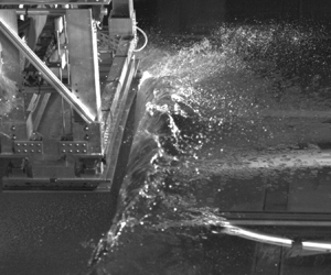
A sample image taken from one of the high-speed movies during an impact of the thinnest plate is given figure 3. The location of the spray root, defined in the following, is extracted from each image. During impact, the water surface rises between the plate's geometrical intersection with the SWL and the plate's leading edge, and, via a region called the spray root, overturns to join a thin spray sheet which extends over time along the plate's lower surface as the impact proceeds (see, for example, studies of the vertical impact of a wedge/plate on a water surface, Zhao & Faltinsen Reference Zhao and Faltinsen1993; Wang & Duncan Reference Wang and Duncan2019). The under-plate spray root line is a spatial curve consisting of points on the under-plate water surface where the surface normal becomes horizontal. In the region between the spray root line and the plate's trailing edge, the left side of the image in figure 3, the camera views the lower side of the plate only through the water phase. Thus, this region appears smooth in the images. In the region between the spray root line and the plate's leading edge, to the right in figure 3, the image of the plate appears rough, due to the rough surface of the under-plate spray sheet (caused by the growing turbulent boundary layer within the spray sheet and gravitational instability) and the rough lower water surface (caused by splashes due to falling droplets and ligaments). In the images, the spray root line separating these two regions appears as a narrow opaque band, due to the total internal reflection of the subsurface light rays that reach the spray root region. The edge of the band closest to the plate trailing edge is taken as the location of the spray root line, and is marked in figure 3. Using measurements of the actual distance of the spray root from the surface of a wedge during vertical impact, Wang & Duncan (Reference Wang and Duncan2019), and the camera viewing angle relative to the normal to the plate surface in the present experiments (4 $^\circ$ to 24 $^\circ$), it is estimated that the error between the true position of the spray root and that measured by the above method is at most $0.004L$.

Figure 3. An image from a high-speed movie taken looking up from under the tank during an impact of the thinnest plate for  ${Fr} = 0.43$ and $UW^{-1}=8.33$. The spray root line is visible as marked in the image. The camera and flood lights set-up is shown in figure 1. The plate is moving from left to right and the image was taken at $t/T_s = 0.50$.
The coordinates of the spray root line in the reference frame of the plate's lower surface at a set of equally spaced times during impact are obtained by the following method. The times when the spray root line crosses each grid point are first extracted from the high-speed movies. Then an interpolation is applied at uniformly distributed time steps to the longitudinal position data. Finally, at each time step, with the interpolated longitudinal position and the known transverse position of each longitudinal line, a fourth-order polynomial is applied to approximate the instantaneous shape of the spray root line.
2.6. Measurements of the plates’ free vibration frequencies
The natural frequencies and damping coefficients of the three plates were measured in free vibration experiments. During the plate-water impact experiments, the upper surface of the plate remains in air while the portion of the wetted lower surface between the trailing edge and the spray root drives the motion of the flow. This wetted plate area ranges from zero at initial impact to the entire underside of the plate when the spray root reaches the plate's leading edge. In order to evaluate the influence of the added mass of the water on the structural dynamics, the free vibration experiments were performed under two conditions for each plate. In both conditions, the plates were oriented horizontally. The first condition is the free vibration of the entire plate in air (the condition at the beginning of the plate-water impact) while the second condition is the free vibration of the plate when its upper surface is dry and its entire lower surface is located slightly below the water surface (mimicking in some ways the condition at the end of the plate-water impact).
To perform the free vibration experiments under the two conditions described above, the following set-up and procedure was used. To orient the plate horizontally, both forward supporting struts, which connect the dynamometer frame to the vertical carriage, were replaced with struts of equal length to the two aft struts. The symmetry wall was located next to the port edge of the plate with the same gap width used in the impact experiments. The SWL in the tank was also kept the same as that during the impact experiments. The free vibration was excited by an impulsive impact near the plate centre by a rubber hammer. An optical switch was used to trigger the data recording, which starts just before the impact occurs. Five targets, with random dot patters printed on each of them, were glued to the plate along its centreline and the starboard plate edge, as shown in figure 4. Two synchronized high-speed cameras were used to record the motion of the targets during the impact. The position of each target at every instant is extracted from the high-speed movies by the image correlation method used in the plate deflection measurements. The resolutions of the two cameras for the centreline and edge targets are 6.48 and 7.20 pixels mm $^{-1}$, respectively, and all movies were taken at 3600 pps. High-speed movies taken simultaneously by a third camera, which was installed under the tank and viewed the lower surface of the plate, were used to ensure that no air pockets were trapped between the water surface and the plate's lower surface during the vibration experiments. In addition to these displacement measurements, records of the normal (vertical for this plate orientation) force were also recorded. For each plate under each vibration condition, the measurements were repeated at least five times.

Figure 4. Top and side views of the set-up for the free vibration experiments are shown in (a,b), respectively. In the depicted configuration, the lower side of the plate is slightly below the water surface while the upper side is dry. The carriage structure above the dynamometer frame is omitted.
Spectral analysis of the displacement vs time data was then used to examine the plate response in the frequency domain. For the same plate, it is found that the power spectral density of the displacement at all five measurement locations is prominent at two frequencies for each experimental condition. These two natural frequency components also consistently appear with prominent power in the spectrum of the normal force data. At the lower frequency ( $f_1$), it is found that the vibration at all five measurement locations are in phase, indicating a dominant first-order mode shape in the longitudinal direction. At the higher frequency ( $f_2$), the three locations along the centreline vibrate at an approximately 180 $^\circ$ phase lag from the two locations along the edge, indicating a dominant first-order mode shape in the transverse direction. Qualitative observations indicate that longitudinal bending dominates the plate's deformation during the water impact experiments. Numerical values of the two dominant frequencies and their damping characteristics were obtained by fitting the solution of the linear damping equation,
 \begin{equation} z(t) = A{\rm e}^{-\zeta\omega t}\sin((1-\zeta^2)^{0.5}\omega t + \phi), \end{equation}
where  $\omega = 2{\rm \pi} f$ and $\zeta$ is the damping ratio, to the deflection vs time records obtained by band-pass filtering the raw data at the frequencies of the above-mentioned two spectral peaks. The results for dry and wet conditions for each of the three plates are given in table 2. The solution of the linear oscillator equation was not a good fit to the lowest mode wet plate data, which has an unusual decay pattern. Thus, no values of $\zeta$ are given for these cases. As can be seen from the table, the dry and wet natural frequencies for both modes increase with increasing plate thickness. Also, the lowest order wet natural frequency ( $f_{1w}$) is approximately $1/3$ of the lowest order dry natural frequency ( $f_{1a}$) for all three plates.
Table 2. Natural frequencies ( $f$) and damping ratios ( $\zeta$) of each plate for modes one and two, denoted by subscripts 1 and 2, respectively. Data are given for cases with the plate in air, denoted by subscript $a$, and with the plate's lower surface slightly below the water surface while the upper surface remains in air, denoted by subscript $w$. The data are obtained from the free vibration experiments described in § 2.6.

In the plate-water impact experiments, the submergence time, defined as the time interval between the passage of the plate's trailing and leading edges through the SWL,  $T_s = L\sin \alpha /W$, ranges from 0.21 s to 0.78 s. In the current experiments, the lowest order natural period when the plate's lower side is wet ( $1/f_{w1}$) ranges from 0.07 s for $h=13.22$ mm to 0.13 s for $h=6.61$ mm. Thus, the ratio of the submergence time scale to the wet natural period, $R_T=T_s/T_{1w}$, ranges from 1.59 for the thinnest plate at the highest vertical velocity to 10.70 for the thickest plate at the slowest vertical velocity. As the ratio approaches its lower boundary, the two time scales are of the same order and an increased coupling effect between the structural dynamics and the flow dynamics is expected.
2.7. Experimental procedures and conditions
In each experimental run with oblique motion ( $U>0$), the carriage starts at a position near one end of the tank with the vertical carriage position set so that the plate's trailing (lower) edge is 117.3 mm above the still water surface. The horizontal carriage is then accelerated over a travel distance of 1.52 m to a horizontal speed, $U$, which is held constant until after the leading edge of the plate passes through the SWL. A laser-trip system, which consists of a sharp knife edge installed on the horizontal carriage, a HeNe laser beam that is directed across the width of the tank at a fixed position (carriage travel distance of 1.96 m), and a photodiode placed at a fixed position to receive the laser beam, is used to create a time reference for triggering the vertical carriage motion; see figure 1. When the knife edge interrupts the laser beam, the change in state of the photodiode is detected by a pulse delay generator (Model 577, Berkeley Nucleonics Corp.) which, after an adjustable time delay, sends a signal to initiate the vertical carriage motion. Using this triggering system, the run-to-run variation of the streamwise tank position where the impact plate first makes contact with the water surface varies by no more than $\pm 2.5$ mm from run to run. Starting just before the plate's trailing (lower) edge makes contact with the still water surface, despite the hydrodynamic load exerted on the plate, the horizontal and vertical carriage speeds, $U$ and $W$, remain at nearly constant values, which are programmed and controlled by a feedback system, until the plate's leading (higher) edge reaches the SWL. Subsequently, the horizontal and vertical carriages undergo constant deceleration to zero speed. For runs with vertical motion only, the horizontal carriage is placed at the centre of the symmetry wall and the vertical carriage motion is triggered manually.
The procedure for each experimental run was as follows. After the previous run, the filtration system of the tank is turned on for 15 min. Then the fluid motion in the tank is allowed to die away over a period of approximately 40 min. The SWL is then measured (using a mechanical point gauge, Lory Type-C, resolution: 0.1 mm) to ensure its consistency throughout the entire experimental campaign. The surface tension was measured two times each day with a Wilhelmy plate device and was maintained at that of clean water at room temperature,  $73\pm 0.5\,{\rm dyne}\,{\rm cm}^{-1}$, via water surface skimming and filtration.
The following experimental conditions were used in the present study. Throughout the impact experiments, the pitch angles of the undeformed plates,  $\alpha$, are set to 10 $^\circ$ and the deadrise (roll) angles of the plates, $\beta$, are set to zero. The constant horizontal and vertical speeds of the carriage during impact, $U$ and $W$, respectively, are varied from one impact condition to another as shown in figure 5. In the primary set of the impact conditions, for the same plate, $U$ and $W$ are varied simultaneously so that either the normal impact speed, $V_n=U\sin {\alpha }+W\cos {\alpha }$, or the cotangent of the angle between the carriage motion trajectory and the still water surface, $UW^{-1}$, is changed while the other quantity remains a constant. With this concept, five values of $V_n$ ranging from 0.58 ${\rm m}\,{\rm s}^{-1}$ to 1.39 ${\rm m}\,{\rm s}^{-1}$ are chosen and for each value of $V_n$, four values of $UW^{-1}$ ranging from 4.50 to 8.33 are chosen. Besides the primary experimental matrix described above, impact with only vertical motion ( $UW^{-1}=0$) was performed for $V_n=0.58$ and 0.88 m. In addition, the impact condition with $V_n=1.39\,{\rm m}\,{\rm s}^{-1}$ and $UW^{-1}=8.33$ is chosen as a baseline for an additional set of conditions with the same vertical impact speed but different values of $UW^{-1}$ and $V_n$. Three impact plates with different thicknesses are used for each of the impact conditions described above. All of the experimental conditions are listed in table 4 of the Appendix.

Figure 5. The impact conditions plotted in  $U$–
$U$– $W$ space, where $U$ and $W$ are the horizontal and vertical carriage speed during the impact, respectively. Plotting symbols: $\circ$, the primary set of the oblique impact conditions; $\square$, the set of vertical impact conditions ( $UW^{-1}=0$); $\triangle$, the set of impact conditions with the same $W$. The primary conditions with the same $UW^{-1}$ are connected with blue dashed lines and the primary conditions with the same ${Fr}$ (and $V_n$) are connected with red dash-dotted lines. The four conditions with the same $W$ are connected with a green dashed line. The Froude number is given by ${Fr}=V_n(gL)^{-0.5}$, where $V_n=U\sin {\alpha }+W\cos {\alpha }$ is the component of the carriage velocity normal to the undeformed plate. For each condition presented in this plot, the experiments were performed for three plates with thicknesses shown in table 1.
Measurements for each experimental condition were repeated for at least two runs for the deflection and spray root measurements, while the force and moment measurements were recorded in all runs and so repeated six or more times. In figure 6 the normal force,  $F_n$, the transverse moment about the plate centre, $M_{to}$, the deflection at the plate centre, $\delta _c$, and the horizontal and vertical carriage speeds, $U$ and $W$, are plotted vs the time for three runs in panels (a–d), respectively, for the thinnest plate, $h=6.61$ mm. It can be seen from the figure that $U$ and $W$ are nearly constant during the impact for all runs and that the run-to-run repeatability of all quantities is excellent. In view of these results, the data for each experimental condition in all plots given below is from one experimental run.

Figure 6. Typical data set for multiple experimental runs: (a) normal force,  $F_n$; (b) transverse moment about plate's centre, $M_{to}$; (c) out-of-plane deflection at the plate's centre, $\delta _c$; and (d) horizontal and vertical impact speeds, $U$ and $W$, vs time since initial impact at $t=0$ for $h=6.61$ mm, $V_n = 1.31\,{\rm m}\,{\rm s}^{-1}$ and $U/W=8.33$. The dash-dotted (left) and dashed (right) vertical lines represent, respectively, the instants when the trailing edge and leading edge reach the SWL.
3. Results and discussion
In this section the experimental results from the oblique and vertical impact of the three elastic plates will be presented and discussed. The section is organized into three subsections with the impact force and moment results in § 3.1, the spray root results in § 3.2 and the plate deformation results in § 3.3. Since the fluid and structure dynamics are strongly coupled in the impact process, the depth of the discussion increases as more of the data is presented.
The water surface behaviour in these flexible plate experiments is quite similar to that found in theoretical and experimental studies of the vertical impact of a rigid wedge/plate on a quiescent water surface (see, for example, Zhao & Faltinsen Reference Zhao and Faltinsen1993). In particular, at a high Froude number in both cases after the lower structural edge makes first contact with the water surface, the water surface rises under the plate/wedge surface and forms a region called the spray root, where the water surface locally becomes vertical. Between the spray root and the higher edge (chine) of the wedge/plate, the water surface turns over and creates a spray sheet that is attached to the wedge/plate surface. In the case of 2-D rigid plate/wedge impacts, when gravity is ignored, theoretical studies support the idea that the pressure distribution between the lower wedge/plate edge and the spray root is self-similar in time as the spray root moves along the surface of the wedge/plate. In addition, these studies show that the magnitude and gradient of the pressure distribution on the rigid plate/wedge surface near the spray root are substantially greater than that at regions far away from it. Given that the water surface behaviour is similar in both the rigid plate/wedge impact and the present flexible plate impact, it seems reasonable that the general behaviour of the pressure distribution would be qualitatively similar as well. Thus, in the following, the pressure distribution concepts from the rigid plate/wedge studies will be used to help interpret the present experimental results.
The presentation and interpretation of the data is somewhat complicated by the large number of parameters describing the experimental conditions. While the experimental conditions matrix was chosen as a set of  $V_n$, $U/W$ and $h$ values, the dimensionless parameters include the Froude number; the ratio of the hydrodynamic pressure force to the plate's stiffness, called the stiffness ratio $R_D$; and the ratio of the submergence time to the plate's wet natural period, called the submergence time ratio $R_T$. The definitions of these parameters are given in table 3 to aid the reader in following the detailed discussion below. The values of all of these dimensionless ratios are given along with the dimensional experimental conditions in the Appendix, table 4 and are highlighted in the captions and titles of the figures.
Table 3. Definitions of the bending stiffness and three dimensionless ratios.

The explanation of the significance of the parameters  $R_T$ and $R_D$ is aided by considering qualitatively the linearized equation of motion for the deflection of a simply supported beam (length $L_b$, width $B_b$, moment of inertia about neutral axis $I_b$, elastic modulus $E_b$ and density $\rho _b$). In this model the beam deflection is excited by a moving load (qb) of prescribed self-similar distribution, where $q_b(x_b,t_b)$ has units of force per unit length and $t_b$ and $x_b$ denote the time from initial impact and the distance from one end of the beam, respectively, which is qualitatively like that found for rigid wedge vertical impact. The beam is considered to have a vertical velocity, $W_b$, and a pitch angle $\alpha _b$ relative to a quiescent water surface; the low end of the beam is designated $\tilde {x}_b = 0$. The non-dimensional form of this deflection equation is
 \begin{equation} \frac{\partial^4\tilde{\delta}_b\left(\tilde{x}_b,\tilde{t}_b\right)}{\partial\tilde{x}_b^4}+\frac{1}{R_{Tb}^2}\frac{\partial^2\tilde{\delta}_b\left(\tilde{x}_b,\tilde{t}_b\right)}{\partial\tilde{t}_b^2}=\tilde{p}_b\left(\frac{\tilde{x}_b}{\tilde{t}_b}\right), \end{equation}
where dimensionless quantities are denoted with a  $\tilde {\ }$, $\tilde {x}_b=x_b/L_b$, $\tilde {t}_b=t_b/T_{sb}$, $T_{sb} = L_b\sin \alpha _b/W$,
 \begin{gather} \tilde{\delta}_b\left(\tilde{x}_b,\tilde{t}_b\right)=\frac{2E_bI_b}{\rho_w W_b^2B_bL_b^4}\delta_b\left(x_b,t_b\right)=\frac{\delta_b\left(x_b,t_b\right)}{L_bR_{Db}}, \end{gather}
 \begin{gather} \tilde{p}_b\left(\frac{x_b}{W_bt_b}\right)=\frac{q_b(x_b,t_b)}{\frac{1}{2}\rho_wW_b^2B_b}, \end{gather}
 \begin{gather} R_{Tb}=\sqrt{\frac{E_bI_b}{\rho_bA_bL_b^4}T_{sb}^2}=\frac{2}{\rm \pi} \left(\frac{T_{sb}}{T_{1b}}\right), \end{gather}
 \begin{gather} R_{Db}=\frac{\rho_w W_b^2B_bL_b^3}{2E_bI_b}, \end{gather}
where  $T_{1b}$ is the lowest order natural period of the dry beam. The parameters $R_{Tb}$ and $R_{Db}$ are similar to $R_T$ and $R_D$, respectively, in the present plate impact experiments. In this simple model, in the limit that $R_{Tb}\rightarrow \infty$, i.e. the submergence time, $T_{sb}$, is much larger than the beam's natural period, one finds a quasi-static response limit in which the deflection at any instant is the static response of the beam to the instantaneous hydrodynamic pressure distribution. In this case, due to the combined effects of the non-uniform instantaneous pressure distribution (a high pressure ridge followed by a region of more moderate pressure), the increasing area over which the pressure distribution is applied as time increases, and the zero-deflection end conditions, the maximum deflection occurs after the pressure ridge passes the beam's centre but well before the pressure ridge emerges from the beam at $\tilde {x}_b=1$. As $R_{Tb}$ approaches 1, a dynamic response occurs in which the value of $\tilde {t}_b$ corresponding to peak deflection increases from its value in the static response case. For sufficiently small $R_{Tb}$, the peak deflection occurs after the pressure ridge emerges from the beam. According to the above one-way beam model, $\delta _b = R_{Db}L_b\tilde {\delta }_b$, where the distribution $\tilde {\delta }_b$ is a function of $R_{Tb}$. Numerical solutions of (3.1) indicate that the maximum value of $\delta _b$ in a given calculation is a function of both $R_{Tb}$ and $R_{Db}$, but is dominated by its linear proportionality with $R_{Db}$; see (3.2). It should be kept in mind that this model represents a one-way fluid–structure interaction. In a two-way interaction the deflection is large enough to affect the flow and, therefore, the hydrodynamic pressure distribution. In the remainder of the paper, variables used in the 2-D beam model described above (with a subscript $b$) will no longer be used. Instead, their counterparts of the same physical meaning for the flexible plate, such as $R_D$, $R_T$ (defined where they first appear in the text and in tables 3 and 4), will be used in the discussion of the present experimental results.
3.1. Impact force and moment
In this subsection the normal component of the transient impact force and the transverse component of the moment during the impact of the three flexible plates under various values of  $V_n$ and $UW^{-1}$ will be presented and discussed. The remaining force and moment components are at most 3 % and 10 % of the maximum values of $F_n$ and $M_{to}$, respectively, for the most extreme impact condition and are not presented here. The normal impact force, $F_n$, and the transverse moment about the plate centre, $M_{to}$, are plotted against time $t$ in figure 7(a,b), respectively, for the highest speed, $V_n=1.39\,{\rm m}\,{\rm s}^{-1}$ ( ${Fr} =0.43$, $R_D=1.33$), the thinnest plate ( $h=6.61$ mm) and the four non-zero values of $UW^{-1}$. The time $t=0$ is chosen as the instant when the plate's trailing edge first makes contact with the still water surface. The large-scale features of the normal force and transverse moment curves are described as follows. The normal force increases at a variable rate over time during the impact until it reaches a maximum, ranging from approximately 2700 to 2900 N, and then suddenly decreases. The overall increase in force is qualitatively consistent with previous theoretical and experimental studies of vertical impact of rigid plates and wedges and is thought to be primarily due to the increasing wet plate area, which is under hydrodynamic pressure. The transverse moment, $M_{to}$, also initially increases with time but quickly reaches a maximum value before decreasing, crossing zero and reaching a sharp negative peak value ranging from $-400$ Nm to $-530$ Nm. The times of the negative peak values of $M_{to}$ match the times of the positive peak values of $F_n$ at the same impact conditions. As will be discussed in the following subsection, the times of these extreme values of $F_n$ and $M_{to}$ correspond to the times when the spray root reaches the leading edge of the plate, which is denoted in the following as $t=t_e$. At this instant, the leading edge of the plate begins to go under the local water surface. The temporal behaviour of $M_{to}$ is consistent with a temporally increasing magnitude of the total normal force and a centre of hydrodynamic pressure that moves from the trailing to the leading edge of the plate during the impact, as it does in the case of vertical impact of a rigid wedge or plate. Because of these competing effects, the moment reaches a maximum and then decreases to zero as the moment arm goes to zero when the centre of pressure moves across the middle of the plate. After this point, the moment becomes negative and continuously increases in magnitude (due to the increasing force and moment arm) until the spray root reaches the plate's leading edge; see § 3.2.

Figure 7. The normal force,  $F_n$, and the transverse moment about the plate centre, $M_{to}$, are plotted vs time, $t$, in panels (a,b), respectively, for a single plate thickness ( $h=6.61$ mm), $V_n=1.39\,{\rm m}\,{\rm s}^{-1}$ and various values of $U/W$. The time $t=0$ is the instant when the plate's trailing (low) edge first makes contact with the quiescent water surface. For these experimental conditions, ${Fr}=0.43$, $R_D= 1.33$ and $R_T$ ranges from 2.47 at $U/W = 8.33$ to 1.79 at $U/W = 4.5$.
In addition to the general features of the  $F_n(t)$ and $M_{to}(t)$ curves in figure 7, as described above, several significant detailed features are noteworthy. Starting at early time, before $t=0$, the value of $F_n$ for all four cases undergoes small-amplitude oscillations with frequencies close to $f_{1a}$ $(= 25.1$ Hz), the first mode natural frequency of the plate in air; see table 2. These force oscillations are most likely due to plate oscillations excited by the prior horizontal and/or vertical accelerations of the carriage. The corresponding oscillations in the record of $M_{to}$ are less evident, indicating that the plate vibrations may be nearly symmetric, in support of the idea of first mode plate oscillations. After initial impact, as $F_n$ increases, there is a sudden decrease in slope at times increasing monotonically with increasing $U/W$, from $t \approx 0.05$ s at $U/W=4.5$ to 0.07 s at $U/W=8.33$. Close examination of the data indicates that the sharp change in slope appears to be part of a fine-scale oscillation in the curves, with a single period starting at approximately 0.03 s and lasting for approximately 0.08 s in all cases. The corresponding frequency ( $\approx 20$ Hz) is a little less than $f_{1a} = 25.1$ Hz, which at this stage of approximately 20 % plate submergence seems an appropriate dynamic time scale. This slope change/oscillation cycle can also be observed as a slope decrease in the $M_{to}(t)$ curves during the same period of time. This oscillatory behaviour will be further examined in the discussion of the plate deflection in § 3.3. It also should be noted that, due to the small length of the wetted part of the plate, the flow is initially two dimensional and becomes more three dimensional as time proceeds. Thus, one would expect that the rate increase of force would change as time proceeds even for the case of the rigid plate. Subsequent to the instant of the break in slope in the $F_n$ plot, there are several cycles of small-amplitude secondary oscillations with frequencies approximately four times the plate's fundamental natural frequency in air. These oscillations damp out as $F_n$ rises over time. After these small high-frequency oscillations, the four curves of both $F_n$ and $M_{to}$ separate more significantly than before the break in slope occurs. In this region, the positive slope of the $F_n(t)$ curves increases with time as the peak value is approached. The times of the maximum $F_n$, the zero crossing of $M_{to}$ and the minimum of $M_{to}$ all increase monotonically with increasing $UW^{-1}$. Finally, the maximum value of $F_n$ is similar for all values of $UW^{-1}$, while the minimum value of $M_{to}$ increases as $UW^{-1}$ increases. Despite these differences, the shape and amplitudes of these curves are very similar, indicating that proper time scaling alone can collapse these curves significantly.
Nine plots of the inertially scaled dimensionless normal force,  $F^*_n =F_n(\rho _wV_n^2BL)^{-1}$, and transverse moment, $M^*_{to}=M_{to}(\rho _wV_n^2BL^2)^{-1}$, vs dimensionless time $t/T_s$ are given in figures 8 and 9, respectively. In each of the three rows of plots in each figure, $V_n$ is held constant, resulting in one value of ${Fr}=V_n/\sqrt {gL}$ in each row, while in each column of three plots, $h$ is held constant, resulting in the same values of the natural period, $T_{1w}$, and bending stiffness, $D$. In each plot, curves for various values of $U/W$ are given. With this arrangement of plots based on the selection of $h$,
$h$,  $V_n$ and $U/W$ in the experiment, there results a single value of $R_D=\rho _wV_n^2L^3/D$ for each plot while each curve for a given value of $U/W$ within a plot corresponds to a different value of $R_T$. The values of these dimensionless ratios are given in the title of each plot. The raw data used to create figures 8(a i) and 9(a i) is the same as that plotted in figure 7(a,b), respectively.

Figure 8. The dimensionless normal force,  $F^*_n =F_n(\rho _wV_n^2BL)^{-1}$, vs dimensionless time, $t/T_s$, is plotted for $V_n = 1.39$, 1.17 and 0.875, ${\rm m}\,{\rm s}^{-1}$ in rows (i), (ii) and (iii), respectively, and for three plate thicknesses $h = 6.61$ mm, 8.27 mm and 13.22 mm in columns (a,b,c), respectively. In each plot, the data for various values of $U/W$ are plotted, as indicated by the legends in (a i) for the plots in rows (i) and (ii) and in (a iii) for the plots in row (iii). The values of $h$,
$h$,  $V_n$, ${Fr}$, $R_D$ and $R_T$ are given above each plot; see table 4 for additional details. Results are shown for (ai)–(aiii) $h=6.61$ mm, (bi)–(biii) $h=8.27$ mm, (ci)–(ciii) $h=13.22$ mm.

Figure 9. The dimensionless transverse moment about the plate's centre,  $M^*_{to}=M_{to}(\rho _wV_n^2BL^2)^{-1}$, vs $t/T_s$ is plotted for the same conditions as in the corresponding plots of $F_n^*(t/T_s)$ in figure 8. See the caption to figure 8 for additional details. Results are shown for (ai)–(aiii) $h=6.61$ mm, (bi)–(biii) $h=8.27$ mm, (ci)–(ciii) $h=13.22$ mm.
There are several notable features in the plots in figures 8 and 9. Perhaps the most obvious feature is that the four curves for  $UW^{-1}\neq 0$ (each corresponding to a different value of $R_T$) are nearly collapsed to a single curve in each plot. This collapse includes fairly accurate alignment of the dimensionless time of the maximum $F^*_n$, the minimum $M^*_{to}$ and the zero crossing of $M^*_{to}$, and closely matched magnitudes of $F^*_n$ and $M^*_{to}$. The least successful collapse of the curves occurs over the dimensionless time range $0.2\leq t/T_s\leq 0.7$ in the cases with higher $V_n$. In this region of the $F_n^*(t/T_s)$ plots, the greatest vertical separation of the curves is approximately 7 % of the maximum $F^*_n$ for $V_n =1.39\,{\rm m}\,{\rm s}^{-1}$ and $h = 6.61$ mm in subplot (a i). Separations of similar magnitude are found in the $M^*_{to}(t/T_s)$ results. In general, the success of the alignment is due to the selection of $T_s$ to non-dimensionalize time and the selection of experimental conditions in which $V_n$ is held constant, rather than $U$ or $W$, which vary significantly from curve to curve in each plot. Also, the fact that $R_T$ varies continuously and monotonically from curve to curve over each row of plots (see the plot titles and table 4), while the collapsed curves change shape abruptly from plot to plot in rows (i) and (ii) (with a single value of $R_D$ for each plot), indicates that $R_D$, not $R_T$, is of primary importance in collapsing the data in each plot, at least for this range of $R_T$. When comparing the collapsed curves from plot to plot it can be seen that the overall magnitudes of the curves are fairly similar, a result that indicates that $\rho _w V_n^2$, which varies by a factor of 2.5 from row (iii) to row (i), is the primary scaling factor for forces and moments. However, the magnitudes and shapes of the $F^*_n$ and $M^*_{to}$ curves do have some trends from plot to plot. In particular, the peak values of the $F^*_n$ curves in the plots with the three highest values of $R_D$ (plots (a i), (a ii), (b i)) are slightly higher than in the other plots. Also, the shapes of the $F^*_n$ curves for these three highest values of $R_D$ have a region where the slope increases with time starting at approximately $t/T_s=0.2$ and ending with a sharp peak at $t_e/T_s$, while for the cases with lower $R_D$, the slope of the curves decreases with time throughout and the peak is less sharp. These variations in curve shape also include the change in slope in the $F_n(t/T_s)$ curves at approximately $t/T_s=0.2$ which is most evident in the curves for the two highest values of $R_D$ (plots (a i) and (a ii)), but gives way to a softer transition as $R_D$ decreases. As mentioned previously, the soft transition of the slope at small $R_D$ is likely a result of the transition from initially a nearly 2-D flow to a three-dimensional flow (see also Iafrati Reference Iafrati2016). It can also be seen that the peak values of $F^*_n$ and minimum values of $M^*_{to}$ occur at later $t/T_s$ as $R_D$ increases. All of these behaviours are clear evidence that at high $R_D$ the plate's flexibility significantly affects the magnitude and temporal evolution of the force and moment, a result that indicates a strongly coupled fluid–structure system. For the cases with the lowest values of $R_D$, the shapes of the force and moment curves are nearly independent of $R_D$. This indicates that at low $R_D$ the plate flexibility is less important in determining the forces and moments, i.e. that the deflections are small, even for the thinnest plate; see § 3.3 for verification of this conjecture. Finally, the curves for the $UW^{-1}=0$ in the plots in row (iii) at first seem anomalous; however, it should be noted that the jump in magnitude of $UW^{-1}$ from zero to the lowest non-zero value of $UW^{-1}$ is slightly greater than the range of non-zero values.
In order to better understand some aspects of the present  $M_{to}(t^\prime )$ results, the times of the peak value, zero crossing and minimum value can be compared with the theoretical results of Wagner (Reference Wagner1932) (see also the discussion in the second paragraph of the introduction to this section) for the vertical water entry of a 2-D rigid wedge at infinite Froude number. The Wagner model predicts that the value of $M_{to}$ reaches a maximum at $t/T_s=0.25$ and crosses zero at $t/T_s=0.5$, with a minimum value occurring when the spray root reaches the plate's leading edge at $t/T_s = 2/{\rm \pi} = 0.637$. The present experimental conditions deviate from the Wagner theory since the plate motion is oblique (in most cases), the plate is flexible, the flow is somewhat three dimensional and the Froude number is not infinite, though in the first instants of the impact the wetted width-to-length ratio and Froude number based on wetted length are quite large. In the experiments the value of $t/T_s$ at the maximum $M_{to}$ is in the range $0.15\leq t/T_s \leq 0.2$, the $M_{to}$ zero crossings for oblique impacts occur in the range $0.5 \leq t/T_s \leq 0.7$, and the values of $t_e/T_s$ range from 0.75 to 0.85, with the later zero crossing and higher $t_e/T_s$ occurring for the highest $R_D$. In the vertical impact cases (see figure 9, row (iii)) the maximum $M_{to}$ occurs at $0.2 < t/T_s <0.3$, in better agreement with the Wagner's model than in the oblique impact cases; however, the zero crossing occurs even later in time than in the oblique impact cases.
The effects of  $V_n$ and $h$ on $F^*_n(t/T_s)$ and $M^*_{to}(t/T_s)$ are illustrated more clearly by the plots in figure 10 where $U/W = 8.33$ for all curves. The figure contains plots of $F^*_n$ and $M^*_{to}$ vs $t/T_s$ for each of the three plate thicknesses. Each plot contains data for five values of $V_n$, resulting in separate values of $R_D$, $R_T$ and ${Fr}$ for each curve, as shown in the plot titles and legends. The scaling generally collapses the data in each plot to a thin band; however, in each of the plots for the two thicker plates, the curves for the four higher $V_n$ values collapse fairly accurately to a single curve; see plots (b i), (c i), (b ii) and (c ii). For the thinnest plate, the $F^*_n(t/T_s)$ and $M^*_{to}(t/T_s)$ data, plots (a i) and (a ii), respectively, form a single curve for small time, $t/T_s\lesssim 0.2$, but spread into separate curves, one for each combination of $R_D$, $R_T$ and ${Fr}$, as the peak force and minimum moment are approached at separate values $t_e/T_s$, for the four highest values of $V_n$. In these cases, the peak values of $F^*_n$ at first increase and then decrease, the minimum value of $M^*_{to}$ increases and the values of $t_e/T_s$ and $t/T_s$ at the $M^*_{to}$ zero crossing increase with increasing $R_D$ (decreasing $R_T$ and increasing ${Fr})$. The differences in the behaviour of $F^*_n(t/T_s)$ and $M^*_{to}(t/T_s)$ among the four highest values of $R_D$ for the thinnest plate are likely due to the influence of the dynamic response of the plate and the strong interaction between the plate deformation and the flow. For the lowest Froude number cases in figure 10, the curves move away from the collapsed data for $t/T_s\geq 0.2$. As mentioned previously, the effect of gravity becomes strong in these low Froude number cases, particularly at later times, and this is most likely the reason that the present inertial scaling fails. Further discussion of the low Froude number flow will be given in § 3.2.

Figure 10. The dimensionless normal force,  $F_n^*$, and the dimensionless transverse moment about the plate centre, $M_{to}^*$, are plotted vs $t/T_s$ in rows (i) and (ii), respectively. The two plots in each column are for the same plate thickness (see below). All of the data in these plots is from runs with $U/W=8.33$ and each plot contains data for the same five values of $V_n$ as indicated by the ${Fr}$ values in the legend of plot (a i). The values of $R_D$ and $R_T$ in the legends and titles, respectively, of the top row of plots apply to the moment plots below in the same column. Results are shown for (ai) and (aii) $h=6.61$ mm, (bi) and (bii) $h=8.27$ mm, (ci) and (cii) $h=13.22$ mm.
In figure 11 plots of  $F_n^*(t/T_s)$ (top row) and $M^*_{to}(t/T_s)$ (bottom row) are presented for plate motions with the same vertical velocity, $W = 0.57\,{\rm m}\,{\rm s}^{-1}$, and various values of $UW^{-1}$. The two plots in each column contain results for the same plate thickness. With this arrangement, each plot contains data for a single value of $R_T$ and curves with various values of $R_D$. For the two thicker plates, columns (b,c), the data for $U/W>0$ nearly collapse to single curves, while the $U/W=0$ curve is anomalous. These cases have relatively large values of $R_T$ (3.32 and 4.50 for plots (b) and (c), respectively) and relatively low values of $R_D$ (0.68–0.11 and 0.17–0.03 for plots (b,c), respectively). For the thinnest plate, column (a), the data does not collapse to a single curve indicating that the results are strongly influenced by flexibility for this value of $R_T (= 2.47$) and range of $R_D$ (1.33–0.22). The fact that the curves for conditions with the same relatively low value of $R_T$ vary significantly with $R_D$ confirms the above finding that $R_T$, while certainly important, is not dominant in determining the plate response.

Figure 11. The dimensionless normal force,  $F_n^*$, and the dimensionless transverse moment about the plate centre, $M^*_{to}$, are plotted vs $t/T_s$ in the top and bottom rows of plots, respectively, for a single value of $W=0.57\,{\rm m}\,{\rm s}^{-1}$. The two plots in each column are for the same plate thickness (see plot titles). In each panel, the data for four Froude numbers are plotted: ${Fr}=0.43$, black line; ${Fr}=0.36$, blue line; ${Fr}=0.27$, red line; ${Fr}=0.17$, green line. These conditions are selected to yield a single value of $R_T$ in each column of two plots (see titles of the top row of plots) and the values of $R_D$ as listed in the legends of the top row of plots. Results are shown for (ai) and (aii) $h=6.61$ mm, (bi) and (bii) $h=8.27$ mm, (ci) and (cii) $h=13.22$ mm.
Some information about the shape of the pressure distribution on the plate can be learned from the plots of the dimensionless transverse moment arm about the plate's trailing edge,  $M_{tt}(F_nL)^{-1}$, vs $t/T_s$ in figure 12. These plots are for the same conditions as those in figure 10. The dimensionless moment arm is the distance between the centre of pressure and the plate's trailing edge divided by $L$. In addition to the experimental data, two straight lines from theory are given in each plot. The dashed straight line is from the analytical solution by Wagner (Reference Wagner1932) for the infinite Froude number vertical water entry of a rigid 2-D wedge. This theory predicts that $M_{tt}(F_nL)^{-1}=t/T_s$. The dotted straight line is from the fictitious case of a uniform pressure distribution of magnitude $\rho V_n^2$ between the geometrical intersection of a rigid plate with the SWL and the plate's trailing edge. This case is a very low Froude number approximation and gives the relationship $M_{tt}(F_nL)^{-1}=0.5t/T_s$. For all plates and all values of $V_n$, the data for the evolution of the moment arm falls between the two extreme theoretical cases described above. For each experimental condition, after an initial transient, the moment arm curve follows the Wagner theory line and then falls off the Wagner line at values of $t/T_s$ that increase with increasing plate thickness and ${Fr}$. It is thought that for a rigid plate of the same dimensions as the plates in the present study, the moment arm curve would fall off the Wagner line at a $t/T_s$ slightly greater than that for the $h=13.22$ mm plate since, as will be discussed in § 3.3, the deflections for the 13.22 mm plate are small. It is also evident that the moment arm data for the thickest plate nearly collapses to a single curve when ${Fr}\geqslant 0.27$ while for the thinnest plate, the spread of the data is found to be more significant, as would be expected for strong fluid–structure interaction and considering the force and moment results in figure 10.

Figure 12. In each panel the dimensionless transverse moment arm about the plate's trailing edge,  $M_{tt}(F_nL)^{-1}$, is plotted vs $t/T_s$ for $U/W=8.33$, a single plate thickness (as indicated in the title of each plot) and the same five values of $V_n$. The corresponding values of $R_D$, $R_T$ are indicated in the plot legends and titles, respectively. For the values of ${Fr}$, see the legend of plot (a i) in figure 10. Results are shown for (a) $h=6.61$ mm, (b) $h=8.27$ mm, (c) $h=13.22$ mm.
In order to summarize the effect of plate thickness on the impact force and moment, the dimensionless normal force, transverse moment about the plate centre and moment arm about the trailing edge are plotted against  $t/T_s$ in figures 13(a), 13(b) and 13(c), respectively, for the most extreme experimental condition, ${Fr}=0.43$, $UW^{-1}=8.33$. Each plot contains three curves, one for each of the three plate thicknesses. As is shown in figure 13(a), the $F_n^*$ curves for all plate thicknesses nearly follow the same trend for $t/T_s\leqslant 0.2$. However, the one-cycle oscillation experienced by the thinnest plate at $t/T_s\approx 0.2$ and thought to be caused by the dynamic plate response at the initial impact stage is not obvious for the two thicker plates. Following the oscillation cycle described above, the value of $F_n^*$ for the thinnest plate falls off from that of the thicker plates. For a time period of $0.2\leqslant t/T_s \leqslant 0.7$, $F_n^*$ is smaller for the thinnest plate. Subsequently, before the time of maximum force, $F_n^*$ for the thinnest plate rises very quickly and surpasses values for the thicker plates. The separation of the data for $t/T_s>0.2$ also occurs in the dimensionless moment and moment arm curves, see figures 13(b) and 13(c), respectively. Both plots indicate that the more flexible the plate, the slower the propagation of the pressure centre. The dimensionless times for the pressure centre to reach the plate's centre for the thin, medium and thickest plates are approximately 0.72, 0.60 and 0.52, respectively, approaching the predicted value by the Wagner's 2-D rigid wedge model (0.5) for the thickest (most rigid) plate. Similarly, the moment arm propagation for the most flexible plate shows the most falloff from the 2-D rigid wedge model; see figure 13(c).

Figure 13. The dimensionless normal force,  $F_n^*$ (panel a), the dimensionless transverse moment about the plate centre, $M_{to}^*$ (panel b), and the dimensionless transverse moment arm about the plate's trailing edge, $M_{tt}(F_nL)^{-1}$ (panel c), are plotted vs $t/T_s$ for $V_n = 1.39\,{\rm m}\,{\rm s}^{-1}$ ( ${Fr} =0.43$), $U/W$
$U/W$  $=8.33$ and each of the three plate thicknesses $h$ (as indicated by the legend in each plot). For these impact conditions, $T_s = 0.329$ s in all cases while $R_D = 1.33$, 0.68 and 0.17 and $R_T = 2.47$, 3.32 and 4.50 for $h= 6.61$, 8.27 and 13.22 mm, respectively, in each plot.
The final parameter of interest discussed in this subsection is the impulse of the normal force herein defined as
 \begin{equation} I_n=\displaystyle\int_{0}^{t_e} F_n\,{\rm d}t. \end{equation}
The values of  $I_n$ from all experimental conditions with ${Fr}\geqslant 0.27$ are plotted vs ${Fr}$ in figure 14(a) and the corresponding values of the dimensionless impulse, $I_n^*= I_n/(\rho _wV_n^2BLT_s)$, are plotted vs $R_D$ ( $=\rho _wV_n^2L^3D^{-1})$ in figure 14(b). For the remaining Froude number, ${Fr}=0.18$, $t_e$ is not well defined (see § 3.2) and this prevents the computation of an impulse comparable to those plotted in the figure. As can be seen in figure 14(a), $I_n$ increases with increasing ${Fr}$ and $UW^{-1}$, and to some degree with decreasing plate thickness. The range of the values of $I_n^*$ ( $13.5 < I_n^* \leqslant 15$) is quite limited and the data form a nearly horizontal line when plotted against $R_D$ in figure 14(b). This limited range of $I^*_n$ can be traced back to the success of the $V^2_n$ scaling and changes in $t_e$ and the shapes of the $F_n(t/T_s)$ curves as the plate thickness is varied. As can be seen in figure 13(a), $t_e$ and the peak value of $F_n$ increase with decreasing plate thickness, thus tending to increase $I_n$. However, in the region $0.2 \leqslant t/T_s \leqslant 0.7$ the typical value of $F_n$ at a given time decreases with decreasing $h$. The changes in these competing effects largely balance each other in each case, resulting in similar values of $I_n^*$ for the three plate thicknesses.

Figure 14. (a) The impulse of the normal force,  $I_n$, vs ${Fr}$ for conditions with $UW^{-1}>0$. (b) The dimensionless impulse, $I_n(\rho _wV_n^2BLT_s)^{-1}$, vs $R_D(=\rho _wV_n^2L^3D^{-1})$ for the same conditions as in plot (a). The impulse is the integral of the normal force, $F_n$, over the period from $t_I$ to $t_e$. Plotting symbols: $\circ$: $h=6.61$ mm; $\square$: $h=8.27$ mm; $\triangle$: $h=13.22$ mm. Plotting symbol colours: black, $UW^{-1}=8.33$; blue, $UW^{-1}=6.28$; red, $UW^{-1}=5.50$; green, $UW^{-1}=4.50$.
3.2. Water surface motion under the plate
In this section the under-plate water surface motion, which is characterized by the shape and motion of the under-plate spray root, is presented. In figure 15 four rows of three images from high-speed movies of the under-plate water surface evolution are shown. The three images in each set were taken at  $t/T_s = 0.05$, 0.5 and 0.75. In the top three rows, the impact conditions are identical, ${Fr}=0.43$ and $UW^{-1}=8.33$, but the plate thickness varies with $h = 13.22$ mm, 8.27 mm, and 6.61 mm in rows (a), (b) and (c), respectively. This arrangement results in $R_D=$ 0.17, 0.68 and 1.33, and $R_T=$ 4.50, 3.32 and 2.47 in rows (a), (b) and (c), respectively. In row (d) images for ${Fr}=0.18$ and $UW^{-1}=8.33$ with $h=6.61$ mm ( $R_D = 0.24$ and $R_T= 5.86$) are shown. The photographic set-up, interpretation of the images and extraction of the spray root line from these images is discussed in detail in § 2.5. The sequence of spray root lines, taken from the same high-speed movies as the images in rows (a) to (c) in figure 15, are plotted at uniformly distributed time steps in figure 16, where the profiles corresponding to the images in figure 15 are plotted in red. The profiles are plotted until the instant when any part of the spray root line emerges from the plate's leading edge.

Figure 15. Four sequences of three images from high-speed movies showing the spray root propagation under the plate for various conditions with  $U/W=8.33$. The plate is moving from left to right and each column of images was taken at the same $t/T_s$ and with the same plate impact location relative to the camera, which remained at a fixed position under the tank for all measurements; see § 2.5 for details. The vertical symmetry wall, next to the port edge of the plate, is located near the lower side of each image, while the upper side of each image is facing the open towing tank. The values of $h$,
$h$,  ${Fr}$, $R_D$ and $R_T$ for each row of images is given in the titles of the images in the left column. The bright spots in the images in the left column are reflections of flood lights that are placed on the laboratory floor next to the high-speed movie camera. A composite movie showing the nine high-speed image sequences from which the images in the first three rows of this figure were taken is given as supplemental movie 1 available at https://doi.org/10.1017/jfm.2022.154. Results are shown for (ai)–(aiii) $h=13.22$ mm, ${Fr}=0.43$, (bi)–(biii) $h=8.27$ mm, ${Fr}=0.43$, (ci)–(ciii) $h=6.61$ mm, ${Fr}=0.43$, (di)–(diii) $h=6.61$ mm, ${Fr}=0.18$.

Figure 16. Three sequences of profiles of the spray root line measured along the lower surface of the plate as it bends during impact. The horizontal coordinate,  $\xi$, is the longitudinal curvilinear distance from the plate's trailing edge, while the vertical coordinate, $\eta$, is the transverse curvilinear distance from the port edge, which is next to the vertical symmetry wall. The impact conditions and plate thicknesses are the same as those in the top three rows of images in figure 15. The time interval between successive profiles is 2.93 ms and the total time durations of the plotted profiles are 260.7 ms, 263.7 ms and 281.3 ms for (a,b,c), respectively. In each plot, the red profiles correspond to the photographs in figure 15, which are recorded at $t/T_s=0.05$, 0.50 and 0.75. The dashed line in each plot is the transverse location ( $\eta = 0.125B$) where the spray root position vs time is recorded for further analysis. The spacing between successive profiles is proportional to the instantaneous spray root speed along the plate surface. Results are shown for (a) $h = 13.22$ mm, ${Fr}=0.43$, $UW^{-1}=8.33$, (b) $h = 8.27$ mm, ${Fr}=0.43$, $UW^{-1}=8.33$, (c) $h = 6.61$ mm, ${Fr}=0.43$, $UW^{-1}=8.33$.
Several qualitative features are apparent from the images and data in figures 15 and 16, respectively. At the early stage of the impact, the spray root lines for all four conditions are nearly straight and parallel to the plates’ trailing edges, indicating that the flow is nearly two dimensional at this early stage; see the images at  $t/T_s=0.05$ in figure 15 column (i) and the corresponding profiles in figure 16. At later times, for example, $t/T_s=0.50$, the tangent of the spray root line is only parallel to the trailing edge near the plate's port edge, while the minimum longitudinal distance from the trailing edge to the spray root line appears at the plate's starboard edge. Thus, the three dimensionality of the flow increases as the instantaneous aspect ratio $B/\xi _r$, where $\xi _r$ is chosen as the curvilinear distance along the plate surface from the trailing edge to the spray root at $\eta = 0.125B$ (see caption to figure 16), of the wet area of the plate between the trailing edge and the spray root line decreases over time. Another interesting feature of the spray root behaviour is the effect of the plate thickness on the spray root's speed of propagation. This effect can be seen by comparing the profile sequences for the ${Fr}=0.43$ impacts for the three plates. At the early stage of the impact, the location of the spray root line relative to the plate's trailing edge is nearly the same for the three plates at corresponding times. At later times, for example, at $t/T_s=0.5$, the distance from the trailing edge to the spray root line decreases monotonically with increasing plate flexibility. Subsequently, the spray root emerges from the plate's leading edge at later times as the plate flexibility increases, as can be seen by comparing the images and profiles at $t/T_s = 0.75$. This difference in spray root speed can be seen in more detail in the spacing between successive spray root lines, which is proportional to the spray root speed. The spacing is approximately uniform over time for the thickest plate, while for the thinnest plate, the spacing first decreases to a minimum and then expands at the final stage of the impact, indicating that the propagation speed slows down and then speeds up. To a lesser degree, this behaviour can be seen in the profiles for the plate with intermediate thickness. The varying speed of the spray root is thought to be due to the plate's evolving deformation as will be discussed in § 3.3. One final feature of the data concerns the effect of Froude number as illustrated by comparison of the images for the thinnest plate between rows (c), where ${Fr}= 0.43$, and (d), where ${Fr}= 0.18$, of figure 15. As can be seen from the images at the same $t/T_s$ the spray root has travelled farther in the lower Froude number case. This may be associated with the smaller deflection in this case as will be shown in § 3.3. Also, in the last image in row (d), the spray root line has become irregular and partially obscure, in contrast to its sharp appearance in the other images. This behaviour is believed to be caused by the increasing influence of gravity as the impact proceeds, which is characterized by the decreasing instantaneous Froude number, $\mathit {Fr_t}=V_n(g\xi _r(t))^{-0.5}$, during the entire impact and ending with $\mathit {Fr_t} = {Fr}$. Under the strong influence of gravity toward the end of the impact in this case, observations indicate that the spray sheet over turns and falls back on the tank water surface immediately adjacent to the spray root. The impingement of the spray sheet on the tank water surface produces splashes and entrains clouds of air bubbles which can be seen in the image. Due to the effect of these phenomena on the flow approaching the plate from upstream, the spray root is not expected to follow the same physics as in the ideal potential flow analysis, such as Wagner's theory for a 2-D rigid wedge impact with infinite Froude number. In agreement with these ideas, the force and moment appear to deviate from the scaling that fits the high ${Fr}$ cases, as shown in figure 10 and discussed in § 3.1.
In the following, plots of  $\xi _r/L$ at a fixed $\eta$ vs $t/T_s$ are used to compare the spray root propagation from one impact condition to another. The transverse position $\eta =0.125B$ was chosen for these measurements since this section of the spray root profile is typically farthest from and parallel to the trailing edge. This presentation is followed by a discussion of the connections between various features of the plots and the force and moment results from § 3.1.
Six plots of  $\xi _r/L$ vs $t/T_s$ are shown in figure 17. As in the plots of $F^*_n(t/T_s)$ and $M^*_{to}(t/T_s)$ in figures 8 and 9, respectively, each plot contains curves for one plate thickness, single values of ${Fr}$ and $R_D$ and various values of $UW^{-1}$ and $R_T$. The conditions in rows (i) and (ii) of figure 17 are the same as those for the corresponding plots in rows (i) and (iii), respectively, of figures 8 and 9. One feature of the $\xi _r(t/T_s)/L$ curves that is common to these and all subsequent plots is that the curves follow the prediction of Wagner's theory for $t/T_s\lesssim 0.15$, (the dashed-dotted lines in the plots), but then fall below the theory line for later time. This initial agreement with the Wagner theory is to be expected since the assumptions of the theory (infinite Froude number, two dimensionality, rigid surface) are satisfied during the very early phase of impact; see above discussion. Another common feature of all of the plots in figure 17 is that the curves for the various values of $UW^{-1}$ nearly collapse to a single curve, as did the force and moment data in figures 8 and 9. The collapse to a single curve is more complete in the cases with ${Fr}=0.43$, row (i), $1.33 \geq R_D\geq 0.17$; however, this may be only a result of the larger range of $UW^{-1}$ in the plots for ${Fr}=0.27$, row (ii), $0.53 \geq R_D\geq 0.07$. Closer examination of the curves in each plot, particularly those for ${Fr}=0.27$, indicates that at the same $t/T_s$, the $\xi _rL^{-1}$ value is slightly greater, i.e. the spray root is closer to the plate's leading edge, for cases with greater $UW^{-1}$.

Figure 17. The dimensionless longitudinal position of the spray root at  $\eta =0.125B$, $\xi _r/L$, is plotted vs $t/T_s$ for $V_n=1.39$ and 1.17 ${\rm m}\,{\rm s}^{-1}$ in rows (i) and (ii), respectively. The two plots in each column are for the same plate thickness (see plot titles). In each plot, data for various values of $U/W$ are plotted, as indicated by the legends. The experimental conditions for each plot are the same as those for the corresponding force and moment plots in rows (i) and (iii), respectively, of figures 8 and 9. The values of $h$,
$h$,  $V_n$, ${Fr}$, $R_D$ and $R_T$ are given above each plot. The straight dash-dotted (upper) lines represent the location of spray root as predicted by Wagner's theory for the infinite Froude number vertical impact of a rigid 2-D wedge. The straight dashed (lower) line represents the location of the geometrical intersection of the undeformed plate's lower surface with the still water surface. Results are shown for (a i) $h=6.61$ mm, (b i) $h=8.27$ mm, (c i) $h=13.22$ mm, (a ii) $h=6.61$ mm, (b ii) $h=8.27$ mm, (c ii) $h=13.22$ mm.
Comparison of the  $\xi _r/L(t/T_s)$ curves from one Froude number/plate thickness condition to another (figure 17) yields a number of general trends. First, the curves in the three plots of row (ii), ${Fr}=0.27$ and $0.53 \geq R_D\geq 0.07$, are nearly the same. This is consistent with the previously described curves of $F_n(t/T_s)$ and $M_{to}(t/T_s)$ in row (iii) of figures 8 and 9, respectively. As will be shown in the following subsection, this is also consistent with the small plate deflection for all plate thicknesses at this low value of ${Fr}=0.27$. Second, in the three plots in row (i) ( ${Fr} =0.43$, $1.33 \geq R_D\geq 0.17$), the $\xi _r/L(t/T_s)$ curves are strongly affected by plate thickness, with $\xi _r/L$ at the same $t/T_s$ decreasing with decreasing $h$, increasing $R_D$ and decreasing $R_T$. Finally, comparisons of the pairs of plots for conditions with the same plate thickness and different ${Fr}$, $R_D$ and $R_T$ ranges, indicates that these parameters have little affect on the spray root propagation for the thickest plate ( $R_D = 0.17$ and 0.07, $2.89\leq R_T \leq 7.14$), but significant affect for the thinnest plate ( $R_D = 1.33$ and 0.53, $1.58\leq R_T \leq 3.91$), with the case with the highest $R_D$, plot (a i), exhibiting a significantly slower spray root propagation. Comparison of the shapes of the $\xi _r/L(t/T_s)$ and $F_n(t/T_s)$ curves in rows (i) of figures 17 and 8, respectively, indicates that the changes in the shape of the $F_n(t/T_s)$ curves as $h$ is decreased, including the increasing slope with time for $t/T_s>0.2$ and the very rapid increase in $F_n$ as $t$ approaches $t_e$, also appear in the $\xi _r/L(t/T_s)$ curves as the plate thickness is decreased.
In figure 18 three plots of  $\xi _r(t/T_s)$ are shown with the experimental conditions for each plot the same as those for the corresponding plots of $F_n^*(t/T_s)$ and $M_{to}(t/T_s)$ in figure 10. Thus, the data in the three plots is for $UW^{-1}=8.33$ and each plot contains four curves for the same plate thickness and separate values of $V_n$. This arrangement results in the ranges of $R_D$ and $R_T$ varying from plot to plot as noted in the plot titles and legends. In all three plots, the values of $\xi _r/L$ at any $t/T_s\gtrapprox 0.15$ decrease with increasing $R_D$. As a result, at the same $t/T_s$, the spray root location is closer to the plate's leading edge for a case with smaller $R_D$ and the four curves in each plot separate. This trend is nearly negligible for the most rigid plate ( $0.07 \leq R_D \leq 0.17$) and becomes more pronounced as the plate's relative flexibility increases ( $0.53 \leq R_D \leq 1.33$ for the thinnest plate). The above described behaviour of the spray root trajectories is consistent with the various degrees of collapse of the $F^*_n(t/T_s)$ curves in the three corresponding plots in row (i) of figure 10.

Figure 18. Three plots of the dimensionless longitudinal position of the spray root,  $\xi _r/L$, vs $t/T_s$ for $UW^{-1}=8.33$ and a single plate thickness for each plot, see plot titles. In each plot, the data for various values of $V_n$ are plotted. The experimental conditions are the same as in the corresponding force and moment plots in rows (i) and (iii), respectively, of figure 10. The values of $R_D$, $R_T$ and ${Fr}$ for each impact condition are given in the legends and titles of each plot. See the caption of figure 17 for the definitions of the two straight lines in each plot. Results are shown for (a) $h=6.61$ mm, (b) $h=8.27$ mm, (c) $h=13.22$ mm.
Three plots of  $\xi _r(t/T_s)/L$ for the set of experiments with the same $W =0.57\,{\rm m}\,{\rm s}^{-1}$ are shown in figure 19. As in the corresponding $F_n^*(t/T_s)$ and $M_{to}^*(t/T_s)$ plots in figure 11, each plot in figure 19 is for a single plate and, therefore, since all conditions have the same $W$, a single value of $R_T$. Curves for the same set of $U/W$ values are shown in each plot, while the $R_D$ values vary from curve to curve and plot to plot. In the plots for $h=13.22$ mm ( $R_T = 4.50$ and $0.03 \leq R_D \leq 0.17$) and $h=8.27$ mm ( $R_T=3.32$ and $0.11 \leq R_D \leq 0.68$), the data nearly collapses to single curves which are also nearly identical from plot to plot. For the thinnest plate ( $h=6.61$ mm, $R_T=2.47$ and $0.22 \leq R_D \leq 1.33$), the trajectories exhibit a slowing of the spray root motion with increasing $R_D$. This effect is relatively minor for $R_D = 0.22, 0.53$ and 0.94, but substantial for the curve for $R_D = 1.33$. This strong effect on the trajectory at the largest $R_D$ occurs in spite of the fact that all four curves were measured at conditions with the same value of $R_T$. Comparison of each of the three plots with the corresponding $F_n^*(t/T_s)$ and $M_{to}^*(t/T_s)$ plots in figure 11 reveals that while the force and moment curves for $U/W=0$ do not collapse with the curves for the other values of $U/W$, this anomalous behaviour is not present in the $\xi _r(t/T_s)$ data. As noted above, the $U/W=0$ condition corresponds to the lowest Froude number ( $=0.17$) and from under-plate spray root movies, see the images in figure 15, it appears that the spray root structure is affected by gravity after the initial period of impact. This change in the flow may be responsible for the change in the force and moment curves; however, from figure 19(a) it appears that gravity has not affected the spray root propagation in a significant way.

Figure 19. Three plots of the dimensionless longitudinal position of the spray root,  $\xi _r/L$, vs $t/T_s$ for a single value of $W=0.57\,{\rm m}\,{\rm s}^{-1}$ and a single plate thickness for each plot, see plot titles. In each plot, the data for four impact speeds are plotted and the corresponding Froude numbers are: ${Fr}=0.43$, black line; ${Fr}=0.36$, blue line; ${Fr}=0.27$, red line; ${Fr}=0.17$, green line. As in the corresponding plots of force and moment in figure 11, these conditions are selected to yield a single value of $R_T$ for each plate thickness. The values of $R_D$, $R_T$ and $U/W$ are listed in the legends and title of each plot. See the caption of figure 17 for the definitions of the two straight lines in each plot. Results are shown for (a) $h=6.61$ mm, (b) $h=8.27$ mm, (c) $h=13.22$ mm.
The effect of the plate thickness on  $\xi _{r}(t/T_s)/L$ at three values of $V_n$ (0.88, 1.31 and 1.39 ${\rm m}\,{\rm s}^{-1}$) is illustrated by the plots in figures 20(a), 20(b) and 20(c), respectively. All of the data in the plots are for $U/W=8.33$ and within each plot there are three curves, one for each plate thickness. The data in plot (c) corresponds to the set of images shown in rows (a–c) of figure 15 and the spray root profiles in figure 16. At the lowest $V_n = 0.88\,{\rm m}\,{\rm s}^{-1}$, the spray root trajectories are nearly independent of plate thickness, probably as a result of the low relative flexibility at this low speed ( $0.53 \geq R_D \geq 0.07$ and $3.91\leq R_T \leq 7.14$). However, as $V_n$ is increased, the curves separate and the shape of the trajectories for the two thinner plates at the two higher speeds ( $1.33 \geq R_D \geq 0.61$ and $2.47\leq R_T \leq 3.51$) indicates that the spray root at first slows down and then speeds up in the final moments of the impact. These effects are illustrated in more detail in the plots in figures 21(a) and 21(b). In plot (a) the non-dimensional time delay relative to the Wagner theory value ( $t_d/T_s = (t_{r}-t_W)/T_s$, where $t_{r}$ is the measured time for the spray root to reach position $\xi _r$ and $t_W = 2\xi _r \sin \alpha /({\rm \pi} W)$ is the time to reach position $\xi _r$ from Wagner's theory) is plotted as a function of dimensionless spray root position along the plate ( $\xi _r/L$). The time delay starts out at zero but then begins to increase at $\xi _r/L \approx 0.2$. For the thinnest plate, the dimensionless time delay reaches 0.23 at $\xi _r/L \approx 0.95$ and then decreases slightly as the spray root reaches the plate's leading edge. In plot (b) the dimensionless spray root speed ( $V_{r}/V_W$, where $V_{r}$ is the measured spray root speed (from the data in figure 20a) and $V_W = {\rm \pi}W/(2\sin \alpha )$ is the spray root speed in Wagner's theory) is plotted vs $\xi _r/L$. The dimensionless spray root speed is initially one but then, for the $h=6.61$ mm case, slows down to a minimum of approximately 0.55 at $\xi _r/L = 0.58$ and finally increases steadily to a maximum of 1.2 as the spray root reaches the plate's leading edge. This curve shape occurs, with decreasing amplitude, as $h$ increases.

Figure 20. Three plots of the dimensionless longitudinal position of the spray root,  $\xi _r/L$, vs $t/T_s$ for $U/W=8.33$ and a single value of $V_n$ for each plot. Each plot contains three curves, one for each plate thickness: $h=6.61$ mm – black triangles ( $\triangle$); $h=8.27$ mm – blue circles ( $\circ$); and $h=13.22$ mm – red squares ( $\square$). The conditions for plot (a) correspond to those in the plots of $F_n^*$, $M_{to}^*$ and $M_{tt}/(F_n L)$ in figure 13. See plot titles and legends for values of ${Fr}$, $R_D$ and $R_T$, and see the caption of figure 17 for the definitions of the two straight lines in the plots. Results are shown for (a) $V_n=0.88\,{\rm m}\,{\rm s}^{-1}$, ${Fr}=0.27$, (b) $V_n=1.31\,{\rm m}\,{\rm s}^{-1}$, ${Fr}=0.40$, (c) $V_n=1.39\,{\rm m}\,{\rm s}^{-1}$, ${Fr}=0.43$.

Figure 21. Characteristics of the spray root propagation for the most extreme impact condition,  $V_n=1.39\,{\rm m}\,{\rm s}^{-1}$ and $UW^{-1}=8.33$, and the three plate thicknesses. (a) The dimensionless delay time relative to Wagner's infinite Froude number 2-D rigid wedge model, $t_dT_s^{-1}$, vs the longitudinal position of the spray root, $\xi _r L^{-1}$, where $t_d=t_{r}-t_W$, $t_{r}$ is the time for the spray root to reach a given position on the plate, and $t_W$ is the time to reach the same position according to Wagner's model. (b) The dimensionless speed of the spray root along the surface of the plate, defined as the ratio between the measured spray root speed $V_r = {\rm d}\xi _r/{\rm d}t$ and the spray root speed from Wagner's 2-D infinite Froude number wedge model ( $0.5{\rm \pi} W/\sin \alpha$), vs $\xi _r L^{-1}$. The horizontal dashed and dash-dotted lines are the speed of the spray root from Wagner's model and the speed of the geometrical intersection between the lower surface of the undeformed plate and the SWL, respectively.
The dimensionless time delay when the spray root reaches the plate's leading edge ( $t_d/T_s$ evaluated at $\xi _r/L = 1.0$, i.e. $t=t_e$) is plotted vs $R_D$ for all experimental conditions in figure 22. This time delay provides an overall measure of the effect of the plate thickness and impact conditions on the spray root propagation. As can be seen from the plot, the data generally follows a curve with a slope that increases slowly with increasing $R_D$. However, the data does form a vertical band of as much as $\pm 15\,\%$ about the mean at any $R_D$ and within this data, at each $R_D$, $t_d/T_s$ increases with increasing $U/W$ (increasing $R_T)$. Also, one can easily discern separate mean curves for each plate. These features indicate that $t_d/T_s$ is a complicated function of $R_D$, $R_T$, $U/W$ and ${Fr}$.

Figure 22. The dimensionless delay time at spray root emergence from the leading edge of the plate,  $t_d/T_s$, vs $R_D$. The definition of $t_d$ is given in the caption of figure 21. Plotting symbol definitions: black – $h=6.61$ mm; blue – $h=8.27$ mm; red – $h=13.22$ mm; $\circ$ – $U/W=8.33$; $\square$ – $U/W=6.28$; $\diamond$ – $U/W=5.50$; $\triangle$ – $U/W=4.50$.
3.3. Plate out-of-plane deflection
In this section the plate out-of-plane deflection measurements from the five sensors distributed along the plate's centreline are presented and discussed in light of the force, moment and spray root results presented above. Before presenting these results we discuss the deflection measurement accuracy. Under all experimental conditions, the plate deflections are measured by monitoring the distance between the plate's upper surface and part of the frame connecting the dynamometer to the carriage; see § 2.4. Any compression of the structure between the plate and the fixed part of the deflection sensor will be added to the actual plate deflection to form the deflection reading. As the plate thickness increases, the plate deflections decrease and the carriage deflection, which depends primarily on the impact condition, will makeup a larger component of the deflection reading. Thus, in any experiment, for a large enough plate thickness, this error will overwhelm the actual plate deflection measurement. In the present experiments, we believe that at the most extreme impact condition ( $V_n = 1.39\,{\rm m}\,{\rm s}^{-1}$, $U/W=8.33$) the carriage deflection might be as high as 1 mm. For this condition, the measured peak deflections at the centre of the plate are approximately 50 mm, 13 and 3 mm for the thin, medium and thick plates, respectively. In view of these results, we have not reported the data for the thickest plate since in this case the error could be as much as 50 % of the plate deflection.
In figure 23 sequences of instantaneous shape profiles of the two more flexible plates ( $h=6.61$ mm and 8.27 mm) are plotted in a reference frame moving horizontally at speed $U$ (the horizontal carriage speed) for the impact conditions $V_n=1.39\,{\rm m}\,{\rm s}^{-1}$ and $UW^{-1}=8.33$. The geometrical intersection of the deformed plate's lower surface and the SWL is shown on each profile as is the instantaneous position of the spray root on the plate as obtained from the data in the previous subsection. Further details are given in the figure caption. By comparing the temporal evolution of the profiles of the two plates, it is evident that under the same impact condition, the thinnest plate experiences more significant deformation, as expected. The above-described moment arm and spray root results and the theory and experimental data for wedge vertical impact indicate that the force in the present experiments results from a high-pressure ridge followed by a plateau that moves longitudinally along the plate surface at non-constant speed. The plate deflection is, on the other hand, essentially a first mode response with maximum deflection at approximately the plate's midpoint for all time during the impact; see figure 23. In the case of the thinnest plate, there is a sudden pause in the plate motion which is seen as a decrease in spacing between the profiles centred at about the eighth profile ( $t/T_s\approx 0.2$) from the top profile ( $t/T_s = 0$). Thus, the pause occurs at the dimensionless time of the change in slope of the $F_n(t/T_s)$ curves; see figures 7(a) and 8(a i) for example. Since the bearing supports are moving vertically with constant speed, the intersection of the plate's lower surface and the SWL would move horizontally at constant speed if the plate were rigid. Thus, the plate deformation is also indicated by the non-uniform spatial distribution of the local geometrical intersection (blue squares, see figure caption) at the uniformly distributed times of the profiles in figure 23. For both plates, the spacing between intersection points first decreases (decreasing horizontal speed) and then increases (increasing horizontal speed). The spray root location, which is also noted in the figure (red circles), will be discussed at the end of this section.

Figure 23. Plate shape profiles are plotted in a reference frame that moves horizontally at speed  $U$ for two cases with the same impact conditions, $V_n=1.39\,{\rm m}\,{\rm s}^{-1}$ and $UW^{-1}=8.33$, and two plate thicknesses: $h=6.61$ mm in plot (a) and $h=8.27$ mm in plot (b). The shape profile at each instant is estimated by a fourth-order polynomial fitted to the five plate deflection measurements and assuming that the deflection is zero at the position of the centrelines of the T-rails near the plate's leading and trailing edges. The profiles are measured with a frame rate of 1024 Hz and the time interval between successive profiles plotted here is 7.813 ms. The upper and lower dashed lines in each plot represent the undeformed plate positions when the trailing and leading edges reach the SWL ( $z=0$), respectively. The solid and dash-dotted lines are profiles before and after the time ( $t_e$) of spray root emergence, respectively. The instantaneous position of the spray root, determined by its optical projection on the plate as described in § 2.5 and shown previously in § 3.2, is marked by a red circle ( $\circ$) on each profile. The local geometrical intersection of the SWL with the instantaneous plate's lower surface is marked by blue squares ( $\square$). The horizontal and vertical axes are plotted with different scales, in order to illustrate the detailed features of the plate shape.
In the following, the deflection at the plate centre,  $\delta _c$, is chosen to illustrate some typical behaviour as a function of impact parameters and plate thickness. The concepts of static and dynamic plate response as discussed relative to the simple beam model presented at the end of the introduction to § 3 will be used to help interpret the experimental results.
In each panel of figure 24, the dimensionless deflection at the plate centre,  $\delta _c(R_DL)^{-1}=\delta _cD(\rho _w V_n^2 L^4)^{-1}$, is plotted vs $t/T_s$ for one value of $V_n$, one value of $h$ and various values of $UW^{-1}$. In each row of figure 24 the data for one of three values of $V_n$ (each row corresponding to a single value of ${Fr}$) are shown, while in each column, the data for one of the two thinner plates are shown. These plots correspond to the force, moment and spray root plots in figures 8, 9 and 17, respectively, though not all the conditions for each plot are the same. With this arrangement of experimental conditions, as in these earlier plots, each plot in figure 24 includes data for one value of $R_D$ and various values of $R_T$.

Figure 24. The dimensionless out-of-plane deflection at the plate centre,  $\delta _c(LR_D)^{-1}$, is plotted vs $t/T_s$ for three typical values of $V_n = 1.39$, 1.31 and 1.17 ${\rm m}\,{\rm s}^{-1}$ in rows (i), (ii) and (iii), respectively, and for two plate thicknesses $h=6.61$ and 8.27 mm in columns (a,b), respectively. In each panel, the data for four values of $U/W$ are plotted, as indicated by the legend in plot (a i). The data in each plot is from single values of $R_D$ and ${Fr}$ and a range of values of $R_T$ as indicated in the plot titles. For $0\leq t/T_s \leq t_e/T_s$, the deflection is indicated by thick solid lines while, for $t/T_s>t_e/T_s$, thin dotted lines are used. These plots correspond to selected plots of $F_n^*(t/T_s)$, $M^*_{to}(t/T_s)$ and $\xi _r(t/T_s)$ in figures 8, 9 and 17, respectively. Results are shown for (a i) $V_n = 1.39\,{\rm m}\,{\rm s}^{-1}$, $h=6.61$ mm, (b i) $V_n = 1.39\,{\rm m}\,{\rm s}^{-1}$, $h=8.27$ mm, (a ii) $V_n = 1.31\,{\rm m}\,{\rm s}^{-1}$, $h=6.61$ mm, (b ii) $V_n = 1.31\,{\rm m}\,{\rm s}^{-1}$, $h=8.27$ mm, (a iii) $V_n = 1.17\,{\rm m}\,{\rm s}^{-1}$, $h=6.61$ mm, (b iii) $V_n = 1.17\,{\rm m}\,{\rm s}^{-1}$, $h=8.27$ mm.
A consistent feature of the plots in figure 24 for which  $R_D \lesssim 1.0$ ((a iii) and all plots in column (b)) is that the four curves with various values of $U/W$ (and $R_T$) in each plot are nearly identical. Thus, as was found in all of the corresponding force, moment and spray root plots in figures 8, 9 and 17, respectively, the dimensionless ratios that depend on $V_n$ ( ${Fr}$ and $R_D$) dominate the plate response. For the two cases with $R_D\gtrsim 1.0$ (a i and a ii), the four curves separate in each plot with the maximum separation occurring in plot (a i), the cases with the highest $R_D$ and lowest values of $R_T$. The corresponding force, moment and spray root position curves, plots (a i,a ii) in figures 8, 9 and 17, respectively, have little variation from one $U/W$ to another.
Another important feature of the data is that both the dimensionless time and dimensionless magnitude of the peak deflection increase as  $R_D$ increases from plot to plot going up in each column. This can be seen more clearly in figure 25 where curves of $\delta _c/(LR_D)$ vs $(t/T_s)$ are plotted for the cases with the four higher values of $R_D$ and $U/W=8.33$ for each plate thickness, with data for $h=6.61$ mm and 8.27 mm in plots (a,b), respectively. For the thicker plate, plot (b), $t/T_s$ at the peak deflection is relatively constant, increasing from approximately $0.5$ to $0.65$ as $R_D$ increases from 0.27 to 0.68 while the peak value of $\delta _c/(LR_D)$ increases from approximately $0.013$ to $0.017$ over the same range of $R_D$. For the thinnest plate, there is a wider variation of both quantities with $t/T_s$ at the peak deflection increasing from about $0.6$ to $0.9$ and $\delta _c/(LR_D)$ at the peak increasing from approximately $0.017$ to $0.037$ as $R_D$ increases from 0.53 to 1.33. The ranges of $R_T$ are given in the titles of each plot. It should be noted that for the thinnest plate and the highest $R_D$, the peak deflection occurs for $t > t_e$. For the cases in column (b), the fact that the time of maximum deflection approaches 0.5 for the smallest $R_D$ and that there are relatively small changes in the peak value of $\delta _c/(LR_D)$, indicate that the plate dynamics is tending to the static response case in this range of small $R_D$ and large $R_T$. For the cases in column (a), the rapidly increasing time and magnitude of the dimensionless maximum deflection, reaching $0.9$ and $0.037$, respectively, as $R_D$ approaches its highest values (and $R_T$ its lowest values), indicate a strong dynamic response. In these latter impact conditions, the unique shape of the curves of $F^*_n(t/T_s)$ at the highest values of $R_D$ (corresponding to the lowest values of $R_T$) as shown in figure 13 also indicate a strong two-way fluid–structure interaction. Given that the maximum deflection in the most extreme case ( $\approx 50$ mm in plot (a) of figure 25) is approximately seven times $h$, the plate response is clearly nonlinear in these cases as well. It is thought that this nonlinearity may be partially responsible for the sensitivity of the deflection curves to $U/W$ in plots (a i,a ii) of figure 24.

Figure 25. The dimensionless out-of-plane deflection at the plate centre,  $\delta _cL^{-1}$, vs $t/T_s$ for $U/W=8.33$ and $V_n = 0.88$ – 1.39 ${\rm m}\,{\rm s}^{-1}$ is plotted for two plate thicknesses: $h=6.61$ and 8.27 mm in panels (a) and (b), respectively. The values of $R_D$ and $R_T$ are indicated in the plot legends and titles, respectively. These plots correspond to selected plots of $F_n^*(t/T_s)$ and $M^*_{to}(t/T_s)$ in figure 10 and $\xi _r(t/T_s)$ in figure 18. For $0\leq t/T_s \leq t_e/T_s$, the deflection is indicated by thick solid lines while, for $t/T_s>t_e/T_s$, thin dotted lines are used. Results are shown for (a) $h=6.61$ mm, (b) $h=8.27$ mm.
One final feature of the plots in figure 24 is the pause in the deflection curves at  $t/T_s=0.2$ in the cases with the thinnest plate. This pause corresponds to the pause in the motion of the plate deflection profiles as shown in figure 23(a). This behaviour includes a decrease of the slope of the centre point deflection curve. Also, the behaviour diminishes and disappears as $R_D$ decreases (due to increasing $h$ and/or decreasing $V_n$). This sudden pause in deflection occurs at the same time as the sudden jump in slope of the normal force curves at the same plate and impact conditions, as shown in figure 8 and discussed in § 3.1. For each case, the duration for the pause, considered as the duration of the hump between the two points with different nearly constant slopes just before and after the pause in both the $F_n$ and $\delta _c$ curves, approximately equals the natural period of the most flexible plate in air; see table 2. The appearance of this behaviour in the deflection curves lends further support to the hypothesis that the break in slope of the $F^*_n$ curves is associated with the dynamic response of the plate at the early stage of the impact, when most of the plate's lower surface remains in air and the effect of water added mass is thought to be relatively small.
To further explore the out-of-plane deflection results, the scaling of the maximum deflection at the plate centre point ( $\delta _m$) is also discussed. To this end, $\delta _mL^{-1}$ is plotted vs ${Fr}^2$, $R_D$ and $R_T$ in figures 26(a), 26(b) and 26(c), respectively. Plotting the deflection vs ${Fr}^2$ is essentially using $V_n^2$ as the independent variable, since $g$ and $L$ are constants. In the plot of $\delta _mL^{-1}$ vs ${Fr}^2$ the data mainly forms two curves, one for each plate thickness. As pointed out in the discussion of figure 24, for the intermediate plate thickness, the maximum deflection is nearly independent of $UW^{-1}$ at all ${Fr}^2$, while for the most flexible plate, this conclusion is only true for the three lower values of ${Fr}^2$. At the two highest values of ${Fr}^2$, the most flexible plate undergoes greater deflection with larger $UW^{-1}$. In addition, the relationship between $\delta _mL^{-1}$ and ${Fr}^2$ is relatively linear for the intermediate plate, while for the most flexible plate, the relationship becomes highly nonlinear. It should be kept in mind that for ${Fr} \lesssim 0.18$, gravity affects the spray root as shown in § 3.2. As discussed previously, in a case with weak flow-structure interaction, the flow field is similar to that of the water entry of a rigid wedge, which is characterized by a self-similar moving pressure distribution proportional to the square of the normal impact speed, $V_n^2$. Under the assumption of a quasi-static deformation, the deformation should scale with the pressure distribution and be linear with $V_n^2$, i.e. ${Fr}^2$ since $g$ and $L$ are constants. The nonlinearity of the curve for the thinnest plate and mild nonlinearity for the moderate thickness plate in figure 26(a) indicates an increasing effect of the flow-structure interaction and dynamic plate response for the thinnest plate at the higher values of $V_n^2$, i.e. ( ${Fr}^2$). In the plot of $\delta _mL^{-1}$ vs $R_D$, panel (b), the data comes close to falling on a single curve. However, closer examination reveals again the spread in $\delta _mL^{-1}$ with variation in $U/W$ at high $R_D$ for the thinnest plate. Also, in the region where the data for the two plates overlap, $0\leq R_D \lesssim 0.7$, it can be seen that the data for the thinnest and the intermediate thickness plates fall on similar but slightly different curves. Thus, while $R_D$, which is equal to the ratio of the hydrodynamic force, $\rho _wV_n^2L^2$, to the bending stiffness, $D/L$, captures much of the physics in the plate impact process, other factors are important as well. From the plot of $\delta _mL^{-1}$ vs $R_T$ (c), it can be seen that though the data loosely conform to a curve shape of $\delta _m/L \propto (|R_T-2|)$, the scatter is quite extensive.

Figure 26. The maximum dimensionless out-of-plane deflection at the plate centre,  $\delta _mL^{-1}$, for all impact conditions vs ${Fr}^2$ (subplot a), $R_D$ (subplot b) and $R_T$ (subplot c). Symbol definitions: black – $h=6.61$ mm; blue – $h=8.27$ mm. $\circ$ – $U/W=8.33$; $\square$ – $U/W=6.28$; $\diamond$ – $U/W=5.50$; $\triangle$ – $U/W=4.50$; $\ast$ – $U/W=0.00$.
Additional information at the instantaneous location of the spray root can be obtained from the evolution of the plate deflection profiles. In figure 27(a) the inclination of the plate surface at the location of the spray root is plotted vs  $t/T_s$ for $V_n = 1.39\,{\rm m}\,{\rm s}^{-1}$ at four values of $UW^{-1}$ for the thinnest and intermediate thickness plates. The inclination at each time is obtained by differentiating the plate deflection polynomial functions, like those shown in figure 23, at the spray root location on each profile. In figure 27(b) the dimensionless normal component of the plate's impact velocity (in the laboratory reference frame) at the location of the spray root ( $V_n+V_{nr})/V_n$) is plotted vs $t/T_s$ for the same impact conditions as in plot (a). In this dimensionless normal velocity, $V_{nr}$ is measured in the reference frame of the vertical carriage and is taken as the component of the plate's local velocity in the direction normal to the plate's undeformed surface. According to panel (a), for $t/T_s\lesssim 0.4$, which corresponds to a dimensionless spray root location $\xi _rL^{-1}\lesssim 0.5$, see figure 20(c), the local inclination at the spray root, $\alpha _r$, is greater than the pitch angle of the undeformed plate, $\alpha =10^\circ$, while for $t/T_s\gtrsim 0.4$ or $\xi _rL^{-1}\gtrsim 0.5$, $\alpha _r$ becomes smaller than $\alpha$. This transition point, i.e. where $\alpha _r = \alpha$, occurs near $\xi _rL^{-1}=0.5$ for all cases, indicating that at $t/T_s=0.4$ the instantaneous maximum deflection point for all cases appears very close to the plate middle point. As is shown in the plots for the more rigid plate, even at the highest $V_n$, the temporal variations of both $\alpha _r$ and ( $V_n+V_{nr})/V_n$) are very small, within $2^\circ$ and 0.05, respectively. For the most flexible plate, however, the slope of the plate at the spray root varies in a much wider range, from 11 $^\circ$ to $2^\circ$, and the value of ( $V_n+V_{nr})/V_n$) reduces to as low as 0.82 for $0.4 \lesssim t/T_s \lesssim 0.6$. It is also found that ( $V_n+V_{nr})/V_n$) vs $t/T_s$ is nearly independent of $UW^{-1}$ for both plates. For the less flexible plate, the collapse of data among different values of $UW^{-1}$ is also valid for $\alpha _r$ vs $t/T_s$; however, for the more flexible plate, the collapse of $\alpha _r$ vs $t/T_s$ only holds before approximately $t/T_s=0.5$. At later times, $\alpha _r$ is smaller for a greater $UW^{-1}$ at the same $t/T_s$. This latter effect is believed to be caused by the greater deformation at greater $UW^{-1}$, under the influence of the plate's dynamic response at these conditions, as shown in figure 24(a i).

Figure 27. Plate kinematic characteristics at the location of the spray root for the impact condition with  $V_n=1.39\,{\rm m}\,{\rm s}^{-1}$ and $h=6.61$ mm ( ${Fr}=0.43$ and $R_D = 1.33$). In (a), $\alpha _r$, the local angle of inclination (relative to horizontal) of the plate at the instantaneous location of the spray root, is plotted vs $t/T_s$ while in (b), $V_n+V_{nr}$, the component of the plate velocity at the instantaneous location of the spray root and in the direction of the normal to the undeformed plate, is scaled by the normal impact speed $V_n$ and plotted vs $t/T_s$. Symbol definitions: black – $h=6.61$ mm; blue – $h=8.27$ mm; $\circ$ – $UW^{-1}=8.33$; $\square$ – $UW^{-1}=6.28$; $\diamond$ – $UW^{-1}=5.50$; $\triangle$ – $UW^{-1}=4.50$.
The above-described local plate behaviour near the spray root shown in figure 27 can be used qualitiatively with the steady 2-D theory of rigid wedge impact to elucidate some of the mechanisms in the fluid–structure interaction. In general, the deformation of the plate creates two opposite influences on the temporal evolution of the impact load. During roughly the first one half of the impact, the upward motion of the plate surface due to plate deflection delays the time when the spray root passes a given longitudinal location (see figure 20c), resulting in a reduction of the plate area that is under hydrodynamic pressure (the portion between the plate's trailing edge and the spray root). This slowing of the spray root motion may be due to the increased local angle of incidence,  $\alpha _r$, during this first part of the impact as shown in figure 27(a) (Wagner's theory predicts that the spray root speed decreases with increasing deadrise angle). In addition, during this early phase of the plate deformation (up to the time of maximum deflection), the upward plate motion relative to the mounting points causes a reduced local plate impact speed ( $V_n+V_{nr}$), as shown in figure 27(b). In Wagner's theory, this reduced speed combined with the larger local deadrise angle produces a lower hydrodynamic pressure on the plate surface. The two mechanisms dominate over the middle stage of the impact ( $0.2< t/T_s<0.6$) and combine to produce a reduced $F_n$ as observed for the thinnest plate; see figure 13(a). On the other hand, after the spray root passes the instantaneous location of maximum deflection, the plate deformation tends to generate a reduced local plate inclination; see figure 27(a). When the spray root and its associated large pressure gradient travel to the region with $\alpha _r < \alpha$, a more severe local impact is created by a greater local peak pressure due to the greater dimensionless pressure $p(\rho _wV_n^2)^{-1}$ at smaller inclination angles, according to analysis of vertical rigid wedge impact (see, for example, Zhao & Faltinsen Reference Zhao and Faltinsen1993). In addition, the reduced inclination also results in a faster propagation speed of the spray root (see figure 21b), i.e. a greater expansion rate of the area under hydrodynamic pressure. Furthermore, during the late stage of the impact, $t/T_s>0.6$, for the thinnest plate, $(V_n+V_{nr})/V_n$ rises rapidly reaching approximately 1.0 at the end of the impact, as shown in figure 27(b). This indicates that the normal component of the local plate surface velocity returns to the rigid plate value, $V_n$, for the thinnest plate at these impact conditions. These two mechanisms tend to increase the impact load and are thought to be dominant in the final stage of the impact ( $0.6< t/T_s< t_e$), as is indicated by the fast rising $F_n$ at this stage, as shown in figure 13(a). During the early stage of the impact ( $t/T_s<0.2$), due to the under developed plate deformation, the dynamics described above are not significant.
4. Conclusions
An experimental study of the impact of three aluminum plates (length  $L=1.08$ m, width $B=0.406$ m, thicknesses $h = 6.61$, 8.27 and 13.22 mm, with a pitch angle of $\alpha =10^\circ$) on a quiescent water surface was presented. The plates were attached, via pinned supports at the leading and trailing edges, to a carriage that was held at constant horizontal and vertical velocity while it drove the plates into the water surface. The impact conditions were chosen with the component of the carriage velocity in the direction normal to the plate's undeformed surface ( $V_n$) ranging from 0.561 to 1.39 ${\rm m}\,{\rm s}^{-1}$ and with the ratio of the carriage horizontal to vertical velocity components ( $U/W$) ranging from 0 to 8.33. For this set of experimental conditions, the Froude number ( ${Fr} = V_n/\sqrt {gL}$, where $g$ is the acceleration of gravity) varied from 0.17 to 0.43, the plate stiffness ratio ( $R_D = \rho _w V_n^2 L^3/D$, where $\rho _w$ is the density of water and $D$ is the plate bending stiffness) varied from 0.027 to 1.33, and the plate submergence time ratio ( $R_T = T_s/T_{1w}$) varied from 1.58 to 10.70. In the latter ratio, $T_s =L\sin \alpha /W$ and $T_{1w}$ is the measured lowest mode natural period of the plate when its lower surface is in contact with the water surface. During each impact, temporally resolved measurements of the component of the force in the direction normal to the undeformed plate's surface ( $F_n$), the moment about the undeformed plate's centre ( $M_{to}$), the moment arm about the plate's trailing edge ( $M_{tt}/F_n$), the spray root position ( $\xi _r$) and shape, and the plate's out-of-plane deflection along the centreline ( $\delta$) were recorded. The wide range of experimental conditions created impacts ranging from cases at small $R_D$ (and large $R_T$) in which the plate's deflection was less than a millimetre to impacts at large $R_D$ (and small $R_T$) in which the plate deflection was as large as 50 mm.
The results from this matrix of 24 impact conditions for each plate allowed for a determination of the effect of the various dimensionless ratios on the results. It was found that  ${Fr}$ had little influence on the results except at the lowest values, ${Fr} \leq 0.18$, for which the spray root system under the plate began to collapse toward the end of the impact. In plots of the dimensionless forces ( $F_n^*=F_n/(\rho _wV_n^2LB)$), moments ( $M_{to}^*=M_{to}/(\rho _wV_n^2L^2B)$), moment arm ( $M_{tt}/(LF_n)$) and spray root position ( $\xi _r/L$) vs dimensionless time ( $t/T_s$), the influence of $R_D$ is stronger than that of $R_T$. In fact, the data in plots of these quantities for impacts with a single $R_D$ and a range of $R_T$ (obtained by varying $U/W$ with fixed $V_n$ and $h$) collapsed to a single curve while plots for runs with a single $R_T$ and various values of $R_D$ (obtained by varying $V_n$ and $U/W$ with fixed $W$ and $h$) collapsed only for impacts that were not strongly affected by plate flexibility, i.e. those with $R_D\lesssim 1.0$. Curves of the plate deflection at its centre ( $\delta _c/(LR_D)$) vs $t/T_s$ at fixed $R_D$ are also independent of $R_T$ for oblique impacts with $R_D\lesssim 1.0$, but for the cases with the highest $R_D$ values, the peak deflection varied by approximately $\pm 13\,\%$.
The response mode was determined by  $R_D$ and $R_T$, which varied inversely over the experimental conditions. For cases with $R_D\lesssim 1.0$ and large $R_T$, a static response was found in which the peak deflection of at most a few millimetres occurred at approximately $0.5\lesssim t/T_s\lesssim 0.65$, the midpoint of the impact when the spray root is near the plate centre, and the curves of $\delta _c/(R_DL)$, $F_n^*$, $M_{to}^*$ and $\xi _r/L$ vs $t/T_s$ nearly collapsed to single curves for conditions with the smallest $R_D$ and largest $R_T$ values. This is indicative of a one-way quasi-static plate response in which the hydrodynamic pressure distribution on the plate is close to that for a rigid plate impact and the plate deflection at each instant in time is close to that for a steady state response to the instantaneous hydrodynamic pressure distribution. For cases with large $R_D$ and small $R_T$, a dynamic response was found in which the largest deflection in the most extreme case occurred shortly after the spray root reached the plate's leading edge. In these cases, the curves of $\delta _c/(R_DL)(t/T_s)$, $F_n^*(t/T_s)$, $M_{to}^*(t/T_s)$ and $\xi _r/L(t/T_s)$ vary significantly with changes in $R_D$. In these large-deflection cases, a strong two-way fluid–structure interaction is indicated in which the motion of the plate changed the temporally evolving position of the under-plate spray root and the hydrodynamic force and moment compared with the case of a nearly rigid plate impact under the same impact conditions.
Supplementary movie
Supplementary movie is available at https://doi.org/10.1017/jfm.2022.154.
Acknowledgements
The authors thank Professor C. Earls for his assistance in the design of some of the carriage structural components and recommendations for the thickness of the aluminum plates. Finally, the authors thank Professor F. Stern for a number of insightful discussions during the course of this study.
Funding
This work was supported by the Office of Naval Research under grants N00014-20-1-2349 (Program Manager: Dr R. Brizzolara), N000141612748 (Program Manager: Dr R. Brizzolara) and N000141612619 (Program Manager: Dr S. Russell).
Declaration of interests
The authors report no conflict of interest.
Appendix
Table 4. Some parameters associated with the present experimental conditions. The impact velocities of the corresponding conditions are presented graphically in figure 5. In the table,  $V_n$ is the component of the carriage velocity normal to the undeformed plate and $V_n=U\sin {\alpha }+W\cos {\alpha }$. The Froude number, ${Fr}$, is defined as ${Fr}=V_n(gL)^{-0.5}$. The submergence time, $T_s$, is calculated by $T_s=L\sin {\alpha }W^{-1}$. The parameter $R_D$ is defined as $R_D=\rho _wV_n^2L^3D^{-1}$, where $D$ is the plate's bending stiffness, and $R_T=T_s/T_{1w}=T_sf_{1w}$ is the submergence time over the plate's lowest order natural period when its bottom surface is touching the water surface. The measurement of $T_{w1}$ is described in § 2.6 and its values are presented in table 2.


 Open access