


1. Introduction
Bacteria are the cause of many diseases and some of them, such as cholera, are spread by contaminated water. In the 19th century, this problem led to the development of drinking water systems that are separated from wastewater and motivated Darcy to formulate the basic equations describing the flow of a fluid in a porous medium (Darcy Reference Darcy1856). Since then, bacteria transport and filtration through porous media has remained a field of intense research. However, many practical challenges remain, regarding the ability of macroscopic models to provide a reliable and quantitative picture of the dispersion of bacteria transported by flow in porous media. For instance, Hornberger, Mills & Herman (Reference Hornberger, Mills and Herman1992) published a study comparing the bacterial effluent curves with those of a classical filtration model including fluid convection and sorption–desorption kinetics. The model allows for a good adjustment of the long time tail of the bacteria concentration curves whereas the model gives disappointing predictions for the breakthrough curves at short times. Subsequent studies have sought to identify the influence of flow or physico-chemical conditions on the model parameters. Although little consideration was given to bacterial motility, it turns out that this parameter could be crucial for a better understanding of dispersion and retention processes (McCaulou, Bales & McCarthy Reference McCaulou, Bales and McCarthy1994; Hendry, Lawrence & Maloszewski Reference Hendry, Lawrence and Maloszewski1999; Camesano & Logan Reference Camesano and Logan1998; Jiang et al. Reference Jiang, Noonan, Buchan and Smith2005; Walker, Redman & Elimelech Reference Walker, Redman and Elimelech2005; Liu, Ford & Smith Reference Liu, Ford and Smith2011; Stumpp et al. Reference Stumpp, Lawrence, Jim Hendry and Maloszewski2011; Zhang et al. Reference Zhang, He, Jin, Bai, Tong and Ni2021). Recent studies support the idea that the swimming capacity of the bacteria allows them to explore more of the porosity (Becker et al. Reference Becker, Metge, Collins, Shapiro and Harvey2003; Liu et al. Reference Liu, Ford and Smith2011). For instance, by performing flow experiments with motile and non-motile bacteria in a fracture, Becker et al. (Reference Becker, Metge, Collins, Shapiro and Harvey2003) recovered at the outlet approximately  $3\,\%$ of the non-motile bacteria and only $0.6\,\%$ of similar but motile bacteria. The mass loss of motile bacteria was explained by the fact that motility eases the diffusion into stagnant fluid, resulting in a greater residence time in the porosity and close to grain surfaces. As a consequence, motile bacteria are more likely to be filtered. This conclusion seems, however, inconsistent and in contradiction to earlier observations of Hornberger et al. (Reference Hornberger, Mills and Herman1992) and Camesano & Logan (Reference Camesano and Logan1998) reporting less adhesion to soil grains at low fluid velocity.
Microfluidic technology offers a unique experimental method to directly visualize the behaviour of bacteria inside pores. Even when using simple geometries such as channels with rectangular cross-sections, researchers observed non-trivial behaviour of bacteria in a flow such as upstream motions (Kaya & Koser Reference Kaya and Koser2012), backflow along corners (Figueroa-Morales et al. Reference Figueroa-Morales, Leonardo Miño, Rivera, Caballero, Clément, Altshuler and Lindner2015) eventually leading to large scale ‘super-contamination’ (Figueroa-Morales et al. Reference Figueroa-Morales, Rivera, Soto, Lindner, Altshuler and Clément2020a), transverse motions due to chirality-induced rheotaxis (Marcos et al. Reference Marcos, Fu, Powers and Stocker2012; Jing et al. Reference Jing, Zóttl, Clément and Lindner2020) and oscillations along the surfaces (Mathijssen et al. Reference Mathijssen, Figueroa-Morales, Junot, Clément, Lindner and Zöttl2019). Those observations revealed that the dependence of bacteria orientations on fluid shear adds new elements that further complicate the transport description. Some studies also point out that this dependence might affect the macroscopic transport of motile bacteria suspensions. This was revealed by the experimental study of Rusconi, Guasto & Stocker (Reference Rusconi, Guasto and Stocker2014). In this work, the bacterial concentration profile across the width of a microfluidic channel was recorded as a function of flow velocity. When flow was increased and concomitantly the shear rate, they observed a depletion of the central part of the profile that they attributed to a transverse flux of bacteria from low shear to high shear regions located near the surfaces (Rusconi et al. Reference Rusconi, Guasto and Stocker2014). Motility was also observed to lead to bacteria accumulation at the rear of a constriction (Altshuler et al. Reference Altshuler, Miño, Pérez-Penichet, del Río, Lindner, Rousselet and Clément2013) or downstream of circular obstacles (Miño et al. Reference Miño, Baabour, Chertcoff, Gutkind, Clément, Auradou and Ippolito2018; Secchi et al. Reference Secchi, Vitale, Miño, Kantsler, Eberl, Rusconi and Stocker2020; Lee et al. Reference Lee, Lohrmann, Szuttor, Auradou and Holm2021). Addition of pillars to microfluidic rectangular channels offers the possibility to design a bi-dimensional heterogeneous porous system suited to exploring the influence of flow heterogeneities and pore structures on the transport and retention of bacteria (Creppy et al. Reference Creppy, Clément, Douarche, D'Angelo and Auradou2019; Dehkharghani et al. Reference Dehkharghani, Waisbord, Dunkel and Guasto2019; Scheidweiler et al. Reference Scheidweiler, Miele, Peter, Battin and de Anna2020; Secchi et al. Reference Secchi, Vitale, Miño, Kantsler, Eberl, Rusconi and Stocker2020; de Anna et al. Reference de Anna, Pahlavan, Yawata, Stocker and Juanes2020). This approach allows for tracking of individual bacteria trajectories and the measurement of statistical quantities, leading to significant progresses towards the understanding and modelling of bacteria transport and dispersion at a macroscopic scale. They all point out that motility has two major impacts, it increases the residence time close to the grains and in regions of low velocity and favours adhesion (Scheidweiler et al. Reference Scheidweiler, Miele, Peter, Battin and de Anna2020). The increase of probability of being close to the grains was recently observed in periodic porous media (Dehkharghani et al. Reference Dehkharghani, Waisbord, Dunkel and Guasto2019). The effect on the macroscopic longitudinal dispersion was then investigated numerically using Langevin simulations. This study revealed a strong enhancement of the dispersion coefficient, particularly when the flow is aligned along the crystallographic axis of the porous medium. In this case, the dispersion coefficient is found to increase like the flow velocity to the power 4 instead of a power 2, as classically obtained for Taylor dispersion. Those examples also show that an accurate macroscopic transport model based on the pore-scale observations suited to predicting the fate of motile bacteria transported in a porous flow is still missing.
Current approaches to quantify the impact of motility on bacteria dispersion use the generalized Taylor dispersion approach developed by Brenner & Edwards (Reference Brenner and Edwards1993), which is based on volume averaging of the pore-scale Fokker–Planck equation that describes the distribution of bacteria position and orientation (Alonso-Matilla, Chakrabarti & Saintillan Reference Alonso-Matilla, Chakrabarti and Saintillan2019). This approach lumps the combined effect of pore-scale flow variability and motility into an asymptotic hydrodynamic dispersion coefficient. Therefore, it has the same limitations as macrodispersion theory in that it is not able to account for non-Fickian transport features such as forward tails in the distribution of bacteria displacements and nonlinear evolution of the displacement variance. The data-driven approach of Liang et al. (Reference Liang, Lu, Chang, Nguyen and Massoudieh2018) mimics the run and tumble motion of the bacteria by a mesoscopic stochastic model that represents the motile velocity as a Markov process characterized by an empirical transition matrix, but does not provide an upscaled model equation for bacteria dispersion.
In this paper, our aim is to develop a physics-based mesoscale model for bacteria motion, and derive the upscaled transport equations, by explicitly representing pore-scale flow variability and motility, and their combined impact on bacteria dispersion. In order to understand and quantify the role of motility, we used the experimental data obtained by Creppy et al. (Reference Creppy, Clément, Douarche, D'Angelo and Auradou2019). Because these experiments were performed at various flow rates and with motile and non-motile bacteria, this data set offers the possibility of investigating the effect of the flow velocity on bacterial motion. We use a continuous time random walk (CTRW) approach (Morales et al. Reference Morales, Dentz, Willmann and Holzner2017; Dentz, Icardi & Hidalgo Reference Dentz, Icardi and Hidalgo2018) to model the advective displacements of bacteria along streamlines at variable flow velocities, while the impact of motility is represented as a two-rate trapping process. A similar travel time-based approach was used by de Josselin de Jong (Reference de Josselin de Jong1958) and Saffman (Reference Saffman1959) to quantify hydrodynamic dispersion coefficients in porous media.
The paper is organized as follows. Section 2 reports on the experimental data for the displacement and velocity statistics of motile and non-motile bacteria. Section 3.1 analyses transport of non-motile bacteria, which can be considered as passive particles. Thus, we use a CTRW approach, which is suited to quantifying the impact of hydrodynamic variability on dispersion. This approach forms the basis for the derivation of a CTRW-based model for the transport of motile bacteria in § 3.2, which accounts for both hydrodynamic transport and motility. A central element here is to consider and quantify the motility-based motion of bacteria toward the solid as an effective trapping mechanism.
2. Experimental data
We use the extensive data set of Creppy et al. (Reference Creppy, Clément, Douarche, D'Angelo and Auradou2019) for the displacements of non-motile and motile bacteria in a model porous medium consisting of vertical cylindrical pillars placed randomly in a Hele-Shaw cell of height  $h = 100$ $\mathrm {\mu }$m, also termed grains in the following. The pillar diameters were chosen randomly from a discrete distribution (20, 30, 40 and 50 $\mathrm {\mu }$m) with mean $\ell _0 = 35$ $\mathrm {\mu }$m, which is approximately $1/3$ of the cell height. The grains filled the space with a volume fraction of $33\,\%$. This idealized model porous medium shares some characteristics with natural media in channel height and grain size (Bear Reference Bear1972). A fluorescent Escherichia coli RP437 strain is used to facilitate optical tracking. Details on the microfluidic experiments are given in Creppy et al. (Reference Creppy, Clément, Douarche, D'Angelo and Auradou2019). The raw trajectory data were reanalysed for this study. We consider data from seven experiments that are characterized by the mean streamwise velocities of the non-motile bacteria, which are $u_m = 18$, 43, 66, 98, 113, 139 and 197 $\mathrm {\mu }$m s $^{-1}$. In each experiment the motions of both motile and non-motile bacteria are considered. In the following, we refer to the experiments as $18$,
$18$,  $43$,
$43$,  $66$ etc. according to the respective mean velocity. We choose the average grain diameter and the average absolute value of the particle velocity along the flow direction $u_m$ to define the characteristic advection time $\tau _v = \ell _0/u_m$.
2.1. Displacement moments and propagators
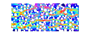
Particle trajectories  $\boldsymbol {x}(t) = [x(t),\kern-1.5pt y(t)]$ of different lengths and duration are recorded, along which velocities are sampled, and from which the displacement moments and propagators are determined. Figure 1 illustrates trajectories of non-motile and motile bacteria from the microfluidic experiments. We focus on displacements along the mean flow direction, which is aligned with the $x$-direction of the coordinate system. Particle displacements are calculated by
 \begin{equation} \Delta x(t_n) = x(t_0 + t_n) - x(t_0), \end{equation}
where  $x(t_0)$ is the starting position of the trajectory at time $t_0$ and $t_n = n \Delta t$ are subsequent sampling times. The time increment $\Delta t$ is given by the inverse frame rate of the camera. The displacement moments are determined by averaging over all particle trajectories
 \begin{equation} m_j(t_n) = \frac{1}{N_t} \sum_{k=1}^{N_t} \Delta x_k(t_n)^{j}, \end{equation}
where  $N_t$ denotes the number of tracks, and subscript $k$ denotes the $k$th trajectory. The displacement variance is defined in terms of the first and second displacement moments by
 \begin{equation} \sigma^2(t_n) = m_2(t_n) - m_1(t_n)^2. \end{equation}
The propagator or displacement distribution is defined by
 \begin{equation} p(x,\!t_n) = \frac{1}{N_t} \sum_{k=1}^{N_t} \frac{\mathbb{I}[x < \Delta x_k(t_n) \leq x + \Delta x ]}{\Delta x}, \end{equation}
where  $\mathbb {I}({\cdot })$ is the indicator function, which is $1$ if the argument is true and $0$ otherwise and $\Delta x$ is the size of the sampling bin. Note that the number of tracks decreases with track length and sampling time $t_n$, see the discussion in Appendix A. Table 1 provides a summary of the notation used in this paper.

Figure 1. Trajectories of motile bacteria at mean velocities (a,b)  $u_m = 98$ $\mathrm {\mu }$m s $^{-1}$ and (c,d) $u_m = 43$ $\mathrm {\mu }$m s $^{-1}$. The shaded area indicates the zoom in the right panel. The colour code corresponds to the local fluid velocities with respect to the mean. Velocity data were obtained by tracking passive particles in the flow.
Table 1. Notation.

2.2. Velocity statistics
Particle velocities  $\boldsymbol u(t) = [u_x(t),\kern-1.5pt u_y(t)]$ are obtained from the particle displacements between subsequent images
 \begin{equation} u_x(t) = \frac{x(t+\Delta t) - x(t)}{\Delta t},\quad u_y(t) = \frac{y(t+\Delta t) - y(t)}{\Delta t}. \end{equation}
The particle speed is defined by  $v(t) = \sqrt {u_x(t)^2 + u_y(t)^2}$. The mean particle velocity in the following is denoted by $\langle \boldsymbol {u}(t) \rangle = (u_m,0)$. The mean speed is denoted by $\langle v(t) \rangle = v_m$. Averages are taken over all tracks and sampling times. The speed probability density functions (PDFs) are obtained by sampling over all trajectories and sampling times.
Figure 2 shows the PDFs of particle speeds for the non-motile and motile bacteria, denoted by  $p_{nm}(v)$ and $p_m(v)$, respectively, rescaled by the mean speed $v_m$ of the non-motile bacteria. Non-motile bacteria can be considered passive tracer particles. Thus, the speed distributions of non-motile bacteria serve as a proxy for the Eulerian flow speed distribution, that is, $p_{nm}(v) \equiv p_e(v)$ which is supported by the fact that the rescaled data collapse on the same curve. The non-dimensional speed data are well represented by the gamma distribution
 \begin{equation} p_e(v) = \left(\frac{v \alpha}{v_m}\right)^{\alpha-1} \frac{\alpha \exp({-}v\alpha/v_m)}{v_m \varGamma(\alpha)}, \end{equation}
for  $\alpha = 2.25$. Speed distributions in porous media are often characterized by exponential or stretched exponential decay for $v > v_m$ and power-law behaviours at low flow speeds. Similar speed distributions have been reported in experimental particle tracking data (Holzner et al. Reference Holzner, Morales, Willmann and Dentz2015; Alim et al. Reference Alim, Parsa, Weitz and Brenner2017; Morales et al. Reference Morales, Dentz, Willmann and Holzner2017; Carrel et al. Reference Carrel, Morales, Dentz, Derlon, Morgenroth and Holzner2018; Souzy et al. Reference Souzy, Lhuissier, Méheust, Le Borgne and Metzger2020) and from numerical simulations of pore-scale flow (Siena et al. Reference Siena, Riva, Hyman, Winter and Guadagnini2014; Matyka, Golembiewski & Koza Reference Matyka, Golembiewski and Koza2016; De Anna et al. Reference De Anna, Quaife, Biros and Juanes2017; Aramideh, Vlachos & Ardekani Reference Aramideh, Vlachos and Ardekani2018; Dentz et al. Reference Dentz, Icardi and Hidalgo2018).

Figure 2. Speed distributions for (a) non-motile and (b) motile bacteria for different flow rates rescaled by the mean  $v_m$ of the respective non-motile speed distributions. The solid black lines in both panels denote the analytical approximation by the gamma distribution (2.6) of the speed distribution for the non-motile bacteria for $\alpha = 2.25$. The legend indicates the experiments, which are identified by the mean streamwise velocity of non-motile bacteria in $\mathrm {\mu }$m s $^{-1}$.
Panel (b) of figure 2 shows the speed PDFs for the motile bacteria rescaled by the mean speed of the respective non-motile bacteria, together with the gamma distribution given in (2.6), which models the non-motile speed PDFs. The global shapes of the rescaled speed PDFs for the motile bacteria are very similar to the speed PDF for the non-motile bacteria represented by the gamma distribution. However, they are shifted towards smaller values when compared with the non-motile bacteria, with a small peak at low values, which can be related to bacteria motion along the grains. The speed PDFs with  $u_m \geq 98$ $\mathrm {\mu }$m s $^{-1}$ scale with the mean speed $v_m$ and group together above all at those at intermediate and small speeds. The speed PDF of the motile bacteria measures the combined speed of the flow field and bacteria motility. The fact that the speed PDFs collapse when rescaled by the respective mean flow speeds indicates that bacteria motion scales with the flow speed. This seems to be different for the speed PDFs for $u_m \leq 66$ $\mathrm {\mu }$m s $^{-1}$. The PDFs are more scattered and shifted towards smaller values compared with the speed PDFs for the high flow rates.
Particle trajectories are tortuous due to pore and velocity structures, and thus are longer than the corresponding linear distance. The ratio between the average trajectory length of the non-motile bacteria and the linear length in the mean flow direction defines the tortuosity  $\chi$. It can be quantified by the ratio between the mean flow speed $v_m$ and the mean flow velocity $u_m$ as (Koponen, Kataja & Timonen Reference Koponen, Kataja and Timonen1996; Ghanbarian et al. Reference Ghanbarian, Hunt, Ewing and Sahimi2013; Puyguiraud, Gouze & Dentz Reference Puyguiraud, Gouze and Dentz2019b)
 \begin{equation} \chi = \frac{v_m}{u_m}. \end{equation}
We obtain from the velocity data at all flow rates tortuosity values between  $\chi = 1.17$ and $1.23$.
3. Theoretical approach
We present here the theoretical approach to modelling the dispersion of non-motile and motile bacteria. We use the CTRW framework to model the stochastic motion of bacteria due to pore-scale flow variability and motility, based on a spatial Markov model for subsequent particle velocities, and a compound Poisson process for motility. This type of approach was used to upscale and predict hydrodynamic transport in porous and fractured media at the pore and continuum scales (Berkowitz & Scher Reference Berkowitz and Scher1997; Noetinger et al. Reference Noetinger, Roubinet, Russian, Le Borgne, Delay, Dentz, de Dreuzy and Gouze2016; Dentz et al. Reference Dentz, Icardi and Hidalgo2018; Hyman et al. Reference Hyman, Rajaram, Srinivasan, Makedonska, Karra, Viswanathan and Srinivasan2019). It naturally accounts for the organization of the flow field along characteristic length scales that are imprinted in the host medium. We focus here on the quantification of the streamwise motion and large-scale dispersion of bacteria, which play a key role for the prediction of the length of bacteria plumes and the distributions of residence times in a porous medium.
3.1. Non-motile bacteria
Non-motile bacteria are considered as passive tracer particles that are transported by advection only. Non-motile bacteria move along streamlines of the pore-scale flow field, and thus explore the pore-scale velocity spectrum, except for the lowest velocities close to the grains, due to volume exclusion or molecular diffusion. Typical trajectories are shown in figure 1. In the following, we model the motion of non-motile bacteria using a spatial Markov model for particle speeds (Dentz et al. Reference Dentz, Kang, Comolli, Le Borgne and Lester2016; Morales et al. Reference Morales, Dentz, Willmann and Holzner2017; Puyguiraud et al. Reference Puyguiraud, Gouze and Dentz2019b).
3.1.1. Spatial Markov model
Particle motion is characterized by the spatial persistence of particle velocities over a characteristic length scale, which is imprinted in the spatial structure of the porous medium (Dentz et al. Reference Dentz, Kang, Comolli, Le Borgne and Lester2016). This provides a natural parameterization of bacteria motion in terms of travel distance. That is, motion is modelled by constant space and variable time increments along streamlines. Thus, the equations of streamwise motion of non-motile bacteria can be written as (Puyguiraud et al. Reference Puyguiraud, Gouze and Dentz2019b)
 \begin{equation} x_{n+1} = x_n + \frac{\Delta s}{\chi}, \quad t_{n+1} = t_n + \frac{\Delta s}{v_n}, \end{equation}
where  $\Delta s$ is the transition length along the tortuous particle path. The advective tortuosity $\chi$ accounts for streamline meandering in the pore space between the grains. It quantifies the ratio of the average streamline length to streamwise distance. Note that this meandering is different for each streamline and may be correlated with the particle speed. However, under ergodic flow conditions, the streamline lengths converge toward the average value and thus, at scales larger than $\ell _0$, tortuosity provides a good estimate for the longitudinal displacement.
The point distribution  $p_v(v)$ of particle speeds is given in terms of the Eulerian flow speed distribution $p_e(v)$
 \begin{equation} p_v(v) = \frac{v p_e(v)}{v_m}. \end{equation}
This speed-weighting relation is due to the fact that, in this framework, particles make transitions over constant distance, while the distribution of flow speeds  $p_e(v)$ is obtained by measuring speeds at constant frame rate, this means isochronically (Dentz et al. Reference Dentz, Kang, Comolli, Le Borgne and Lester2016; Morales et al. Reference Morales, Dentz, Willmann and Holzner2017; Puyguiraud et al. Reference Puyguiraud, Gouze and Dentz2019b). Equations (3.1a,b) constitute a CTRW because bacteria are propagated over constant (discrete) distances while time is a continuous variable. In this framework, the position $x(t)$ of a particle at time $t$ is given by $x(t) = x_{n_t}$, where $n_t = \max (n{|}t_n \leq t < t_{n+1})$. The displacement moments are defined by $m_i(t) = \langle x(t)^i \rangle$. The displacement variance is given by $\sigma ^2(t) = m_2(t) - m_1(t)^2$.
The series  $\{v_n\}$ of particle speeds is modelled as a stationary Markov process whose steady state distribution is given by (3.2). Specifically, we model $\{v_n\}$ through an Ornstein–Uhlenbeck process for the unit normal random variable $w_n$ which is obtained from $v_n$ through the transformation (Puyguiraud, Gouze & Dentz Reference Puyguiraud, Gouze and Dentz2019a)
 \begin{equation} w_n = \varPhi^{{-}1}[P_v(v_n)],\quad v_n = P_v^{{-}1}[\varPhi(w_n)], \end{equation}
where  $P_v$ is the cumulative speed distribution and $\varPhi ^{-1}(u)$ the inverse of the cumulative unit Gaussian distribution. Also, $w_n$ satisfies the Langevin equation
 \begin{equation} w_{n+1} = w_n - \ell_c^{{-}1} \Delta s w_n + \sqrt{2 \ell_c^{{-}1} \Delta s} \xi_n, \end{equation}
where  $\xi _n$ is a unit Gaussian random variable. The length scale $\ell _c$ denotes the characteristic correlation scale of particle speed. It is typically of the order of the characteristic grain size $\ell _0$ (Puyguiraud, Gouze & Dentz Reference Puyguiraud, Gouze and Dentz2021). However, its exact value needs to be adjusted from the data for the displacement variance. The increment $\Delta s$ is chosen such that $\Delta s \ll \ell _c$. The phase-space particle density $p(x,\kern-1.5pt v,\kern-0.09em t)$ in this framework is given by the Boltzmann-type equation (Comolli, Hakoun & Dentz Reference Comolli, Hakoun and Dentz2019)
 \begin{align} \frac{\partial p(x,\kern-1.5pt v,\kern-0.09em t)}{\partial t} + v \chi^{{-}1} \frac{\partial p(x,\kern-1.5pt v,\kern-0.09em t)}{\partial x} ={-} \frac{v}{\Delta s} p(x,\kern-1.5pt v,\kern-0.09em t) + \int_0^\infty {\rm d}v' r(v,\!\Delta s{|}v') \frac{v'}{\Delta s} p(x,\kern-1.5pt v'\!,\kern-1.4pt t), \end{align}
see also Appendix B.1. The initial distribution is given by  $p(x,\kern-1.5pt v,\kern-0.09em t = 0) = p_0(x,\kern-1.5pt v) = \delta (x) p_0(v)$, where $p_0(v)$ is the distribution of initial particle velocities. The propagator, that is, the distribution of particle displacements, is given by
 \begin{equation} p(x,\kern-0.09em t) = \int_0^\infty {\rm d}v p(x,\kern-1.5pt v,\kern-0.09em t). \end{equation}
3.1.2. Asymptotic theory
The behaviour of the upscaled model at travel distances much larger than the correlation length  $\ell _c$, can be obtained by coarse-graining particle motion on a length scale $\ell '_c \geq \ell _c$, such that
 \begin{equation} x_{n+1} = x_n + \frac{\ell'_c}{\chi}, \quad t_{n+1} = t_n + \tau_n. \end{equation}
The transition times  $\tau _n = \ell '_c/v_n$ are independent random variables whose distribution $\psi (t)$ is given in terms of $p_v(v)$ as
 \begin{equation} \psi(t) = \ell'_c t^{{-}2} p_v(\ell'_c/t) = \left(\frac{t}{\tau_0}\right)^{{-}2-\alpha} \frac{\exp(-\tau_0/t)}{\tau_0 \varGamma(\alpha+1)}, \end{equation}
where  $\tau _0 = \ell '_c/v_0$. $\psi (t)$ is given here by an inverse gamma distribution because the particle speed is gamma distributed, see (2.6).
For the velocity distribution (2.6) with  $\alpha = 2.25$, the CTRW predicts asymptotically a Fickian dispersion. That is, for times $t \gg \tau _v$, transport can be quantified by the advection–dispersion equation (Dentz & Berkowitz Reference Dentz and Berkowitz2003)
 \begin{equation} \frac{\partial p(x,\kern-0.09em t)}{\partial t} + u_m \frac{\partial p(x,\kern-0.09em t)}{\partial x} - D_{nm} \frac{\partial^2 p(x,\kern-0.09em t)}{\partial x^2} = 0, \end{equation}
with the average velocity  $u_m = v_m /\chi$ and the dispersion coefficient (Puyguiraud et al. Reference Puyguiraud, Gouze and Dentz2021)
 \begin{equation} D_{nm} = \frac{u_m \ell'_c}{2 \chi} \frac{\langle \tau^2 \rangle -\langle \tau \rangle^2}{\langle \tau \rangle^2}. \end{equation}
The mean and mean squared transition times are defined by
 \begin{equation} \langle \tau^k \rangle = \int_0^\infty {\rm d}t t^k \psi(t) = \tau_0^k \frac{\varGamma(\alpha + 1 - k)}{\varGamma(\alpha + 1)}, \end{equation}
for  $k = 1,2$. Here, $\varGamma (\alpha )$ denotes the gamma function. We find by comparison of the dispersion coefficients from the full spatial Markov model and the CTRW model (3.6a,b) that $\ell _c' \approx 1.57 \ell _c$.
3.2. Motile bacteria
We provide here the theoretical framework to interpret the trajectory data and motion of motile bacteria. The motion of motile bacteria is due to advection in the flow field and their own motility, as illustrated in figure 1. At zero flow rate, bacteria fluctuate in a random walk-like manner characterized by a zero mean displacement with a characteristic two-dimensional projected swimming velocity  $v_0 \approx 12$ $\mathrm {\mu }$m s $^{-1}$ (Creppy et al. Reference Creppy, Clément, Douarche, D'Angelo and Auradou2019). At finite flow rate, bacteria tend to swim along the streamlines, and make excursions perpendicular to them in order to move toward the solid grains. Based on the observations of Creppy et al. (Reference Creppy, Clément, Douarche, D'Angelo and Auradou2019) for bacteria motility, we couple the CTRW model for hydrodynamic transport with a trapping approach. These authors found that bacteria move towards the grains at a flow-dependent rate $\gamma$ and dwell on the grain surface for random times $\theta$, which are distributed according to the trapping time distribution $\psi _f(t)$.
3.2.1. Spatial Markov model and trapping
Within the CTRW approach outlined in the previous section, the trapping of bacteria is represented by a compound Poisson process for the time  $t_n$ of the bacteria after $n$ CTRW steps. Thus, the equations of motion are given by
 \begin{equation} x_{n+1} = x_n + \frac{\Delta s}{\chi}, \quad t_{n+1} = t_n + \frac{\Delta s}{v_n} + \tau(\Delta s/v_n), \end{equation}
for  $n >\! 1$. The initial displacement is $x_0 = 0$ for all bacteria. The initial time is set to $t_0 \!= 0$. The particle speeds $v_n$ evolve according to the process (3.3). The compound trapping time $\tau (r)$ is given by
 \begin{equation} \tau(r) = \sum_{i = 1}^{n_r} \theta_i, \end{equation}
where  $\theta _i$ is the trapping time associated with an individual trapping event, and $n_r$ is the number of trapping events during time $r$. The number of trapping events $n_r$ follows a Poisson process characterized by the rate $\gamma$, that is, the mean number of trapping events per CTRW step is $\gamma \Delta s/v_n$. The trapping rate is constant and counts the average number of trapping events per mobile time. While the trapping properties could depend, for example, on the local flow speeds, we use a Poisson process with constant rate as a robust and simple way of describing the average trapping properties, which is fully defined by the average number of trapping events per mobile time. The distribution of compound trapping times $\tau (r)$, denoted by $\psi _c(t{|}r)$, can be expressed in Laplace space by Feller (Reference Feller1968) and Margolin, Dentz & Berkowitz (Reference Margolin, Dentz and Berkowitz2003)
 \begin{equation} \psi_c^\ast(\lambda{|}r) = \exp(-\gamma r [1 - \psi^\ast_f(\lambda)] -\lambda r). \end{equation}
Here,  $\psi _c(t{|}r)$ denotes the probability that the trapping time is $t$ given that a trapping event occurred at time $r$. For $n = 1$, we distinguish the proportion $\rho$ of bacteria that are initially trapped, and $1 - \rho$ of initially mobile bacteria. For the trapped bacteria, $x_{1} = 0$ and $t_1 = \eta _0$, where the initial trapping time $\eta _0$ is distributed according to $\psi _0(t)$. For the mobile bacteria, $x_1$ and $t_1$ are given by (3.11a,b) for $n = 0$.
We consider here steady state conditions at time  $t = 0$. As experimental trajectories and their starting points are recorded continuously, it is reasonable to assume that a steady state between mobile and immobile bacteria is attained. Under steady state conditions, the joint probability of the bacteria being trapped and the initial trapping time being in $[t,t+{\rm d}t]$ is
 \begin{equation} \text{P}_0(t) = \int_t^\infty {\rm d}t' \gamma \exp[-\gamma (t' - t)] \psi_f(t'); \end{equation}
see Appendix C. The trapping times are assumed to be exponentially distributed, that is,
 \begin{equation} \psi_f(t) = \exp({-}t/\tau_c)/\tau_c, \end{equation}
with  $\tau _c$ the characteristic trapping time. This means we use Poissonian statistics to account for the effective retention of motile bacteria in the vicinity of grain surfaces. This picture is classically based on the idea that the run to tumble process promoting surface detachment is itself a memory-less Poisson process (Berg Reference Berg2018). However, there has been recent evidence that the run-time distribution for bacterial motion in a free fluid is a long-tail non-Poissonian process (Figueroa-Morales et al. Reference Figueroa-Morales, Soto, Junot, Darnige, Douarche, Martinez, Lindner and Clément2020b), which is also at the origin of long-tailed distributions of bacteria sojourn times on flat surfaces (Junot et al. Reference Junot, Darnige, Lindner, Martinez, Arlt, Dawson, Poon, Auradou and Clément2022). For porous media, there are currently no direct measurements that offer a quantitative microscopic description of the complex exchange processes taking place between the surface regions and the flowing regions. Thus, we adopt Poissonian statistics characterized by the mean retention time $\tau _c$ as a model with minimal assumptions. We hope that our conceptual approach, which provides a model of the emerging transport process, will motivate more detailed experimental investigations on this central question. Using (3.15) in (3.14), we obtain
 \begin{equation} \text{P}_0(t) = \frac{\beta}{1 + \beta} \frac{\exp({-}t/\tau_c)}{\tau_c}, \end{equation}
where we define the partition coefficient  $\beta = \gamma \tau _c$. Thus, the fraction of trapped bacteria is $\rho = \beta /(1 + \beta )$, and the initial trapping time distribution is $\psi _0(t) = \psi _f(t)$. Thus, the steady state partitioning of bacteria is directly related to their motility through the trapping rate $\gamma$ and mean dwelling time $\tau _c$ on the grain surface.
Note that this picture does not account for the tortuous particle path on the grain surfaces, which is represented as a localization event at fixed positions. Grain-scale bacteria motility could eventually be modelled by an additional process. However, here, we focus on large-scale bacteria dispersion and only account for tortuosity due to the flow path geometry. As above the bacteria position  $x(t)$ at time $t$ is given by $x(t) = x_{n_t}$. The expressions for the displacement mean and variance are analogous.
The density  $p_s(x,\kern-1.5pt v,\kern-0.09em t)$ of mobile bacteria in the stream is quantified by the non-local Boltzmann equation
 \begin{align} &\frac{\partial p_s(x,\kern-1.5pt v,\kern-0.09em t)}{\partial t} + \frac{\partial}{\partial t} \int_0^t {\rm d}t' \gamma \phi(t - t') p_s(x,\kern-0.09em t') + \frac{v}{\chi} \frac{\partial p_s(x,\kern-1.5pt v,\kern-0.09em t)}{\partial x} \nonumber\\ &\quad = \rho \delta(x) p_0(v) \psi_f(t) -\frac{v}{\Delta s} p_s(x,\kern-1.5pt v,\kern-0.09em t) + \int_0^\infty {\rm d}v' r(v{|}v') \frac{v'}{\Delta s} p_s(x,\kern-1.5pt v'\!,\kern-1.4pt t'), \end{align}
see Appendix B.2. We defined by
 \begin{equation} \phi(t) = \int_t^\infty {\rm d}t' \psi_f(t'), \end{equation}
the probability that the trapping time is larger than  $t$. Equation (3.17) reads as follows. The evolution of the particle density in the stream is given by the (second term on the left side) particle exchange between the stream and grain surface, (third term on the left) advection by the local velocity, (first term on the right side) release of bacteria that were initially on the grains and (second and third terms on the right) velocity transitions along the trajectory.
The total bacteria density is given by
 \begin{equation} p(x,\kern-1.5pt v,\kern-0.09em t) = p_s(x,\kern-1.5pt v,\kern-0.09em t) + p_g(x,\kern-1.5pt v,\kern-0.09em t). \end{equation}
The density  $p_g(x,\kern-1.5pt v,\kern-0.09em t)$ of bacteria on the grains is given by
 \begin{equation} p_g(x,\kern-1.5pt v,\kern-0.09em t) = \int_0^t {\rm d}t' \phi(t - t') \gamma p_s(x,\kern-1.5pt v,\kern-0.09em t') + \delta(x) \rho \phi(t) p_0(v). \end{equation}
This first term on the right side reads as follows. The density of bacteria on the grains is given by the probability per time  $\gamma p_s(x,\kern-0.09em t')$ that bacteria are trapped at time $t'$ times the probability $\phi (t - t')$ that the trapping time is longer than $t - t'$. The second term denotes the bacteria that are initially trapped and whose trapping time is larger than $t$. The speed $v$ associated with a bacteria on the grain should be understood as the bacteria speed before the trapping events.
3.2.2. Asymptotic theory
Similar to the discussion in the previous section for the non-motile bacteria, for distances much larger than  $\ell _c$, particle motion can be coarse grained such that
 \begin{equation} x_{n+1} = x_n + \ell'_c, \quad t_{n+1} = t_n + \tau_n+ \tau(\tau_n), \end{equation}
where the advective transition times  $\tau _n = \ell '_c/v_n$ are distributed according to (3.7). Here, $\tau (r)$ describes the compound Poisson process defined above. The propagator $p_s(x,\kern-0.09em t)$ of bacteria in the stream for this equation of motion is quantified by the non-local advection–dispersion equation
 \begin{align} &\frac{\partial p_s(x,\kern-0.09em t)}{\partial t} + \frac{\partial}{\partial t} \int_0^t {\rm d}t' \gamma \phi(t - t') p_s(x,\kern-0.09em t') \nonumber\\ &\quad + u_m \frac{\partial p_s(x,\kern-0.09em t)}{\partial x} - D_{nm} \frac{\partial^2 p_s(x,\kern-0.09em t)}{\partial x^2} = \rho \delta(x) \psi_f(t), \end{align}
while the distribution  $p_g(x,\kern-0.09em t)$ of bacteria at the grains is given by
 \begin{equation} p_g(x,\kern-0.09em t) = \int_0^t {\rm d}t' \phi(t - t') \gamma p_s(x,\kern-0.09em t') + \delta(x) \rho \phi(t). \end{equation}
Asymptotically, that is for times  $t \gg \tau _c$, the transport of the bacteria concentration $p(x,\kern-0.09em t)$ can be described by the advection–dispersion equation
 \begin{equation} \frac{\partial p_s(x,\kern-0.09em t)}{\partial t} + \frac{u_m}{R} \frac{\partial p_s(x,\kern-0.09em t)}{\partial x} - D_{m} \frac{\partial^2 p_s(x,\kern-0.09em t)}{\partial x^2} = 0, \end{equation}
see Appendix D. The retardation coefficient  $R$ and the asymptotic dispersion coefficient $D_{m}$ are given by the explicit expressions
 \begin{gather} R = 1 + \gamma \tau_c =\frac{1}{1-\rho}, \end{gather}
 \begin{gather} D_m = D_{nm} (1 - \rho) + u_m^2 \tau_c \rho (1-\rho)^2. \end{gather}
By definition,  $R$ compares the average velocity of motile bacteria with the average flow velocity. In the absence of trapping, $\rho =0$ and $R=1$, the bacteria are transported in the porous medium with an average velocity equal to the average fluid velocity. If trapping is present, retardation increases, indicating a decrease of the average bacteria velocity compared with the fluid velocity. The retardation coefficient is directly related to bacterial motility, which in our modelling framework is expressed by the trapping rate $\gamma$ and the mean retention time $\tau _c$ for which a bacteria dwells at the grain surface.
The asymptotic dispersion coefficient in (3.26) contains two terms. The first term  $D_{nm} (1-\rho )$ corresponds to the so-called dispersion coefficient at steady state (Yates, Yates & Gerba Reference Yates, Yates and Gerba1988; Tufenkji Reference Tufenkji2007). It predicts a reduction of the dispersion coefficient of the motile bacteria compared with the non-motile concomitant with the reduction of the average velocity of the bacteria population. It accounts for the dispersion of the motile proportion $1-\rho$ only. The second term quantifies a mechanism similar to Taylor dispersion. It originates from the spread of the bacteria plume due to fast transport in the pores and localization at the grains. The resulting dispersion effect can be rationalized as follows. The typical separation distance between localized and mobile bacteria, that is, the dispersion length is $u_m \tau _c$, while the dispersion time is $\tau _c$. The corresponding dispersion coefficient is the dispersion length squared divided by dispersion time, which gives exactly the scaling $u_m^2 \tau _c$ of (3.26). As we will see in the next section, this interaction can lead to a significant increase of bacteria dispersion compared with non-motile bacteria.
Asymptotic bacteria transport is predicted to obey the advection–dispersion equation with constant parameters for two reasons. First, the distribution of particle velocities does not tail towards low values, that is, the mean and mean squared transition times are finite. Second, the distribution of retention times is exponential. Thus, for times large compared with the characteristic mass transfer times, the support scale can be considered as well mixed, and, similar to Taylor dispersion (Taylor Reference Taylor1953), and generalized Taylor dispersion (Brenner & Edwards Reference Brenner and Edwards1993) transport can be described by an advection–dispersion equation.
4. Results
We discuss the experimental results for the displacement means and variances, as well as the displacement distributions, in the light of the theory presented in the previous section. As discussed in Appendix A, the number of experimentally observed tracks decreases with the travel time, which introduces a bias toward slower bacteria. Thus, in the following, we consider travel times shorter than  $5 \tau _v$ in order to avoid a too strong bias toward slow bacteria. Even so, as we will see below, there is a slowing down of the mean displacement with increasing travel time, specifically for the motile bacteria.
The proposed theoretical approach for the non-motile bacteria has one parameter that needs to be adjusted, the correlation scale  $\ell _c$, which typically is of the order of the grain size. It is adjusted here from the data for the displacement variance for the non-motile bacteria. The approach for the motile bacteria has two additional parameters, the trapping rate $\gamma$ and the mean trapping time $\tau _c$. The partition coefficient $\beta = \gamma \tau _c$ is adjusted from the mean displacement data for the motile bacteria, while the trapping time $\tau _c$ is adjusted from the data for the displacement variance of the motile bacteria. Thus, the non-motile CTRW model needs to adjust one parameter, which is of the order of the grain size. The motile CTRW model needs to adjust two parameters, which are related to the partitioning of bacteria between flowing and stagnant regions close to the grains.
4.1. Dispersion of non-motile bacteria
Figures 3 and 4 show displacement means and variances and the propagators for non-motile bacteria at different flow rates and for the same dimensionless times. Time is non-dimensionalized by the mean advection time over the size of a grain, which implies that the propagators are reported for the same mean travel distances. The CTRW model uses the velocity distribution (2.6) with  $\alpha = 2.25$, correlation length $\ell _c \approx 2 \ell _0$ and advective tortuosity $\chi = 1.2$.

Figure 3. (a) Normalized mean displacements and (b) normalized displacement variances for non-motile bacteria as a function of normalized time. The solid lines denote the estimate from the CTRW model. The dash-dotted line in the (b) indicates the initial ballistic growth.

Figure 4. Propagators of non-motile bacteria at (a–d)  $t = 0.1,0.9,2.6,4.3 \tau _v$. The blue solid lines denote the prediction of the CTRW model, the black lines are the fits from the Gaussian transport model that is characterized by the corresponding measured displacement mean and variance shown in figure 3.
The mean displacement is linear with a slightly higher slope at short compared with large times. It starts deviating from the expected behaviour  $m_1(t) = u_m t$ at around $t = 2 \tau _v$. We relate this behaviour to a bias due to the decrease in the number of tracks, as discussed in Appendix A. The displacement variance shows a ballistic behaviour at $t < \tau _v$, this means it increases as $t^2$. Then, for $t > \tau _v$, it increases superlinearly, which can be seen as a long cross-over to normal behaviour. These behaviours are accounted for by the CTRW model. For flow velocities $u_m \leq 66$ $\mathrm {\mu }$m s $^{-1}$, we observe a larger variance than for the higher flow rates. This, and the slightly smaller mean displacements compared to higher flow rates, can be attributed to the localization of some bacteria at the origin (see figure 4), which causes a chromatographic dispersion effect, which is discussed in more detail for the motile bacteria.
Figure 4 compares the experimental data for the propagators with the results of the CTRW model. The propagators are asymmetric but compact, meaning that there are no significant forward or backward tails in the distribution. For comparison, we plot a Gaussian-shaped propagator characterized by the mean displacement and displacement variance shown in figure 3. The asymmetry decreases with increasing travel time and the propagators become closer to the corresponding Gaussian. The CTRW model captures the initial asymmetry and the transition to symmetric Gaussian behaviour for all flow rates.
4.2. Dispersion of motile bacteria
Figures 5–7 show the displacement mean and variance, and the propagators for the motile bacteria at different flow rates. As in the previous section, time is measured in units of  $\tau _v$, that is, it measures the mean number of grains the bacteria have passed. The propagators are measured at the same non-dimensional times, that is, at the same mean distance. The motile CTRW model is parameterized by the same correlation length and tortuosity as the non-motile model. The partition coefficient $\beta = \gamma \tau _c$ is adjusted from the early time behaviour of the mean displacement, which is predicted to behave as
 \begin{equation} m_1(t) = \frac{u_m t}{R} = \frac{u_m t}{1 + \beta}, \end{equation}
because we consider the system to be initially in a steady state. The characteristic trapping time is adjusted from the displacement variance by keeping  $\beta$ fixed. We adjust $\tau _c = 2.5 \tau _v$ and $\beta = \gamma \tau _c = 0.4$ for $u_m \geq 98$ $\mathrm {\mu }$m s $^{-1}$, and $\tau _c = 2 \tau _v$ and $\beta = 1$ for $u_m = 66$ $\mathrm {\mu }$m s $^{-1}$.

Figure 5. (a) Normalized mean displacements and (b) normalized displacement variances for motile bacteria, as a function of normalized time. The experimental data are denoted by the symbols, the corresponding CTRW model results by the thick solid lines. The CTRW model uses  $\tau _c = 2.5 \tau _v$ and $\beta = \gamma \tau _c = 0.4$ for $u_m \geq 98$ $\mathrm {\mu }$m s $^{1}$ and $\tau _c = 2 \tau _v$ and $\beta = 1$ for $u_m = 66$ $\mathrm {\mu }$m s $^{1}$. The solid blue lines denote the model outcomes for the non-motile bacteria.

Figure 6. Distributions of motile bacteria for high flow rates at (a–d)  $t = 0.1$, 0.9, 2.6, $4.3\tau _v$. The blue solid lines denote the corresponding predictions of the CTRW model for the non-motile bacteria.

Figure 7. Propagators of motile bacteria for low flow rates at (a–d)  $t = 0.1$, 0.9, 2.6, $4.3 \tau _v$. The blue solid lines denote the prediction of the CTRW model for the non-motile bacteria.
As shown in figure 5, the mean displacement is consistently lower for the motile than for the non-motile bacteria, which is due to migration toward the grain surfaces and localization at the grains. The means displacement initially evolves linearly until a time of approximately  $2 \tau _v$ and, from there, the evolution slows down. We relate this to the decrease of the number of experimentally observed tracks, which induces a bias toward slow tracks, as discussed in Appendix A. In contrast to the mean displacement, the displacement variance can be larger than its non-motile counterpart for $u_m \geq 98$ $\mathrm {\mu }$m s $^{-1}$ and lower for $u_m \leq 66$ $\mathrm {\mu }$m s $^{-1}$. The data seem to fall into two groups for high and low flow rates, except for $u_m = 18$ $\mathrm {\mu }$m s $^{-1}$. In this case, the flow velocity is of the order of the swimming velocity $v_0 \approx 12$ $\mathrm {\mu }$m s $^{-1}$. The data indicate that that the density of trapped particles is higher at high compared with low flow rates. The possible mechanisms for these behaviours are discussed in § 5.
These behaviours are also reflected in the propagators shown in figure 6 for high flow rates with  $u_m \geq 98$ $\mathrm {\mu }$m s $^{-1}$ and in figure 7 for $u_m \leq 66$ $\mathrm {\mu }$m s $^{-1}$. The green symbols in figure 6 denote the experimental data rescaled by the mean grain size $\ell _0$, and the solid green lines the corresponding solution from the CTRW model for the parameters $\tau _c = 2.5 \tau _v$ and $\beta = \gamma \tau _c = 0.4$. Analogously, the red symbols in figure 7 denote the experimental data rescaled by the mean grain size $\ell _0$. The solid red lines show the corresponding solution from the CTRW model for the parameters $\tau _c = 2 \tau _v$ and $\beta = 1$. For comparison, we also plot the corresponding CTRW solution for the non-motile bacteria, marked by the blue solid lines. The motile propagators are delayed compared with the non-motile bacteria. They are characterized by a localized peak around zero and a pronounced forward tail, which can be attributed (i) to slow motion towards and around grains and (ii) to fast motion in the main pore channels. Figure 6 shows that the propagators at high flow rates ( $u_m \geq 98$ $\mathrm {\mu }$m s $^{-1}$) overlap, which indicates that bacteria motion scales with the mean flow. Similarly, for the low flow rates ( $u_m \leq 66$ $\mathrm {\mu }$m s $^{-1}$) shown in figure 7, we observe overlap in the forward tails, which are advection dominated due to transport in the pore channels. However, the upstream tails that develop starting from the localized peak do not group together. They can be attributed to bacteria motility, which is independent of the flow rate. This is most pronounced for $u_m = 18$ $\mathrm {\mu }$m s $^{-1}$, which is characterized by strong localization and an almost symmetric propagator. The features of peak localization and forward tailing show that a steady state in the macroscopic transport behaviour has not been attained at the largest observation time. At asymptotic times, that is, for $t \gg \tau _c$, the theoretical model given by (3.24) predicts Fickian transport characterized by symmetric propagators.
The data for the displacement moments and propagators seem to be grouped in two families, which we have highlighted by using two different colours. These observations are in agreement with the behaviours of the speed PDFs shown in figure 2. We therefore fit each family separately. From the early time evolution of the mean displacements, we adjust the partition coefficient  $\beta = 0.4$ for $u_m \geq 98$ $\mathrm {\mu }$m s $^{-1}$, $\beta = 1$ for $u_m \leq 66$ $\mathrm {\mu }$m s $^{-1}$. For $u_m \geq 98$ $\mathrm {\mu }$m s $^{-1}$, we adjust from the displacement data $\tau _c = 2.9 \tau _v$ and for $u_m = 66$ $\mathrm {\mu }$m s $^{-1}$, we adjust $\tau _c = 2.3 \tau _v$.
With these parameter sets, the CTRW model is able to describe the propagators and displacement moments as shown in figures 5 and 6. For the lowest flow velocity, bacteria are able to swim upstream over relatively long distances. The subsequent backward tail that develops because of the upstream motion is clearly visible in figure 6(c,d), and also, to a smaller extent, at the higher flow rates (a,b). This effect is not accounted for in the model that assumes that the trapping is localized and that trapped bacteria do not move once trapped.
Since  $\tau _v \propto 1/u_m$, our results indicate that the trapping rate increases linearly with the average flow velocity $u_m$ while the characteristic trapping time decreases linearly with $u_m$. We used different values for $\beta = \gamma \tau _v$ and $\tau _c$ to adjust the two sets. Recall that the fraction of trapped bacteria $\rho$ is $\beta /(1+\beta )$. Each set thus corresponds to a different value of the fraction of trapped bacteria. The fraction of trapped bacteria is high at low velocities ( $\rho \geq 0.5$) and decreases towards an asymptotic value of approximately $\rho = 0.3$ as the flow velocity is increased. The fraction of trapped bacteria is also related to the retardation coefficient $R$ through (3.25), which is estimated from the experimental data for the mean bacteria displacement according to relation (4.1). The dependence of $R$ and thus $\rho$ on the flow rate is further discussed in the next section.
4.3. Asymptotic dispersion and retardation
The CTRW model allows us to extrapolate the transport behaviours to times that cannot be reached in the experiment. Panels (a,b) of figure 8 show the displacement mean and variance up to times of  $1000 \tau _v$. We see that both observables evolve linearly at asymptotic times. The mean displacement indicates a lower average velocity for the motile than for the non-motile bacteria, which is due to trapping. The displacement variance on the other hand is larger for the motile than for the non-motile bacteria at high flow rates, which indicates stronger motile dispersion. This effect can be quantified by (3.25) and (3.26) for the retardation coefficient and asymptotic dispersion coefficient.

Figure 8. Model predictions for the displacement (a) means and (b) variances of motile and non-motile bacteria. (c) Retardation coefficient from experimental data. The dash-dotted line indicates the values used in the CTRW model at (green) high and (red) low flow rates. (d) Dispersion coefficient for the motile bacteria as a function of the fraction  $\rho$ of trapped bacteria for $\tau _c = 2 \tau _v, 2.5 \tau _v, 5 \tau _v$. The squares denote the dispersion coefficient at the $\rho$-values for (green square) $u_m \geq 98$ $\mathrm {\mu }$m s $^{-1}$ and (red square) $u_m = 66$ $\mathrm {\mu }$m s $^{-1}$.
The retardation coefficient  $R = 1/(1-\rho ) = 1+ \beta$ can be estimated directly from the experimental data for the mean displacement according to (4.1). Panel (c) of figure 8 shows that the retardation coefficient decreases with increasing flow rate, which is consistent with the values adjusted for $\beta$ in the previous section. Thus the data show also that the fraction $\rho$ of trapped particles decreases with increasing flow rate.
The behaviour of  $D_m$ as a function of the proportion $\rho$ of trapped bacteria is shown in panels (c,d) of figure 8. The solid line shows the theoretical behaviour of $D_{nm}$ for $\tau _c = 2.5\tau _v$ and $\tau _c = 2 \tau _v$, which corresponds to the value used in the CTRW model. The green and red symbols denote the values obtained from the CTRW models at high and low flow rates. We see that, at low fractions of immobile bacteria, the Taylor term in (3.26) dominates and motile bacteria disperse more than non-motile. At high proportions of trapped bacteria, localization dominates over the Taylor mechanism, and motile dispersion is lower than non-motile. Figure 8 illustrates the competition between the trapping time $\tau _c$ and the proportion $\rho$ of trapped bacteria. For increasing $\tau _c$, motile dispersion can be significantly larger than non-motile dispersion.
5. Discussion
We study the interaction between bacteria motility and flow variability, and its impact on the dispersion of bacteria. To do so we use data obtained in a microfluidic chip containing randomly placed obstacles, in which thousands of non-motile and motile bacteria were tracked at different flow rates. This geometry reproduces the structure of a porous medium on the scale of a few pores, and is thus ideal to study transport phenomena at the pore scale. Because bacteria do not adhere to the surface of the flow cell, this set-up allows us to study the first step of filtration, which consists of the transport of bacteria from the flowing fluid to regions of low flow in the vicinity of solid grains.
Bacteria motion is quantified by a CTRW approach that is based on a Markov model for equidistant particle speeds. The experimental data for the displacement of non-motile bacteria are used to constrain the velocity correlation length, which is of the order of the grain size. Bacteria motility is modelled in this framework by a trapping process, which accounts for the rheotactic motion toward and along the grain surfaces by a trapping rate  $\gamma$ and characteristic dwelling time $\tau _c$. The ratio between trapped and mobile bacteria at steady state is measured by the partition coefficient $\beta = \gamma \tau _c$.
Adjustment of the model to the experimental data reveals two main features. Firstly, we observe that  $\gamma \propto u_m$ and $\tau _c \propto 1/u_m$. The increase of the trapping rate with the flow rate can be explained by the constant reorientation of the bacteria by the flow. The frequency at which bacteria point toward the grains increases with the flow rate, which may explain the increase of the trapping rate. Similarly, for increasing flow rate, shear increases on the grains and thus the area for motion around the grains decreases and the bacteria are more easily blown off by the flow. This can explain why the residence time decreases with flow rate. A model that supports this idea is proposed in Appendix E.
Secondly, we observe that the ratio  $\beta$ between trapped and mobile bacteria is different at high and low flow rates. This observation indicates a transition between a regime at low flow rates, where motility favours trapping with a high density of trapped bacteria (approximately $50\,\%$ of trapped bacteria), to a regime at high flow rates, where the flow hinders trapping (approximately $30\,\%$ of trapped bacteria). Two phenomena may contribute to this change. The first comes from the volume of fluid in which the bacteria can be considered as trapped. This fraction can be separated in two: a part where the velocity is very small (this part corresponds to the dark blue regions that can be seen in figure 1 and is always present for all the flow rates used) and a second contribution which comes from the regions of flowing fluid where the average flow velocity is less than the swimming velocity. In those volumes, which are located close to the grain surface, the bacteria trajectories are little influenced by the flow and they swim much as in a quiescent fluid. Bacteria can be considered trapped when they swim along the grain surfaces. This contribution, however, decreases with the flow rate, reducing in turn the density of trapped bacteria, as observed. The second contribution comes from the diffusion due to the constant reorientation of the bacteria. In a fluid at rest, the trajectories of the bacteria can be decomposed into a succession of runs followed by tumbles that reorient the bacteria. At large scale, the reorientation is diffusive and can be characterized by the translational diffusion coefficient $D_b$. For E. coli we have here $D_b \approx 243$ $\mathrm {\mu }$m $^2$ s $^{-1}$ (Creppy et al. Reference Creppy, Clément, Douarche, D'Angelo and Auradou2019). In a shear flow, bacteria constantly tumble and are reoriented at a frequency set be the shear rate $\dot {\gamma }$ (Jeffery Reference Jeffery1922). When the Péclet number defined as $Pe = u_m \ell _0/{2 D_b}$ is of the order of $1$ and for a grain size of $\ell _0 = 30$ $\mathrm {\mu }$m, we have $Pe \simeq u_m/(16$ $\mathrm {\mu }$m s $^{-1}$). Random orientation will thus dominate shear alignment for the lowest flow rate with little or no influence at high flow velocity.
6. Conclusions
In conclusion, to understand the dispersion of bacteria in porous media, our study focuses on the central importance of hydrodynamic flow fluctuations and the active exploration process into high shear regions around the solid grains. The rheotactic coupling between flow and bacteria motility manifests itself at intermediate scales through non-Fickian behaviour, and at large scales through a motility-dependent hydrodynamic dispersion effect. Noticeably, the interplay between fast transport in the flow and motile motion toward grain surfaces is the first necessary step before possible adhesion (Yates et al. Reference Yates, Yates and Gerba1988). To date, it had been assumed that the transfer between regions of high fluid flow and low flow regions in the vicinity of the grain surfaces was diffusive, as for passive solutes, and had been modelled as a kinetic single-rate mass transfer process (Yates et al. Reference Yates, Yates and Gerba1988; Bai et al. Reference Bai, Cochet, Pauss and Lamy2016). Our study suggests that both motility and flow play a central role in the trapping and release processes, which are characterized by two different rates. Both trapping and release rates are proportional to the average flow velocity, while the ratio between mobile and trapped bacteria increases with increasing flow velocity. The trapping and release mechanisms explain apparently contradictory observations of the concomitant enhancement of retention and dispersion. They are quantified in a theoretical approach that captures the salient features of the experimental displacement data, and allows for prediction of the dispersion of motile bacteria at large scales. These findings shed light on the strategies microorganisms may use to maximize their survival and proliferation abilities under natural conditions, and can give new insights into bacteria filtration and biofilm growth, for which the contact with grain surfaces is determinant.
Funding
M.D. acknowledges the support of the Spanish Research Agency (10.13039/501100011033) and the Spanish Ministry of Science and Innovation through the grants CEX2018-000794-S and PID2019-106887GB-C31 (HydroPore). H.A and C.D. acknowledge the support of the ‘Laboratoire d'Excellence Physics Atom Light Mater’ (LabEx PALM) as part of the ‘Investissements d'Avenir’ program (reference: ANR-10-LABX-0039). E.C., H.A., C.D. and A.C. are supported by the ANR grant ‘BacFlow’ ANR-15-CE30-0013. E.C. is supported by the Institut Universitaire de France.
Declaration of interests
The authors report no conflict of interest.
Appendix A. Track length statistics
The number of observed tracks decreases with time because tracks leave the observation window according to their average velocity. Figure 9 shows the number of tracks of non-motile and motile bacteria for the experiments at different flow rates as a function of time measured in units of the characteristic advection time  $\tau _v$, which here is the time to move over the characteristic grain length $\ell _0$ by mean advection $u_m$. We see that the number of tracks decreases to around $90\,\%$ of the initial number of tracks after around $2 \tau _v$ for the non-motile and motile bacteria. After around $4 \tau _v$ the number of tracks decreases to approximately $35\,\%$ for the non-motile and to around $40\,\%$ for the motile bacteria. This means that the number of tracks of lengths larger than $4 \ell _0$ is $35\,\%$ and $40\,\%$ of the total number of tracks. The long tracks are tortuous low velocity tracks that can be observed for a longer time. This is supported by the observation that the mean velocity starts decreasing after approximately $2 \tau _v$, as shown in figures 3 and 5 below. In the following, we consider travel times shorter than $5 \tau _v$ in order to avoid too strong a bias toward slow bacteria. Even so, as we will see below, there is a significant slowing down of the mean displacement with increasing travel time, specifically for the motile bacteria.

Figure 9. Number of tracks of (a) non-motile and (b) motile bacteria as a function of time.
Appendix B. CTRW model
The streamwise motion of a non-motile bacteria in the CTRW is described by (3.1a,b). Unlike classical random walk strategies for the modelling of particle motion in heterogeneous flow fields, the CTRW approach models particle motion based on stochastic series of equidistant instead of isochronic particle speeds (e.g. Dentz et al. Reference Dentz, Kang, Comolli, Le Borgne and Lester2016; Morales et al. Reference Morales, Dentz, Willmann and Holzner2017), that is, particle speeds that change at equidistant points along a streamline. The streamwise displacement in the CTRW model represents the projection of the tortuous streamline onto the mean flow direction using advective tortuosity  $\chi$. This is illustrated schematically in figure 10.

Figure 10. Schematic of the representation of a particle trajectory in the CTRW approach. Particle speeds are sampled equidistantly at turning points along a trajectory indicated by the constant  $\Delta s$. The CTRW represents the trajectory projected onto the direction of the mean flow.
B.1. Non-motile bacteria
In the following, we provide a derivation of the Boltzmann-type equation (3.4) for the joint distribution  $p(x,\kern-1.5pt v,\kern-0.09em t)$ of bacteria displacement and speed. For more details, see Comolli et al. (Reference Comolli, Hakoun and Dentz2019). The distribution $p(x,\kern-1.5pt v,\kern-0.09em t)$ can be written as
 \begin{equation} p(x,\kern-1.5pt v,\kern-0.09em t) = \int_0^t {\rm d}t' R(x,\kern-1.5pt v,\kern-0.09em t') \int_{t-t'}^\infty {\rm d}t'' \psi(t{|}v), \end{equation}
where  $\psi (t{|}v) = \delta (t - \Delta s/v)$. The probability per time $R(x,\kern-1.5pt v,\kern-0.09em t)$ for the particle to just arrive at $(x,\kern-1.5pt v)$ at $t$ satisfies
 \begin{equation} R(x,\kern-1.5pt v,\kern-0.09em t) = R_0(x,\kern-1.5pt v,\kern-0.09em t) + \int_0^t {\rm d}t' \int {\rm d} x' \int {\rm d}v' \psi(x-x',\kern-0.09em t-t'{|}v') r(v{|}v') R(x',\kern-0.09em v',\kern-0.09em t'), \end{equation}
where  $r(v{|}v')$ is the transition probability from $v'$ to $v$, and
 \begin{equation} \psi(x,\kern-0.09em t{|}v) = \delta(x - \Delta s/\chi) \delta(t - \Delta s/v). \end{equation}
The initial condition is encoded in  $R_0(x,\kern-1.5pt v,\kern-0.09em t)$, which is defined by
 \begin{equation} R_0(x,\kern-1.5pt v,\kern-0.09em t) = p_0(x,\kern-1.5pt v) \delta(t), \end{equation}
where  $p_0(x,\kern-1.5pt v)$ is the distribution of initial particle positions and speeds. Equations (B1a) and (B1b) can be combined in Laplace space to the generalized master equation
 \begin{align} \lambda p^\ast(x,\kern-1.5pt v,\kern-0.09em \lambda) &= R_0^\ast(x,\kern-1.5pt v,\kern-0.09em \lambda)+ \int {\rm d} x' \int {\rm d}v' r(v{|}v')\nonumber\\ &\quad \times \left[\frac{\lambda \psi^\ast(x-x',\kern-0.09em \lambda{|}v')}{1 - \psi^\ast(\lambda{|}v')} p^\ast(x',\kern-0.09em v',\kern-0.09em \lambda) - \frac{\lambda \psi^\ast(\lambda{|}v)}{1 - \psi^\ast(\lambda{|}v)} p^\ast(x,\kern-1.5pt v,\kern-0.09em \lambda)\right]. \end{align}
Using the explicit form (B2) for  $\psi (x,\kern-0.09em t{|}v)$, it can be written as
 \begin{align} \lambda p^\ast(x,\kern-1.5pt v,\kern-0.09em \lambda) &= R_0^\ast(x,\kern-1.5pt v,\kern-0.09em \lambda) + \int {\rm d}v' r(v{|}v') \frac{\lambda \exp(-\lambda \Delta s/v')}{1 - \exp(-\lambda \Delta s/v')} p^\ast(x - \Delta s/\chi,\kern-1.4pt v',\kern-0.09em \lambda)\nonumber\\ &\quad - \frac{\lambda \exp(-\lambda \Delta s/v)}{1 - \exp(-\lambda \Delta s/v)} p^\ast(x,\kern-1.5pt v,\kern-0.09em \lambda). \end{align}
In the limit of  $\Delta s \ll \ell _c$, we can write
 \begin{align} &\lambda p^\ast(x,\kern-1.5pt v,\kern-0.09em \lambda) \nonumber\\ &\quad =R_0^\ast(x,\kern-1.5pt v,\kern-0.09em \lambda) + \int {\rm d}v' r(v{|}v') \left[\frac{v'}{\Delta s} p^\ast(x - \Delta s/\chi,\kern-1.4pt v',\kern-0.09em \lambda) - \frac{v}{\Delta s} p^\ast(x,\kern-1.5pt v,\kern-0.09em \lambda)\right]\nonumber\\ &\quad = R_0^\ast(x,\kern-1.5pt v,\kern-0.09em \lambda) + \int {\rm d}v' r(v{|}v') \frac{v'}{\Delta s} p^\ast(x,\kern-1.5pt v',\lambda) - \frac{v}{\chi} \frac{\partial}{\partial x} p^\ast(x,\kern-1.5pt v,\kern-0.09em \lambda) - \frac{v}{\Delta s} p^\ast(x,\kern-1.5pt v,\kern-0.09em \lambda), \end{align}
where we localized  $r(v{|}v') = \delta (v-v')$ in the advection term. By transformation back to time, we obtain the Boltzmann equation
 \begin{equation} \frac{\partial p(x,\kern-1.5pt v,\kern-0.09em t)}{\partial t} + \frac{v}{\chi} \frac{\partial p(x,\kern-1.5pt v,\kern-0.09em t)}{\partial x} ={-}\frac{v}{\Delta s} p(x,\kern-1.5pt v,\kern-0.09em t) + \int_0^\infty {\rm d}v' r(v{|}v') \frac{v'}{\Delta s} p(x,\kern-1.5pt v'\!,\kern-1.4pt t'). \end{equation}
B.2. Motile bacteria
In the case of motile bacteria, we account for trapping during advective steps as well as initial trapping. Thus, we modify (B1) as
 \begin{equation} p(x,\kern-1.5pt v,\kern-0.09em t) = \int_{0}^t {\rm d}t' R_0(x,\kern-1.5pt v,\kern-0.09em t') \int_{t-t'}^\infty {\rm d}t' \psi_0(t{|}v) + \int_0^t {\rm d}t' R(x,\kern-1.5pt v,\kern-0.09em t') \int_{t-t'}^\infty {\rm d}t'' \psi_c(t{|}v). \end{equation}
We define the initial transition probability
 \begin{equation} \psi_0(x,\kern-0.09em t{|}v) = (1-\rho) \delta(x - \Delta s) \psi_c(t{|}v) + \rho \delta(x) \psi_f(t{|}v), \end{equation}
and the distribution of initial transition times
 \begin{equation} \psi_0(t{|}v) = \int {\rm d} x \psi_0(x,\kern-0.09em t{|}v) = (1-\rho) \psi_c(t{|}v) + \rho \psi_f(t{|}v). \end{equation}
The distribution of compound transition times is given by
 \begin{equation} \psi_c(t{|}v) = \int_0^t {\rm d}t' \psi(t'{|}v) \psi_c(t-t'{|}t'), \end{equation}
where  $\psi _c(t-t'{|}t')$ is defined by (3.13). This relation reads in Laplace space as
 \begin{equation} \psi_c^\ast(\lambda{|}v) = \psi^\ast(\lambda[1 - \gamma \psi_f^\ast(\lambda)]) = \exp(-\lambda[1 - \gamma \psi_f^\ast(\lambda)] \Delta s/v). \end{equation}
The probability per time  $R(x,\kern-1.5pt v,\kern-0.09em t)$ for the particle to just arrive at $(x,\kern-1.5pt v)$ at $t$ satisfies
 \begin{equation} R(x,\kern-1.5pt v,\kern-0.09em t) = R_1(x,\kern-1.5pt v,\kern-0.09em t) + \int_0^t {\rm d}t' \int {\rm d} x' \int {\rm d}v' \psi_c(x-x',\kern-0.09em t-t'{|}v') r(v{|}v') R(x',\kern-0.09em v',\kern-0.09em t'), \end{equation}
where  $r(v{|}v')$ is the transition probability from $v'$ to $v$, and
 \begin{equation} \psi_c(x,\kern-0.09em t{|}v) = \delta(x - \Delta s) \psi_c(t{|}v). \end{equation}
The function  $R_1(x,\kern-1.5pt v,\kern-0.09em t)$ is given by
 \begin{equation} R_1(x,\kern-1.5pt v,\kern-0.09em t) = \int_0^t {\rm d}t' \int {{\rm d}\kern0.05em x}' \int {\rm d}v' \psi_0 (x-x',\kern-0.09em t-t'{|}v') r(v{|}v') R_0(x',\kern-0.09em v',\kern-0.09em t'). \end{equation}
Equations (B8a) and (B8f) can be combined in Laplace space to the generalized master equation
 \begin{align} \lambda G^\ast(x,\kern-1.5pt v,\kern-0.09em \lambda) &= R_1^\ast(x,\kern-1.5pt v,\kern-0.09em \lambda) + \int {\rm d}v' r(v{|}v') \frac{\lambda \psi_c^\ast(\lambda{|}v')}{1-\psi_c^\ast(\lambda{|}v')} G^\ast(x - \Delta s/\chi,\kern-1.4pt v',\kern-0.09em \lambda)\nonumber\\ &\quad - \frac{\lambda \psi_c^\ast(\lambda{|}v)}{1-\psi_c^\ast(\lambda{|}v)} G^\ast(x,\kern-1.5pt v,\kern-0.09em \lambda), \end{align}
where we defined
 \begin{equation} G^\ast(x,\kern-1.5pt v,\kern-0.09em \lambda) = \left[p^\ast(x,\kern-1.5pt v,\kern-0.09em \lambda) - R_0^\ast(x,\kern-1.5pt v,\kern-0.09em \lambda) \frac{1 - \psi_0(\lambda{|}v)}{\lambda} \right]. \end{equation}
Using this definition and definition (B10), we can write (B11) as
 \begin{align} &\lambda p^\ast(x,\kern-1.5pt v,\kern-0.09em \lambda) = R_0^\ast(x,\kern-1.5pt v,\kern-0.09em\lambda)\nonumber\\ &\quad +\int {\rm d} x' \int {\rm d}v' r(v{|}v') \left[ \psi_0^\ast (x-x',\lambda{|}v') R_0^\ast(x',\kern-0.09em v',\kern-0.09em \lambda) - \psi_0^\ast(\lambda{|}v) R_0^\ast(x,\kern-1.5pt v,\kern-0.09em \lambda) \right]\nonumber\\ &\quad + \int {\rm d}v' r(v{|}v') \left[\frac{\lambda \psi_c^\ast(\lambda{|}v')}{1-\psi_c^\ast(\lambda{|}v')} G^\ast(x - \Delta s/\chi,\kern-1.4pt v',\kern-0.09em \lambda) - \frac{\lambda \psi_c^\ast(\lambda{|}v)}{1-\psi_c^\ast(\lambda{|}v)} G^\ast(x,\kern-1.5pt v,\kern-0.09em \lambda)\right]. \end{align}
Using the definition (B8b) of  $\psi _0(x,\kern-0.09em t{|}v)$, we obtain
 \begin{align} &\lambda p^\ast(x,\kern-1.5pt v,\kern-0.09em \lambda) = R_0^\ast(x,\kern-1.5pt v,\kern-0.09em \lambda)\nonumber\\ &\quad + \int {\rm d} x' \int {\rm d}v' r(v{|}v') (1 - \rho) [\psi_c^\ast (\lambda{|}v') R_0^\ast(x - \Delta s/\chi,\kern-1.4pt v',\kern-0.09em \lambda) - \psi_c^\ast(\lambda{|}v) R_0^\ast(x,\kern-1.5pt v,\kern-0.09em \lambda) ]\nonumber\\ &\quad + \int {\rm d}v' r(v{|}v') \left[\frac{\lambda \psi_c^\ast(\lambda{|}v')}{1-\psi_c^\ast(\lambda{|}v')} G^\ast(x - \Delta s/\chi,\kern-1.4pt v',\kern-0.09em \lambda) - \frac{\lambda \psi_c^\ast(\lambda{|}v)}{1-\psi_c^\ast(\lambda{|}v)} G^\ast(x,\kern-1.5pt v,\kern-0.09em \lambda)\right]. \end{align}
Note that
 \begin{align} &\frac{\lambda \psi_c^\ast(\lambda{|}v)}{1-\psi_c^\ast(\lambda{|}v)} R_0^\ast(x,\kern-1.5pt v,\kern-0.09em \lambda) \frac{1 - \psi_0(\lambda{|}v)}{\lambda}\nonumber\\ &\quad = R_0^\ast(x,\kern-1.5pt v,\kern-0.09em \lambda) (1 - \rho) \psi_c^\ast(\lambda{|}v) + \rho R_0^\ast(x,\kern-1.5pt v,\kern-0.09em \lambda) \frac{\psi_c^\ast(\lambda{|}v)}{1-\psi_c^\ast(\lambda{|}v)} \phi^\ast(\lambda), \end{align}
where we defined
 \begin{equation} \phi^\ast(\lambda) = \frac{1 - \psi^\ast_f(\lambda)}{\lambda}. \end{equation}
Combining everything, we obtain
 \begin{align} \lambda p^\ast(x,\kern-1.5pt v,\kern-0.09em \lambda) &= R_0^\ast(x,\kern-1.5pt v,\kern-0.09em \lambda) + \int {\rm d}v' r(v{|}v') \frac{\lambda \psi_c^\ast(\lambda{|}v')}{1-\psi_c^\ast(\lambda{|}v')} G_m^\ast( x - \Delta s/\chi,\kern-1.4pt v',\kern-0.09em \lambda) \nonumber\\ &\quad - \frac{\lambda \psi_c^\ast(\lambda{|}v)}{1-\psi_c^\ast(\lambda{|}v)} G_m^\ast(x,\kern-1.5pt v,\kern-0.09em \lambda), \end{align}
where we defined
 \begin{equation} G^\ast_m(x,\kern-1.5pt v,\kern-0.09em \lambda) = p^\ast(x,\kern-1.5pt v,\kern-0.09em \lambda) - \rho R_0^\ast(x,\kern-1.5pt v,\kern-0.09em \lambda) \phi^\ast(\lambda). \end{equation}
Furthermore, we approximate for small  $\Delta s$
 \begin{equation} \frac{\psi_c^\ast(\lambda{|}v)}{1-\psi_c^\ast(\lambda{|}v)} = \frac{v}{\Delta s} \frac{1}{1+\gamma \phi^\ast(\lambda)}. \end{equation}
Thus, we obtain
 \begin{align} \lambda p^\ast(x,\kern-1.5pt v,\kern-0.09em \lambda) &= R_0^\ast(x,\kern-1.5pt v,\kern-0.09em \lambda) + \int {\rm d}v' r(v{|}v') \frac{v'}{\Delta s} \frac{G_m^\ast(x - \Delta s/\chi,\kern-1.4pt v',\kern-0.09em \lambda)}{1+\gamma \phi^\ast(\lambda)}\nonumber\\ &\quad - \frac{v}{\Delta s} \frac{G_m^\ast(x,\kern-1.5pt v,\kern-0.09em \lambda)}{1+\gamma \phi^\ast(\lambda)}. \end{align}
We define now the mobile concentration of bacteria in the stream as
 \begin{equation} p_s^\ast(x,\kern-1.5pt v,\kern-0.09em \lambda) = \frac{G_m^\ast(x,\kern-1.5pt v,\kern-0.09em \lambda)}{1+\gamma \phi^\ast(\lambda)} = \frac{p^\ast(x,\kern-1.5pt v,\kern-0.09em \lambda) - \rho R_0^\ast(x,\kern-1.5pt v,\kern-0.09em \lambda) \phi^\ast(\lambda)}{1+\gamma \phi^\ast(\lambda)}. \end{equation}
With this definition, we obtain
 \begin{align} &\lambda [1 + \gamma \phi^\ast(\lambda)] p_s^\ast(x,\kern-1.5pt v,\kern-0.09em \lambda) = R_0^\ast(x,\kern-1.5pt v,\kern-0.09em \lambda) - \rho \lambda R_0^\ast(x,\kern-1.5pt v,\kern-0.09em \lambda) \phi^\ast(\lambda)\nonumber\\ &\quad + \int {\rm d}v' r(v{|}v') \left[\frac{v'}{\Delta s} p_s^\ast(x - \Delta s/\chi,\kern-1.4pt v',\kern-0.09em \lambda) - \frac{v}{\Delta s} p_s^\ast(x,\kern-1.5pt v,\kern-0.09em \lambda) \right]. \end{align}
Expanding the integral terms on the right side in analogy to the previous section gives
 \begin{align} &\lambda [1 + \gamma \phi^\ast(\lambda)] p_s^\ast(x,\kern-1.5pt v,\kern-0.09em \lambda) = R_0^\ast(x,\kern-1.5pt v,\kern-0.09em \lambda) - \rho \lambda R_0^\ast(x,\kern-1.5pt v,\kern-0.09em \lambda) \phi^\ast(\lambda)\nonumber\\ &\quad + \int {\rm d}v' r(v{|}v') \frac{v'}{\Delta s} p_s^\ast(x,\kern-1.5pt v',\kern-1.5pt \lambda) - \frac{v}{\chi} \frac{\partial}{\partial x} p_s^\ast(x,\kern-1.5pt v,\kern-0.09em \lambda) - \frac{v}{\Delta s} p_s^\ast(x,\kern-1.5pt v,\kern-0.09em \lambda). \end{align}
By transformation back to time, we obtain the Boltzmann equation
 \begin{align} &\frac{\partial p_s(x,\kern-1.5pt v,\kern-0.09em t)}{\partial t} + \frac{\partial}{\partial t} \int_0^t {\rm d}t' \gamma \phi(t - t') p_s(x,\kern-0.09em t') + \frac{v}{\chi} \frac{\partial p_s(x,\kern-1.5pt v,\kern-0.09em t)}{\partial x} \nonumber\\ &\quad = \rho p_0(x,\kern-1.5pt v) \psi_f(t) -\frac{v}{\Delta s} p_s(x,\kern-1.5pt v,\kern-0.09em t) + \int_0^\infty {\rm d}v' r(v{|}v') \frac{v'}{\Delta s} p_s(x,\kern-1.5pt v'\!,\kern-1.4pt t'). \end{align}
Appendix C. Initial trapping time distribution
In order to derive the initial trapping time distribution, we employ the concept of the backward recurrence time  $B_{t_0} = t_0 - t_N$, this means the time that has passed between a target time $t_0$ and the time $t_N$ of the last trapping event before $t_0$. For a Poissonian trapping process, this means that, for an exponential inter-event time distribution, the distribution of $B_{t_0}$ in the steady state limit, that is, for $N \to \infty$, is given by (Godrèche & Luck Reference Godrèche and Luck2001)
 \begin{equation} \psi_B(t) = \gamma \exp(-\gamma t). \end{equation}
It is independent from  $t_0$, $B_{t_0} \equiv B$. The initial trapping time $\eta _0$ can be expressed in terms of $B$ as $\eta _0 = \tau _f - B$. Thus, the joint distribution for a bacteria to be trapped and have the trapping time $\eta _0 < t$ is
 \begin{equation} \text{Prob}(\eta_0 < t \land \text{trapped}) = \left\langle H(\tau_f - B) H[t - (\tau_f - B)] \right\rangle \end{equation}
It can be written as
 \begin{equation} \text{Prob}(\eta_0 < t \land \text{trapped}) = \int_0^\infty {\rm d}t' \int_{0}^\infty {\rm d} t'' H(t' - t'') H[t - (t' - t'')] \psi_B(t'') \psi_f(t'). \end{equation}
Using expression (C1) for  $\psi _B(t)$ and shifting $t'' \to t' -t''$, we obtain
 \begin{align} \text{Prob}(\eta_0 < t \land \text{trapped}) &= \int_0^\infty {\rm d}t' \int_{0}^{\infty} {\rm d} t'' \gamma \exp[-\gamma (t'-t'')] \psi_f(t') H(t - t'') H(t'-t'') \nonumber\\ &= \int_0^t {\rm d}t'' \int_{t''}^{\infty} {\rm d} t' \gamma \exp[-\gamma (t'-t'')] \psi_f(t'). \end{align}
Thus, we obtain for the joint probability of being trapped and  $\eta _0$ in $[t,t+{\rm d}t]$ by derivation of (C4) with respect to $t$
$t$
 \begin{equation} \text{P}_0(t) = \int_{t}^{\infty} {\rm d} t' \gamma \exp[-\gamma (t'-t)] \psi_f(t'). \end{equation}
For  $\psi _f(t) = \exp (-t/\tau _c)/\tau _c$, we obtain
 \begin{align} \text{Prob}(\eta_0 < t \land \text{trapped}) &= \int_0^t {\rm d}t'' \int_{t''}^{\infty} {\rm d} t' \gamma \tau_c^{{-}1} \exp[\gamma t'' - t' (\tau_c^{{-}1} + \gamma)]\nonumber\\ &= \frac{\gamma \tau_c}{1 + \gamma \tau_c} \exp({-}t/\tau_c). \end{align}
Appendix D. Asymptotic dispersion and retardation coefficients for motile bacteria
In order to derive the dispersion and retardation coefficients for motile bacteria, we consider the Fourier–Laplace transform of the total bacteria distribution  $p(x,\kern-0.09em t) = p_s(x,\kern-0.09em t) + p_g(x,\kern-0.09em t)$. From the Fourier–Laplace transform of (3.23), we obtain
 \begin{equation} \tilde{p}^\ast(k,\kern-0.09em\lambda) = \tilde{p}_s^\ast(k,\kern-0.09em\lambda)[1 + \phi^\ast(\lambda) \gamma] + \rho \phi^\ast(\lambda). \end{equation}
The Fourier–Laplace transform of the density  $p_s(x,\kern-0.09em t)$ in the stream is obtained from (3.22) as
 \begin{equation} \tilde{p}_s^\ast(k,\kern-0.09em\lambda) = \frac{1 - \rho \lambda \phi^\ast(\lambda)}{\lambda[1 + \phi^\ast(\lambda) \gamma] - {\rm i} k u_m + D_{nm} k^2}, \end{equation}
where we used (B16) to express  $\psi ^\ast _f(\lambda )$ in terms of $\phi ^\ast (\lambda )$. The Laplace transforms of the mean and mean square displacements are given in terms of $\tilde {p}^\ast (k,\kern-0.09em\lambda )$ as
 \begin{equation} m_n^\ast(\lambda) = (- {\rm i})^n \left.\frac{\partial^n \tilde{p}^\ast(k,\kern-0.09em\lambda)}{\partial k^n}\right|_{k = 0}, \end{equation}
for  $n = 1, 2$. Using (D1), we obtain
 \begin{equation} m_n^\ast(\lambda) = (- i)^n \left.\frac{\partial^n \tilde{p}_s^\ast(k,\kern-0.09em\lambda)}{\partial k^n}\right|_{k = 0} [1 + \phi^\ast(\lambda) \gamma]. \end{equation}
Using (D2), we obtain the explicit expressions
 \begin{gather} m_1^\ast(\lambda) = \frac{u_m}{\lambda^2}\frac{1 - \rho \lambda \phi^\ast(\lambda)}{[1 + \phi^\ast(\lambda) \gamma]} \end{gather}
 \begin{gather} m_2^\ast(\lambda) = \frac{2 D}{\lambda^2}\frac{1 - \rho \lambda \phi^\ast(\lambda)}{[1 + \phi^\ast(\lambda) \gamma]} + \frac{2 u_m^2}{\lambda^3} \frac{1 - \rho \lambda \phi^\ast(\lambda)}{[1 + \phi^\ast(\lambda) \gamma]^2}. \end{gather}
We set now  $\rho = \beta /(1 + \beta )$ with $\beta = \gamma \tau _c$ and $\phi (t) = \exp (-t/\tau _c)$, which implies
 \begin{equation} \phi^\ast(\lambda) = \frac{\tau_c}{1 + \lambda \tau_c}. \end{equation}
Thus, we obtain
 \begin{gather} m_1^\ast(\lambda) = \frac{u_m}{(1 + \beta)\lambda^2} \end{gather}
 \begin{gather} m_2^\ast(\lambda) = \frac{2 D_{nm}}{(1 + \beta)\lambda^2} + \frac{2 u_m^2}{(1 + \beta)^2 \lambda^3} \frac{1+\lambda \tau_c}{1+\lambda \dfrac{\tau_c}{1 + \beta}}. \end{gather}
The latter can be written as
 \begin{equation} m_2^\ast(\lambda) = \frac{2 D_{nm}}{(1 + \beta)\lambda^2} + \frac{2 u_m^2}{(1 + \beta)^2 \lambda^3} + \frac{2 u_m^2 \beta \tau_c}{(1 + \beta)^3 \lambda^2} \frac{1}{1+\lambda \dfrac{\tau_c}{1 + \beta}}. \end{equation}
In the limit of  $\lambda \tau _c \to 0$, we obtain at leading order
 \begin{equation} m_2^\ast(\lambda) = \frac{2 D_{nm}}{(1 + \beta)\lambda^2} + \frac{2 u_m^2}{(1 + \beta)^2 \lambda^3} + \frac{2 u_m^2 \beta \tau_c}{(1 + \beta)^3 \lambda^2}. \end{equation}
Inverse Laplace transform gives
 \begin{gather} m_1(t) = \frac{u_m t}{1 + \beta} \end{gather}
 \begin{gather} m_2(t) = \frac{2D_{nm} t}{1 + \beta} + \frac{u_m^2 t^2}{(1 + \beta)^2} + \frac{2 u_m^2 \beta \tau_c}{(1 + \beta)^3}. \end{gather}
We define the retardation coefficient by comparing  $m_1(t)$ with the mean displacement for the non-motile bacteria. This gives
 \begin{equation} R = 1 + \beta. \end{equation}
The displacement variance is given by
 \begin{equation} \sigma^2(t) = \frac{2 D_{nm} t}{R} + \frac{2 u_m^2 \tau_c (R-1) t}{R^3}. \end{equation}
Thus, we obtain for the dispersion coefficient
 \begin{equation} D_m = \frac{D_{nm}}{R} + \frac{u_m^2 \tau_c (R-1)}{R^3}. \end{equation}
We consider now the asymptotic equation for the total bacteria concentration. Thus, we consider the Fourier–Laplace transform of the total bacteria distribution  $p(x,\kern-0.09em t) = p_s(x,\kern-0.09em t) + p_g(x,\kern-0.09em t)$. From the Fourier–Laplace transform of (3.23), we obtain
 \begin{equation} \tilde{p}_s^\ast(k,\kern-0.09em\lambda) = \frac{\tilde{p}^\ast(k,\kern-0.09em\lambda) - \rho \phi^\ast(\lambda)}{[1 + \phi^\ast(\lambda) \gamma]}. \end{equation}
Thus, we obtain from (3.22)
 \begin{equation} \lambda \tilde{p}^\ast(k,\kern-0.09em\lambda) - \left( {\rm i} k u_m - D_{nm} k^2\right) \frac{\tilde{p}^\ast(k,\kern-0.09em\lambda) - \rho \phi^\ast(\lambda) }{1 + \phi^\ast(\lambda) \gamma} = 1, \end{equation}
where we used (B16) to express  $\psi ^\ast _f(\lambda )$ in terms of $\phi ^\ast (\lambda )$. We use the expansion
 \begin{equation} \phi^\ast(\lambda) = \tau_c (1 - \lambda \tau_c ), \end{equation}
in order to expand (D18) up to linear order in  $\lambda$
 \begin{equation} \lambda \tilde{p}^\ast(k,\kern-0.09em\lambda) - \frac{{\rm i} k u_m - D_{nm} k^2}{1 + \gamma \tau_c} \tilde{p}^\ast(k,\kern-0.09em\lambda) \left(1 - \frac{\lambda \gamma \tau_c^2}{1 + \gamma \tau_c} \right)= 1, \end{equation}
where we disregard terms of order  $k \phi ^\ast (\lambda )$ and order $\lambda ^2$. We set now self-consistently
 \begin{equation} \lambda \tilde{p}^\ast(k,\kern-0.09em\lambda) = 1 + \frac{{\rm i} k u_m}{1 + \gamma \tau_c} \tilde{p}^\ast(k,\kern-0.09em\lambda), \end{equation}
to obtain
 \begin{equation} \lambda \tilde{p}^\ast(k,\kern-0.09em\lambda) - \frac{{\rm i} k u_m - D_{nm} k^2}{1 + \gamma \tau_c} \tilde{p}^\ast(k,\kern-0.09em\lambda) + \frac{u_m^2 \gamma \tau_c^2 k^2}{(1 + \gamma \tau_c)^3} \tilde{p}^\ast(k,\kern-0.09em\lambda)= 1, \end{equation}
where we disregard terms of order  $k$. Using definitions (D14) and (D16), we obtain
 \begin{equation} \lambda \tilde{p}^\ast(k,\kern-0.09em\lambda) - \left({\rm i} k \frac{u_m}{R} - D_{m} k^2 \right) \tilde{p}^\ast(k,\kern-0.09em\lambda)= 1. \end{equation}
The inverse Fourier–Laplace transform of this equation gives (3.24).
Appendix E. Physical model for bacteria blow-off from grains
A simple model is proposed with the objective of showing that the characteristic residence time  $\tau _c$ is inversely proportional to the average flow velocity. Let us consider a circular obstacle of size $\ell_0$ facing a flow of average velocity $U$. The flow field around the grain is given by
 \begin{gather} v_r = U \left(1- \frac{\ell_0^2}{4r^2} \right) \cos(\theta) \end{gather}
 \begin{gather} v_{\theta} ={-} U \left(1+ \frac{\ell_0^2}{4 r^2}\right) \sin(\theta), \end{gather}
where  $r$ is the distance from the centre of the grain and $\theta$ the angle with respect to the flow direction. The shear rate on the grain surface is
 \begin{equation} \dot \gamma = \left.\frac{\partial v_{\theta}}{\partial r}\right|_{r={\ell_0}/{2}}=\frac{4U}{\ell_0} \sin(\theta). \end{equation}
Bacteria transported in the vicinity of the grain rotate because of the local shear as illustrated in figure 11. Because of their swimming ability, some are able to reach the rear of the obstacles where the flow is low (Miño et al. Reference Miño, Baabour, Chertcoff, Gutkind, Clément, Auradou and Ippolito2018). Once on the surface, the bacteria body aligns with the surface and hydrodynamic interaction favours their swimming along the surface. Hydrodynamic interactions are known to influence the bacteria over a distance  $\delta$ of the order of ten microns (Berke et al. Reference Berke, Turner, Berg and Lauga2008; Li et al. Reference Li, Bensson, Nisimova, Munger, Mahautmr, Tang, Maxey and Brun2011). As they move upstream along the surface, they face an increasing shear rate. When the shear rate reaches the critical value of $\dot \gamma _c \sim 5$ s $^{-1}$, the bacteria are stopped by the flow and are eventually detached from the surface and returned to the flow. This scenario is based on the video available in the supplemental material section of Creppy et al. (Reference Creppy, Clément, Douarche, D'Angelo and Auradou2019). This video shows motile bacteria (white rods) transported by a flow (average velocity 72 $\mathrm {\mu }$m s $^{-1}$). In the video, the upstream displacements are clearly identifiable as well as the motion towards the rear of the grains and the displacements on the surfaces and the final release. This succession of steps was also recently identified by computer simulations using molecular dynamics coupled with lattice Boltzmann (Lee et al. Reference Lee, Lohrmann, Szuttor, Auradou and Holm2021) as the scenario characterizing the entrapment and release of motile bacteria moving near an obstacle.

Figure 11. Illustration of the model. (i) Because of the local shear, the bacteria rotates in the flow, (ii) some are redirected towards the rear of the grain where the flow velocity is small (iii) and the bacteria then swims towards the grain and then along the surface. As it moves along the grain it faces an increased local shear rate. When the shear becomes larger than a critical value  $\dot {\gamma }_c$, the bacteria gets blown off and goes back to the flow.
The critical shear rate is reached when  $\theta =\arcsin (\dot \gamma _c \ell _0/4U)$. The model requires a minimal mean flow velocity $U_c = {\ell _0 \dot \gamma _c}/{4}$, below which diffusion of the bacteria due to the swimming activity dominates. The minimal fluid velocity required to see the separation between bacteria moving on the grains and in the pore channels is approximately 30 $\mathrm {\mu }$m s $^{-1}$. Above this velocity, the total distance swum by the bacteria on the grain surface before its release is $l\sim \ell _0 \theta /2$ if $\theta$ is not too large. The motion on the grain is at swimming velocity $v_0$ and the total time to swim from the back of the grain to the critical angle is $\tau _c = ({\ell _0^2 \dot \gamma _c}/{8 v_0}) ({1}/{U})$. We recover here the scaling obtained from interpretation of the data by the CTRW model.


 Open access