


1. Introduction
The term precession denotes the slow, gyroscopic motion of a spinning object, resulting from a torque that tends to tilt the object's rotation axis. Precessing, fluid-filled containers are found in industrial contexts, for example as soft mixers in bio-engineering (Meunier Reference Meunier2020) or in spacecraft with a liquid payload, for which minimization of mechanical energy dissipation is crucial for stability (Vanyo & Likins Reference Vanyo and Likins1971). In the context of geo- and astrophysical fluid dynamics, it has been suggested that precession driven flows could act as a stirring mechanism for planetary dynamos (Bullard Reference Bullard1949; Malkus Reference Malkus1968) or could be responsible for power dissipation in liquid planetary cores and subsurface oceans (Yoder & Hutchison Reference Yoder and Hutchison1981; Williams et al. Reference Williams, Boggs, Yoder, Ratcliff and Dickey2001; Lin, Marti & Noir Reference Lin, Marti and Noir2015; Cébron et al. Reference Cébron, Laguerre, Noir and Schaeffer2019).
The problem of flows inside a precessing spheroidal container has been studied theoretically since the end of the 19th century, starting with the seminal works of Hough (Reference Hough1895), Sloudsky (Reference Sloudsky1895) and Poincaré (Reference Poincaré1910). Under the assumption that the vorticity is uniform and steady in the frame of precession, they derived an inviscid solution in the form of a tilted solid body rotation, which is complemented by a gradient flow. This solution is often referred to as Poincaré flow and is closely related to the so-called spin-over mode, a solid body rotation around an equatorial axis. Later, viscosity was reintroduced through the viscous torque in the boundary layer (Busse Reference Busse1968; Noir et al. Reference Noir, Cardin, Jault and Masson2003; Kida Reference Kida2020) and the main characteristics of the viscous solutions have been confirmed experimentally and numerically for spherical and spheroidal cavities (e.g. Vanyo et al. Reference Vanyo, Wilde, Cardin and Olson1995; Noir et al. Reference Noir, Brito, Aldridge and Cardin2001a; Noir, Jault & Cardin Reference Noir, Jault and Cardin2001b; Tilgner & Busse Reference Tilgner and Busse2001; Noir et al. Reference Noir, Cardin, Jault and Masson2003). While the viscous solution in the sphere is always unique, in spheroids two stable solutions may be found over a finite range of precession rates, leading to a hysteresis cycle (Noir et al. Reference Noir, Cardin, Jault and Masson2003; Cébron Reference Cébron2015; Nobili et al. Reference Nobili, Meunier, Favier and Le Bars2020).
In non-axisymmetric, i.e. triaxial, ellipsoids, the flow of uniform vorticity has been investigated theoretically and numerically by Noir & Cébron (Reference Noir and Cébron2013) and experimentally and numerically by Cebron, Le Bars & Meunier (Reference Cebron, Le Bars and Meunier2010). The former treat the true geophysical problem of a solid container with a fixed shape in the rotating frame, while the latter consider a deformable container with a shape fixed in the frame of precession, yet both approaches share similar dynamics. As for the spheroidal geometry, multiple solutions are expected over a range of precession rates, but have not yet been observed either experimentally or numerically. In contrast to the solutions in an axisymmetric spheroid, the uniform vorticity flow in a triaxial ellipsoid is not steady, which renders the analytical treatment more cumbersome.
The base flow of uniform vorticity is prone to instabilities, in both the boundary layer and the bulk of the fluid. Instabilities of the Ekman layer are observed when the local Reynolds number  $Re_{bl}$, defined on the boundary layer thickness and a proxy for the free-stream velocity, exceeds a critical value, typically between 50 and 100 (Lorenzani & Tilgner Reference Lorenzani and Tilgner2001). Also, Sous, Sommeria & Boyer (Reference Sous, Sommeria and Boyer2013) derived and validated experimentally the onset criteria for the primary instability ( $Re_{bl}\gtrsim 55$) and the subsequent transition to turbulence ( $Re_{bl}\gtrsim 150$) for a steady Ekman layer. However, more recently Buffett (Reference Buffett2021) argued that a boundary layer driven by precession should be treated as a time dependent Ekman layer, for which their numerical simulations yield turbulence only above $Re_{BL}>500$. Concerning bulk instabilities, the irrotational component of the base flow and its viscous correction associated with the critical latitude in the boundary layer can drive bulk parametric instabilities, eventually leading to space filling turbulence (Malkus Reference Malkus1968; Kerswell Reference Kerswell1993; Goto et al. Reference Goto, Ishii, Kida and Nishioka2007; Lin et al. Reference Lin, Marti and Noir2015; Kida Reference Kida2020). However, instabilities due to the elliptical distortion of the Poincaré solution (uniform vorticity base flow) are also observed in the purely inviscid case, as reported by Roberts & Wu (Reference Roberts and Wu2011). Finally, Giesecke et al. (Reference Giesecke, Vogt, Gundrum and Stefani2019) recently proposed that transition to turbulence in a precessing cylinder may be triggered by a centrifugal instability of the background zonal flow profile. While there is now a considerable understanding of the destabilizing mechanisms, the saturation of those instabilities and the associated kinetic energy remain poorly understood, in particular the fundamental nature of the turbulence, quasi-geostrophic or three-dimensional wave turbulence, remains unpredictable for a given range of parameters (Le Reun, Favier & Le Bars Reference Le Reun, Favier and Le Bars2019).
Here, we experimentally investigate the flows driven in a precessing triaxial ellipsoid for which we present the theoretical foundations in § 2. Using the experimental device introduced in § 3, we first investigate the uniform vorticity component of the flow (§ 4). In the second part we focus on instabilities (§ 5) paying particular attention to the distribution of the kinetic energy between base flow and instabilities. Finally, we draw some conclusion on the applicability of our findings for planetary core dynamics and industrial applications in § 6.
2. Problem formulation
2.1. Governing equations and uniform vorticity base flow
Let us consider a precessing triaxial ellipsoid with semi-major axes  $a\neq b \neq c$, filled with an incompressible fluid of uniform density $\rho$ and kinematic viscosity $\nu$. The ellipsoidal cavity is spinning around the $c$-axis as $\boldsymbol {\varOmega }_{\boldsymbol {s}}=\hat {\boldsymbol {k}}_{\boldsymbol {s}}\varOmega _s$, which itself precess as
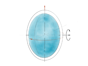
  $\boldsymbol {\varOmega }_{\boldsymbol {p}}=\hat {\boldsymbol {k}}_{\boldsymbol {p}}\varOmega _p$ fixed in the inertial frame of reference (see figure 1a). Here, $\hat {\boldsymbol {k}}_{\boldsymbol {s}}$ denotes the rotation vector and $\hat {\boldsymbol {k}}_{\boldsymbol {p}}$ the precession vector. For the description of the problem we choose a right-handed Cartesian coordinate system in which the $z$-axis is always aligned with the spin axis along $c$. Using $\varOmega _s^{-1}$ as the time scale and $R=(abc)^{1/3}$ as the length scale, the dimensionless Navier–Stokes equations in the frame of the container are
 $$\begin{gather} \frac{\partial \boldsymbol{u}}{\partial t} + 2(\hat{\boldsymbol{k}}_{\boldsymbol{s}} + Po \hat{\boldsymbol{k}}_{\boldsymbol{p}}) \times \boldsymbol{u} + \boldsymbol{u} \boldsymbol{\cdot} \boldsymbol{\nabla} \boldsymbol{u} ={-} \boldsymbol{\nabla} p - Po(\hat{\boldsymbol{k}}_{\boldsymbol{p}} \times \hat{\boldsymbol{k}}_{\boldsymbol{s}}) \times \boldsymbol{r} + E \boldsymbol{\Delta} \boldsymbol{u}, \end{gather}$$
 $$\begin{gather}\boldsymbol{\nabla} \boldsymbol{\cdot} \boldsymbol{u} = 0, \end{gather}$$
where  $\boldsymbol {u}$ is the flow velocity and $p$ is the reduced pressure including centrifugal forces. The two non-dimensional numbers in (2.1), are the Poincaré number $Po = \varOmega _p/\varOmega _s$, that measures the strength of the precession forcing and the classical Ekman number $E = \nu /\varOmega _s R^{2}$, with $\nu$ the kinematic viscosity.

Figure 1. (a) Sketch of the experimental device. (b) Close-up photography of the container and definition of the coordinate system. The  $x$-axis is pointing towards the reader.
Following Hough (Reference Hough1895), Sloudsky (Reference Sloudsky1895) and Poincaré (Reference Poincaré1910), let us search for a solution in the form of a uniform vorticity component written in the frame of the container as
 \begin{equation} \boldsymbol{U} = \boldsymbol{\omega} \times \boldsymbol{r} + \boldsymbol{\nabla} \psi, \end{equation}
where  $\boldsymbol {\omega } \times \boldsymbol {r}$ represents a rigid body rotation, with r the position vector $(x, y, z)$ and ω the fluid rotation vector ( $\boldsymbol{\omega}_x$, $\boldsymbol{\omega}_y$, $\boldsymbol{\omega}_z$) and $\boldsymbol {\nabla } \psi$ the irrotational stretching term necessary to enforce the non-penetrating boundary condition $\boldsymbol {u}\boldsymbol {\cdot }\hat {\boldsymbol {n}} = 0$ at the wall of the container. Using a set of coordinates fixed in the frame attached to the container with $\hat {\boldsymbol {x}}$ along $a$,
$a$,  $\hat {\boldsymbol {y}}$ along $b$ and $\hat {\boldsymbol {z}}$ along $c$, the velocity field (2.3) is expressed as
 $$\begin{gather} U_x = \omega_y \frac{2a^2}{a^2+c^2}z - \omega_z \frac{2a^2}{a^2+b^2}y, \end{gather}$$
 $$\begin{gather}U_y = \omega_z \frac{2b^2}{a^2+b^2}x - \omega_x \frac{2b^2}{c^2+b^2}z, \end{gather}$$
 $$\begin{gather}U_z = \omega_x \frac{2c^2}{b^2+c^2}y - \omega_y \frac{2c^2}{a^2+c^2}x. \end{gather}$$
Substituting this ansatz in (2.1), Noir & Cébron (Reference Noir and Cébron2013) derived the equations governing the evolution of the three components of the rotation vector  $\boldsymbol {\omega }$ in the frame of reference attached to the container, which we present here for a triaxial ellipsoid precessing at an angle of $90^\circ$:
 \begin{align} \frac{\partial \omega_x}{\partial t}&= \left[\frac{2a^{2}}{a^{2}+c^{2}}-\frac{2a^{2}}{a^{2}+b^{2}}\right]\omega_z\omega_y + Po \sin(t) \frac{2a^{2}}{a^{2}+b^{2}}\omega_z\nonumber\\ &\quad + \frac{2a^{2}}{a^{2}+c^{2}}\omega_y+ Po \sin(t)+\mathcal{L}\varGamma_x, \end{align}
 \begin{align} \frac{\partial \omega_y}{\partial t} &= \left[\frac{2b^{2}}{a^{2}+b^{2}}-\frac{2b^{2}}{b^{2}+c^{2}}\right]\omega_x\omega_z + Po \cos(t) \frac{2b^{2}}{a^{2}+b^{2}}\omega_z\nonumber\\ &\quad - \frac{2b^{2}}{b^{2}+c^{2}}\omega_x+ Po \cos(t)+\mathcal{L}\varGamma_y, \end{align}
 \begin{align} \frac{\partial \omega_z}{\partial t} &= \left[\frac{2c^{2}}{b^{2}+c^{2}}-\frac{2c^{2}}{a^{2}+c^{2}}\right]\omega_x\omega_y - Po \cos(t) \frac{2c^{2}}{a^{2}+c^{2}}\omega_y \nonumber\\ &\quad - Po \sin (t)\frac{2c^{2}}{b^{2}+c^{2}}\omega_x +\mathcal{L}\varGamma_z, \end{align}
where  $\boldsymbol {\varGamma }$ is the viscous torque and $\mathcal {L}$ is a matrix accounting for the geometry of the cavity
 \begin{equation} \mathcal{L}=\frac{15}{16\pi} \begin{bmatrix} \dfrac{b^2+c^2}{b^2c^2} & 0 & 0 \\ 0 & \dfrac{a^2+c^2}{a^2c^2} & 0 \\ 0 & 0 & \dfrac{b^2+a^2}{b^2a^2} \end{bmatrix} . \end{equation}
 Assuming a laminar Ekman boundary layer, Busse (Reference Busse1968), Noir et al. (Reference Noir, Cardin, Jault and Masson2003) and Noir & Cébron (Reference Noir and Cébron2013) derived expressions for the viscous torque in the asymptotic limit of small Ekman and Poincaré numbers. The viscous torque arises from the differential rotation between the fluid and the container,  $\boldsymbol {\delta \omega }$, which we decompose into an axial ( $\boldsymbol {\delta \omega }_{ax}$) and equatorial component ( $\boldsymbol {\delta \omega }_{eq}$) with respect to the fluid rotation axis. The two components are given by
 \begin{align} \boldsymbol{\delta \omega}_{ax}=\left(\frac{\boldsymbol{\varOmega}-\hat{\boldsymbol{k}}_s }{\varOmega^2} \boldsymbol{\cdot} \boldsymbol{\varOmega} \right)\boldsymbol{\varOmega}, \end{align}
 \begin{align} \boldsymbol{\delta \omega}_{eq}=\boldsymbol{\varOmega}-\hat{\boldsymbol{k}}_s - \boldsymbol{\delta \omega}_{ax}, \end{align}
where we have introduced
 \begin{equation} \boldsymbol{\varOmega}=\boldsymbol{\omega}+\hat{\boldsymbol{k}}_s, \end{equation}
the fluid rotation vector as seen from the frame of precession, i.e. the turntable.
Assuming that the viscous torque acting on the fluid prevents the growth of a spin-over mode from the equatorial differential rotation and the spin-up of the fluid from the axial differential rotation, Noir & Cébron (Reference Noir and Cébron2013) derived the following expression for the viscous term:
 \begin{equation} \mathcal{L}\boldsymbol{\varGamma}=\sqrt{E\varOmega}\left( \lambda_r \begin{bmatrix}\varOmega_x\\\varOmega_y\\\varOmega_z-1\end{bmatrix} + \frac{\lambda_i}{\varOmega}\begin{bmatrix}\varOmega_y\\-\varOmega_x\\0\end{bmatrix} +\varepsilon ( \lambda_{sup} -\lambda_{r} ) \begin{bmatrix}\varOmega_x\\\varOmega_y\\\varOmega_z\end{bmatrix} \right), \end{equation}
where  $\lambda _r$ and $\lambda _i$ are the real and imaginary parts of the viscous correction to the spin-over mode and $\lambda _{sup}$ represents a spatially integrated decay rate of the axial rotation. Furthermore, we have introduced
 \begin{equation} \varepsilon=\frac{\varOmega^2-\varOmega_z}{\varOmega^2}, \end{equation}
a measure of the no spin-up condition introduced by Noir et al. (Reference Noir, Cardin, Jault and Masson2003). We refer to expression (2.14) as the full damping.
In the limit  $\varepsilon <\omega /\varOmega$, when the axial torque is negligible in comparison with the equatorial one, we may neglect the last term in (2.14), to obtain
 \begin{equation} \mathcal{L}\boldsymbol{\varGamma}=\sqrt{E\varOmega}\left( \lambda_r \begin{bmatrix}\varOmega_x\\\varOmega_y\\\varOmega_z-1\end{bmatrix} + \frac{\lambda_i}{\varOmega}\begin{bmatrix}\varOmega_y\\-\varOmega_x\\0\end{bmatrix} \right), \end{equation}
which is equivalent to the expression of the viscous torque in a spheroid from Busse (Reference Busse1968) and Noir et al. (Reference Noir, Cardin, Jault and Masson2003). We refer to (2.16) as the reduced damping.
While the inviscid left-hand side of (2.7)–(2.9) is exact, all the assumptions are contained in the parameterization of the viscous effects, and it is thus important to make a few remarks regarding their range of validity: first, the approximation of the torque by the decay of spin-over and axial spin-up is only valid for a laminar boundary layer, and we shall later see that this assumption is satisfied in our experiments. Additionally, the parameters for the viscous correction of the spin-over mode  $\lambda _r$ and $\lambda _i$ can be calculated only when the fluid rotation axis is aligned with one of the principal axes of the ellipsoid (Vantieghem Reference Vantieghem2014). Finally, to the best of our knowledge, there is no analytical expression of $\lambda _{sup}$ in a non-axisymmetric ellipsoid and one has to rely on experimental estimates for this parameter. In conclusion, we note that, while the model will prove to be robust for small to moderate values of $Po$, we should keep in mind these limitations when discussing experiments with a large differential rotation between the fluid and the container or with a large tilt of the fluid rotation axis. In the remainder of this article, we will use $\lambda _r=-2.55$ and $\lambda _i=0.79$ as calculated from Vantieghem (Reference Vantieghem2014) for the geometry of our ellipsoid and for $\lambda _{sup}$ we use an experimentally determined value of $-2.50$, which is explained in further detail in Appendix A.
2.2. Numerical integration
In contrast to the spheroidal geometry, the governing equations for a non-axisymmetric ellipsoid are not in the form of an implicit equation and we must solve the system by time stepping the system of ordinary differential equations (ODEs) (2.7)–(2.9). To capture potential multiple solutions of the system, we randomly select  $300$ initial rotation vectors $\boldsymbol {\omega }$ by uniformly sampling the three variables $(\omega,\theta,\phi )$ in the range $([0,1],[0,2\pi ],[0,2\pi ])$ from which we construct the initial rotation vectors as $\omega _x = \omega \sin (\theta )\cos (\phi ),\omega _y = \omega \sin (\theta )\sin (\phi )$ and $\omega _z = \omega ^2 \cos (\theta ))$. Starting from the respective initial condition, we numerically integrate the (2.7)–(2.9) for 30 viscous spin-up times. Figure 2 represents the time averaged amplitude of the fluid rotation vector $\langle | \boldsymbol {\omega } | \rangle _t$ at the same conditions as our experiment. A more detailed discussion of the time evolution of the uniform vorticity in our numerical model can be found in Appendix B. In a range from $Po_c^1 = 0.075\pm 0.005$ to $Po_c^2 = 0.23\pm 0.005$, the system admits two solutions at each $Po$, as previously reported for axisymmetric spheroids (Cébron Reference Cébron2015; Nobili et al. Reference Nobili, Meunier, Favier and Le Bars2020).

Figure 2. Time averaged amplitude of the fluid rotation vector from the numerical integration of (2.7)–(2.9): two distinct branches of solution are identified and bi-stability (grey) is observed for  $0.075\pm 0.005< Po<0.23\pm 0.005$. The colours represent the number of randomly selected initial conditions converging to the respective solution. The values of $a$,
$a$,  $b$ and $c$ are the exact same ones as in the experiment.
3. Experimental set-up and flow measurements
3.1. Experimental set-up
The experimental set-up is sketched in figure 1(a). An ellipsoidal acrylic container of semi-major axes  $a = 0.125\ \text {m}$, $b= 0.104\ \text {m}$ and $c = 0.078\ \text {m}$ is rotating around $c$ using a servomotor (type: SGMGV-09DDA6F, produced by YASKAWA) and a belt driving system. The rotation rate $\varOmega _s$ is set to 1.57 rad s $^{-1}$. To create a precessional forcing, the rotating tank and the drive system are mounted on a turntable driven by another belt system connected to a second servomotor (type: SGMGH-30DCA61, produced by YASKAWA). The precession rate $\varOmega _p$ can be varied between 0.018 and 3.674 rad s $^{-1}$ in increments of 0.018 rad s $^{-1}$. The angle between $\boldsymbol {\varOmega }_{\boldsymbol {p}}$ and $\boldsymbol {\varOmega }_{\boldsymbol {s}}$, i.e. the precession angle, is fixed to $90^\circ$. The container is completely filled with water at room temperature with a kinematic viscosity $\nu =1\times 10^{-6}\ \text {m}^2\ \text {s}^{-1}$. The experimental values of the non-dimensional parameters introduced above are $6.3\times 10^{-5}$ for the Ekman number and the Poincaré number is varied between $0.035$ and $0.33$.
3.2. Flow measurements
We measure the flow inside the ellipsoid with ultrasonic Doppler velocimetry (UDV) from which we recover velocity profiles along selected chords in the fluid. To that end, the fluid is seeded with a mixture of 2AP1 Particles produced by Griltex, of sizes 50  $\mathrm {\mu }$m (60 % by weight) and 80 $\mathrm {\mu }$m (40 % by weight). The density of the tracer particles is $1.02$ g cm $^{-3}$. We use a DOP4010 system produced by Signal Processing SA,1073 Savigny, Switzerland, which allows us to simultaneously measure three velocity profiles at a sampling rate up to 12 Hz on each probe. Each profile consists of $\sim$500 individual sampling points along the chord with a spatial resolution of 0.5 mm.
The probe location has been carefully chosen to allow a direct measurement of the uniform vorticity component (2.4)–(2.6). The precise locations of the transducers are presented in table 1. To illustrate the concept of our determination of the fluid rotation  $\omega _x,\omega _y$ and $\omega _z$, let us consider the probe measuring $u_x$, i.e. probe 1 in figure 1(b), located at $y=0$ and $z=-0.47$ (in dimensionless units) and measuring in direction of $x$. In the direction of measurement, the uniform vorticity component $U_x$ is constant along the chord and takes the value $U_x=\omega _y (2a^2)/(a^2+c^2)(-0.47)$. Hence, we can use the velocity average along the chord $\langle u_x\rangle _x$, where $\langle \rangle _x$ denotes the spatial average along $x$, as a proxy for $\omega _y$. Placing two additional probes in the same fashion, we can reconstruct all three components of $\boldsymbol {\omega }$ as a function of time. In the rest of the paper, unless explicitly stated, all velocities are in dimensionless units, i.e. re-scaled by $\varOmega _s R$.
Table 1. Position of the UDV probes (centre of the front lens), measured velocity components ( $\boldsymbol {u}_{\boldsymbol {i}}$) and associated component of the fluid rotation vector ( $\boldsymbol {\omega }_{\boldsymbol {i}}$). All coordinates are non-dimensional.

Figure 3(a) illustrates a typical measurement of the velocity components  $u_x, u_y$ and $u_z$ and the corresponding time series of the deduced uniform vorticity at $Po=0.05$ (figure 3b). At leading order, the velocity is constant along the profile, in agreement with the uniform vorticity assumption. The uniform vorticity is dominated by the equatorial components $\omega _x$ and $\omega _y$, which are oscillating at $\varOmega _s$, while the axial component $\omega _z$ is characterized by a small, steady retrograde rotation and a oscillation at $2\varOmega _s$.

Figure 3. Typical velocity measurements in the experiment: (a) velocity profiles at  $Po = 0.05$. (b) Computing the spatial average along each profile allows us to reconstruct the three components of the uniform vorticity $\boldsymbol {\omega }$ as a function of time. The error bars display the standard deviation of the spatial average. The Ekman number is $6.30\times 10^{-5}$ and $x$,
$x$,  $y$ and $z$ in (a) are made dimensionless by $R$ and the time in (b) is made dimensionless by $\varOmega _s$.
3.3. Experimental protocol
We apply the following experimental protocol: the container is set into rotation at  $\varOmega _s$ and we wait until the fluid co-rotates with the container, which is indicated by a vanishing velocity on all UDV channels. Subsequently, we start the motion of the turntable at $\varOmega _p$ and wait until a statistically steady state is reached. We then start our measurements collecting 3000 samples on each channel at a sampling frequency of 12 Hz. Finally, we change the precession rate to the next value of $\varOmega _p$ and wait again until the fluid motion at the increased precession rate is in a steady state. We perform two sets of experiments: in the first one we subsequently increase $Po$ from $Po=0.035$ to $Po=0.33$, in the second set of experiments we start from $Po=0.33$ and decrease the precession rate down to $Po=0.035$.
4. The uniform vorticity
4.1. Overview of the results
We start with a discussion of the uniform vorticity component and define four important quantities that characterize the rotation of the fluid: first, the time averaged total rotation of the fluid  $\langle \varOmega \rangle _t$, second, the time averaged differential rotation between the fluid and the container, $\langle \delta \omega \rangle _t$, third, the time average rotation of the fluid along the spin axis $\langle \varOmega _z\rangle _t$ and, finally, the time averaged tilt angle of the fluid rotation axis with respect to the container axis, $\langle \theta \rangle _t$. These quantities are defined in the frame of precession, i.e. viewed from the turntable, and can be obtained from our measurements of $\omega _x$, $\omega _y$ and $\omega _z$ as follows:
 $$\begin{gather} \langle \varOmega\rangle _t=\langle \sqrt{\omega_x^2+\omega_y^2+(\omega_z+1)^2}\rangle _t , \end{gather}$$
 $$\begin{gather}\langle \delta \omega \rangle _t=\langle \sqrt{\omega_x^2+\omega_y^2+\omega_z^2}\rangle _t , \end{gather}$$
 $$\begin{gather}\langle \varOmega_z\rangle _t=\langle \omega_z+1\rangle _t, \end{gather}$$
 $$\begin{gather}\langle \theta\rangle _t= \left\langle \arccos \frac{\varOmega_z}{\varOmega}\right\rangle _t, \end{gather}$$
where  $\langle \rangle _t$ denotes the average in time. The experimental data for the four quantities as a function of $Po$ are presented in figure 4, together with the prediction from the model (2.7)–(2.9), using the full damping (blue curve) and the reduced damping (red curve). As we have seen above, the model predicts two distinct branches of solutions in the range $Po_c^1=0.075\pm 0.005< P_o< Po_c^2=0.23\pm 0.005$, indicated by the grey area. We call branch 1 the solutions characterized by a large total fluid rotation, a small differential rotation, a large axial rotation and a moderate tilt angle. In contrast, the solutions of branch 2 have a small total fluid rotation, a large differential rotation of ${O}(1)$, a vanishing axial rotation and a large tilt angle.

Figure 4. Fluid rotation viewed from the precession frame: (a) total fluid rotation. (b) Differential rotation  $\langle \delta \omega \rangle _t$ between the fluid and the container. (c) Axial component of rotation of the fluid. (d) Angle between the fluid and container axis of rotation. The points represent the experimental data, circles when increasing $Po$, triangles when deceasing $Po$. The solid and dashed lines represent the model branches 1 and 2, respectively, for the full damping (blue) and the reduced damping (red). The shaded area represents the range of $Po$ for which the model accepts two solutions. The two bounds of this region are $Po_c^1=0.075\pm 0.005$ and $Po_c^2=0.23\pm 0.005$. The arrows materialize the experimental transition from branch 1 to branch 2 and vice versa. All experiments are performed at $E=6.3\times 10^{-5}$ and the parameters for the damping in the model are $\lambda _r=-2.55$, $\lambda _i=0.79$ and $\lambda _{sup}=-2.50$. The error bars are representative of the standard deviation of the displayed quantities over the entire time series.
Experimentally, as we start from the smallest values in  $Po\approx 0.03$ and subsequently increase $Po$ between the individual experiments, we follow the solutions of branch 1 until a critical value $Po_{exp}^2=0.18\pm 0.006$ is reached. At this point, the uniform vorticity component in the experiment transits to branch 2, where it remains for all larger $Po$ values. In contrast, when decreasing $Po$ after starting from large values $Po\approx 0.33$, the experimental data follow branch 2 down to $Po_{exp}^1=0.11\pm 0.006$, from where they transit to branch 1. Outside of the hysteresis region ranging from $Po_{exp}^1$ to $Po_{exp}^2$, the measured quantities for increasing and decreasing $Po$ overlap almost perfectly. Comparing the model with the experimental data, we observe a very good agreement in branch 1 for all four quantities. However, in branch 2 the model systematically underestimates the differential rotation and the tilt of the fluid rotation axis. Moreover, the model predicts a small positive axial rotation whereas we observe negative values in the experiment. Nevertheless, it is fair to say that the model still captures the fundamental properties of this second branch correctly.
We notice that  $Po_{exp}^{1}$ and $Po_{exp}^{2}$ in the experiment do not match exactly the boundaries of the hysteresis domain of the model. For both, increasing and decreasing $Po$, the experimental data transit to the other branch before the end of the hysteresis range in the model. As we shall see later, both transitions occur in a range of $Po$ where fully developed instabilities are observed, with amplitudes comparable to that of the underlying uniform vorticity flow. In such conditions it is likely that finite amplitude perturbations may trigger early transitions, in comparison with the uniform vorticity model, which is free of any perturbations or instabilities by construction. Alternatively, since the fluid rotation is no longer close to the container axis, it may be argued that the asymptotic values of the damping coefficients $\lambda _r,\lambda _i$ and $\lambda _{sup}$ are not representative of the boundary layer dynamics in this range of $Po$. In Appendix C we consider finite variations of the three damping coefficients, demonstrating that no set of values ( $\lambda _r,\lambda _i,\lambda _{sup}$) can consistently explain our observations. Using different values of $\lambda _r,\lambda _i$ and $\lambda _{sup}$ for each $Po$ may seem somewhat more physical and might even yield a better agreement between experimental data and model, however, there is a high risk of over-fitting the data, especially in the absence of an underlying physical model. We believe it is more appropriate to use the model with the asymptotic values and keep in mind the limitations of its validity range.
4.2. Spin-over and spin-up damping contribution
Integrating the system of ODEs with the full and the reduced damping yields almost identical solutions, as indicated by the similarity between the blue and red curves in figure 4. Both damping models fit equally well the data at the smallest  $Po$ in branch 1 while showing a less good agreement at larger $Po$, which suggest that the viscous torque is dominated by the spin-over component over the entire range of explored $Po$. From the expression of the viscous term (2.14), we calculate the time averaged amplitude of the spin-over contributions $\langle | \mathcal {L}\varGamma _{so} |\rangle _t$ and spin-up contribution $\langle | \mathcal {L}\varGamma _{sup} |\rangle _t$ as
 $$\begin{gather} \langle|\mathcal{L}\boldsymbol{\varGamma}_{sup} |\rangle _t= \langle |\varepsilon\sqrt{E\varOmega} \lambda_{sup} \boldsymbol{\varOmega} |\rangle _t, \end{gather}$$
 $$\begin{gather}\langle |\mathcal{L}\boldsymbol{\varGamma}_{so} |\rangle _t =\langle | \mathcal{L}\boldsymbol{\varGamma} - \mathcal{L}\boldsymbol{\varGamma}_{sup}|\rangle _t. \end{gather}$$
The results for branch 1 and branch 2 solutions are depicted in figure 5. Over the entire range of investigated  $Po$ values, both the model and the experiment are dominated by the spin-over viscous term, which explains the close similarity between the full and reduced model. In branch 1, the damping from the model is in excellent agreement with the experimental data, with a spin-over contribution one order of magnitude larger than the spin-up. In branch 2, the model still captures the dominance of the spin-over contribution correctly but the actual amplitude of both torques is larger in the experiment, which may be a signature of nonlinear contributions which are not accounted for in the model.

Figure 5. Comparison of the spin-over (red) and spin-up (green) damping term in the experiment and in the model. (a) Branch 1 solutions (solid line). (b) Branch 2 solutions (dashed line).
These findings suggest that the so-called no spin-up condition in a spheroid as derived by Busse (Reference Busse1968) and Noir et al. (Reference Noir, Cardin, Jault and Masson2003), i.e.  $(\varOmega ^2-\varOmega _z)/\varOmega ^2=0$, may also hold at small $Po$ in an non-axisymmetric ellipsoid. Figure 6 shows $\langle |\varepsilon |\rangle _t= \langle |(\varOmega ^2-\varOmega _z)/\varOmega ^2 |\rangle _t$ as a function of $Po$ for the solutions of branches 1 and 2 from the model and the experiment, confirming that the no spin-up condition is a reasonable assumption at small $Po$ in branch 1. In branch 2, this condition is clearly violated, as the experimental data and the model display values $>1$.
$>1$.

Figure 6. Measure of the no spin-up condition  $\langle |\varepsilon |\rangle _t= \langle |(\varOmega ^2-\varOmega _z)/\varOmega ^2 |\rangle _t$ in the experiment. The error bars are representative of the standard deviation of the displayed quantities over the entire time series.
5. Non-uniform vorticity flow
5.1. Kinetic energy in the uniform and non-uniform vorticity flow
By construction, the semi-analytical model only accounts for the uniform vorticity component of the flow, which may not be dominant at large  $Po$. Considering the flow in the frame of precession, the velocity can be decomposed into its uniform vorticity component, hereafter referred to as the base flow Ub and the non-uniform vorticity components $\boldsymbol{u}_{non}$:
 \begin{equation} \boldsymbol{u}=\boldsymbol{U}_b +\boldsymbol{u}_{non}, \end{equation}
with
 \begin{equation} \boldsymbol{U}_b=\boldsymbol{\varOmega}\times \boldsymbol{r}+\boldsymbol{\nabla}\psi. \end{equation}
We define the associated mean kinetic energy as
 $$\begin{gather} E_b=\frac{1}{V}\int \frac{\boldsymbol{U}_b^2}{2} \,\textrm{d}v, \end{gather}$$
 $$\begin{gather}E_{non}=\frac{1}{V}\int \frac{(\boldsymbol{u}-\boldsymbol{U}_b)^2}{2} \,\textrm{d}v. \end{gather}$$
 In figure 7(a) we present the time averaged ratio  $\langle E_{non}/E_{b}\rangle _t$ when increasing and decreasing $Po$ in branches 1 and 2. The dynamics evolves from a largely dominant uniform vorticity flow in branch 1 to a state of almost equal kinetic energy in the uniform and non-uniform vorticity flow. Comparing the individual energies $\langle E_{b}\rangle _t$ and $\langle E_{non}\rangle _t$ we observe two distinct behaviours: the base flow amplitude hardly evolves over the entire branch 1, but abruptly drops by a factor of 10 across the transition to branch 2 at $Po_{exp}^2$ (figure 7b). In contrast, $\langle E_{non}\rangle _t$ increases continuously by almost two orders of magnitude in branch 1, reaching a saturation value that also holds in branch 2 with a much smaller jump at the branch transition (figure 7c). The increasing amplitude of the fluctuating velocity component $u_{non}$ at larger forcing amplitude is also reflected in the more complex flow regime, as can be anticipated from movies of qualitative flow visualization using rheoscopic fluid (Borrero-Echeverry, Crowley & Riddick Reference Borrero-Echeverry, Crowley and Riddick2018), which we provide as supplementary movies are available at https://doi.org/10.1017/jfm.2021.932.

Figure 7. (a) Time averaged ratio of the non-uniform vorticity flow and the base flow mean kinetic energy  $E_{non}/E_{b}$ as a function of $Po$; (b) uniform vorticity base flow mean kinetic energy $E_{b}$ as a function of $Po$; (c) non-uniform vorticity flow mean kinetic energy $E_{non}$ as a function of $Po$. The colour scheme characterizes the branch of solution, the two symbols represent the increasing/decreasing $Po$ experiments. The error bars are representative of the standard deviation of the displayed quantities over the entire time series. The unit of energy is $(\varOmega _sR)^2$.
5.2. Instabilities
After characterizing its amplitude, we now aim at shedding light on the dynamical nature of the non-uniform vorticity flow. Three instability mechanisms have been identified in precessing fluid cavities: parametric resonances (Kerswell Reference Kerswell1993; Goto et al. Reference Goto, Ishii, Kida and Nishioka2007; Lin et al. Reference Lin, Marti and Noir2015), viscous boundary layer instabilities (Tilgner & Busse Reference Tilgner and Busse2001; Cébron et al. Reference Cébron, Laguerre, Noir and Schaeffer2019; Nobili et al. Reference Nobili, Meunier, Favier and Le Bars2020; Buffett Reference Buffett2021) and, more recently, experiments and numerical simulations suggest that centrifugal instabilities may occur in precessing cylinders leading to space filling turbulence (Giesecke et al. Reference Giesecke, Vogt, Gundrum and Stefani2018, Reference Giesecke, Vogt, Gundrum and Stefani2019). Our spatially limited UDV measurements may not allow us to completely disentangle these mechanisms, for example we cannot get access to the radial profile of the angular momentum that plays a crucial role in the identification of the centrifugal instability reported by Giesecke et al. (Reference Giesecke, Vogt, Gundrum and Stefani2018). Nevertheless, we can still gain insights into the evolution of instabilities from the spectral content of  $\boldsymbol {u}_{non}$. To that end, we calculate the discrete Fourier transform (DFT) in time of $\boldsymbol {u}_{non}$, at all positions along the three velocity profiles. We then take the spatial average along each chord, to obtain the space averaged spectral content of $u_{non,x}, u_{non,y}$ and $u_{non,z}$. Finally, we stack all three DFT components and the resulting spectra are presented in figure 8a) for increasing $Po$ and figure 8b) for decreasing $Po$. At very small $Po\leq 0.11$, we observe only frequencies corresponding to the forcing at dimensionless frequency $\varpi /\varOmega _s=1$ and $\varpi /\varOmega _s=2$. Following branch 1 for $Po\geq 0.12$ up to the transition at $Po=0.18$ (figure 8a) we distinguish individual peaks which satisfy the typical parametric resonant conditions $\varpi _1 \pm \varpi _2=\varpi$, with $\varpi = \varOmega _s$ or $\varpi =2\varOmega _s$ near onset (Kerswell Reference Kerswell1993; Lin et al. Reference Lin, Marti and Noir2015), where the instability saturates via viscous and/or detuning effects. After the transition to branch 2, the spectra are again characterized by dominating peaks $\varpi /\varOmega _s=1$ and $\varpi /\varOmega _s=2$, but this time significant energy is widely spread over all frequencies. This observation is characteristic for all experiments of branch 2, also for the experiments at decreasing $Po$ depicted in figure 8b)

Figure 8. Stacked DFT in time of  $u_{non}$. Each spectrum is normalized by the respective Po. (a) DFT for increasing Po; (b) DFT decreasing Po. Blue and orange colours mark branch 1 and branch 2, respectively.
We observe typical growth and collapses of the instability as illustrated in figure 9 for the smallest  $Po$ of branch 2, i.e. at $Po = 0.13$, where we observe a decay of the base flow during the growth of the instability until a state is reached, where base flow and instability have almost the same kinetic energy. At that point, the instability collapses and allows the base flow to recover its initial amplitude. These cycles of growth and collapse are typical of weakly super critical parametric instabilities (Malkus Reference Malkus1989; Eloy, Le Gal & Le Dizes Reference Eloy, Le Gal and Le Dizes2003; Herreman et al. Reference Herreman, Cébron, Le Dizès and Le Gal2010) and somewhat reminiscent of the intermittent solution as predicted by the amplitude equations for the weakly nonlinear instability in a precessing cylinder reported by Lagrange et al. (Reference Lagrange, Meunier, Nadal and Eloy2011). At larger $Po$, the temporal dynamics of the flow becomes more and more complex, with shorter period of growth and collapse and eventually indistinguishable cycles.

Figure 9. Time series of  $E_{non}$ and $E_b$ for the lowest $Po=0.129$ of branch 2. The background grey curves correspond to the unfiltered data, the coloured curves represent a running averaging of the energies with a window of 1.5 rotations.
Concerning boundary layer instabilities, it is suggested that instabilities of a steady Ekman boundary layer should occur at  $Re_{bl}>55$ and a transition to turbulence at $Re_{bl}>150$ (Caldwell & Van Atta Reference Caldwell and Van Atta1970; Sous et al. Reference Sous, Sommeria and Boyer2013), where $Re_{bl}$ is the Reynolds number based on the thickness of the Ekman layer. However, the recent numerical study of Buffett (Reference Buffett2021) suggests that, for oscillating flows, such as the ones driven by precession, the Ekman boundary layer would only become turbulent at $Re_{bl}>500$. We define the boundary layer Reynolds number based on the amplitude of the differential rotation between the wall and the fluid $\delta \omega$ as $Re_{bl}=\delta \omega E_f^{-1/2}$, where $E_f$ is the effective Ekman number based on the fluid rotation $\varOmega$. With our notation it follows that
 \begin{equation} Re_{bl}=\langle \delta \omega \rangle _t (E/\langle \varOmega\rangle _t)^{{-}1/2}. \end{equation}
As shown in figure 10, Ekman boundary layer instabilities may occur in branch 2, yet never reach the onset condition for turbulence. Consequently, the instabilities reported above starting at  $Po\sim 0.117$, could not be underlined by a boundary layer mechanism.

Figure 10. Boundary layer Reynolds number  $Re_{bl}=\delta \omega (E\varOmega )^{-1/2}$ as a function of $Po$ in branches 1 and 2. The dashed black line represents the onset range $Re_{bl}>55$ for the initial boundary layer instability.
To conclude this section, we shall briefly discuss the evolution of the Rossby number based on the fluctuating velocity component  $\boldsymbol {u_{non}}$ and the fluid rotation
 \begin{equation} Ro=\frac{\langle (2E_{non})^{1/2}\rangle _t}{\langle \varOmega\rangle _t R}. \end{equation}
In figure 11 we display  $Ro$ as a function of $Po$ for our experimental data. In branch 1, $Ro$ increases from $\sim$0.01 to $\sim$0.06, in agreement with the increasingly nonlinear dynamics observed from the frequency spectra, yet remaining less than unity. In contrast, branch 2 is characterized by a Rossby number greater than one, giving rise to a strongly nonlinear dynamics. Given the reported values of $Ro>0.5$ it is difficult to apprehend this regime, as it may no longer follow the classical rotating nor non-rotating dynamics. Further investigations will be necessary to fully comprehend this regime, in particular the emergence of a regime where $E_{b}$ and $E_{non}$ are of the same order is of great interest for dynamo experiments and industrial applications.

Figure 11. Effective Rossby number based on the fluctuating velocity component  $u_{non}$ and the total rotation of the fluid.
6. Conclusions
We have experimentally investigated the flows in a triaxial ellipsoid subject to precession at an angle of  $90^\circ$. We first focused on the base flow of uniform vorticity and, by exploiting symmetry properties of this flow, we measure the three components of the uniform vorticity flow using UDV. In agreement with a semi-analytical model for the evolution of the uniform vorticity proposed by Noir & Cébron (Reference Noir and Cébron2013), we observe two distinct branches of solutions: branch 1 is typically observed at small to moderate forcing ( $Po<0.18$) and is characterized by a large amplitude of the total fluid rotation ( $\sim$1 in dimensionless units), as well as a small angle between the fluid rotation and the rotation axis of the container. In contrast, branch 2 is characterized by a much smaller total rotation of the fluid and a large tilt of the fluid rotation axis, which tends to align with the axis of precession. Furthermore, we find a hysteresis cycle of the uniform vorticity component as a function of $Po$, from both the model and the experimental data. A remarkable agreement between the uniform vorticity model and experimental data is observed in branch 1, especially at small values of $Po$. This might justify the application of the model in the context of planetary core and subsurface ocean dynamics, which are typically characterized by a small amplitude of the forcing.
Although the model still captures the fundamental features of branch 2, the agreement with experimental data is less good. This is to be expected as the semi-analytical model is only valid at small  $Po$, yet the predictions remain in good enough qualitative agreement with the observations to capture the first-order dynamics of the system.
It is of great interest for both planetary science and industrial applications to characterize different instability mechanisms in precessing flows, which could lead to space filling turbulence. Our results suggest that a parametric instability mechanism occurs early in branch 1 and evolves towards a complex saturated state in branch 2 with a kinetic energy comparable to that of the underlying base flow. It should be emphasized that our observation of a hysteresis in the amplitude of the uniform vorticity base flow is not necessarily related to that of turbulence (as reported by e.g. Malkus Reference Malkus1968; Herault et al. Reference Herault, Gundrum, Giesecke and Stefani2015; Horimoto et al. Reference Horimoto, Simonet-Davin, Katayama and Goto2018; Komoda & Goto Reference Komoda and Goto2019), while the opposite is likely true. In fact, one could imagine a scenario where branch 2 of the base flow is not necessarily unstable. Nevertheless the observation of the fluctuating velocities being of the same order as the base flow in branch 2, as well as the qualitative flow visualization (see supplementary movies), point towards the first scenario in our experiment. Of course it would be quite valuable to draw a conclusive picture of the transition to turbulence in various container shapes, (i.e. in cylinder, spheres, spheroids and ellipsoids) but this is beyond the focus of the present article.
The observation of a state with same order of kinetic energy in the base flow and fluctuating velocity component provides a reasonable estimate for the typical  $u_{non}$ in industrial applications operating in similar range of parameters, i.e. $E\gtrsim 10^{-6}$ and $Po\sim 1$. In planetary settings, i.e. $E\sim 10^{-14}$, it has been suggested that the saturation mechanism of the instabilities might be fundamentally different, i.e. inertial wave turbulence instead of geostrophic turbulence (Le Reun et al. Reference Le Reun, Favier and Le Bars2019). Whether a state of quasi-equal kinetic energy holds in planetary cores or subsurface oceans remains an open question. Further investigations at much lower Ekman numbers will be necessary, such as the one accessible in the upcoming Dresdyn experiment (Stefani et al. Reference Stefani, Albrecht, Gerbeth, Giesecke, Gundrum, Herault, Nore and Steglich2015).
Supplementary movies
Supplementary movies are available at https://doi.org/10.1017/jfm.2021.932.
Acknowledgements
The authors acknowledge insightful discussions with D. Cebron, M. Le Bars and P. Meunier and the assistance of A. Leuthold in the construction of the experimental device. We thank three reviewers for constructive comments and suggestions.
Funding
This research was supported by Swiss National Science Foundation grant 200021_140708, Swiss National Science Foundation grant no. 200021_165641, Swiss National Science Foundation grant no. 200021_185088 and ETH Research Grant ETH-26 15-1.
Declaration of interests
The authors report no conflict of interest.
Appendix A. Spin-up in a triaxial ellipsoid
To the best of our knowledge, no formulation exists for the decay rate of the axial rotation in a non-axisymmetric container, and thus an estimate for  $\lambda _{sup}$ has to be determined experimentally. To that end, we conducted a number of axial spin-up experiments to obtain estimates of $\lambda _{sup}$ under the following experimental protocol: we set the container into constant rotation at $\varOmega _0$ around the $c$-axis and then increase the rotation rate by a small amount $\delta \varOmega$, which creates an initial differential rotation of the fluid with respect to the container. In order to keep the spin-up in the laminar regime, we choose $\delta \varOmega$ in such a way that the Rossby number $\delta \varOmega /\varOmega _0$ remains small. Following Greenspan & Howard (Reference Greenspan and Howard1963), the differential motion decays exponentially with time as
 \begin{equation} \boldsymbol{\delta\omega}_{ax}(t,\boldsymbol{r}) = \boldsymbol{\delta\omega}_{ax}(0)[1-\exp(\lambda_{sup}(\boldsymbol{r}) \sqrt{E} t)], \end{equation}
with the decay factor  ${\lambda _{sup}(\boldsymbol {r})}$. In general, $\lambda _{sup}$ locally depends on the height of the fluid column in the direction of the rotation axis and is thus a function of space. However, for our damping model we need to obtain a spatially averaged value of the decay factor acting on the axial components of the uniform vorticity and we thus fit the time series to the same quantity, which is $\langle \boldsymbol {\delta \omega }_{ax}\rangle _s$, where $\langle \,\rangle _s$ denotes the spatial average. In figure 12, we display inverted values of $\lambda _{sup}$ as a function of the Rossby number in the axial spin-up experiments. All experiments are recorded at Ekman numbers in the range of $1.5\times 10^{-5}$ to $6.3\times 10^{-5}$, comparable to the values of $E$ in our precession experiments. We observe considerable scatter around a mean value of $\lambda _{sup} \sim -1.89$ (dashed red line), but nevertheless our spin-up experiments give a maximum amplitude of $\lambda _{sup} > -2.5$, which allows us to estimate the contribution of the spin-up to the damping in (2.14).

Figure 12. Inverted values for the spatially averaged decay rate of the axial spin-up in a triaxial ellipsoid. Experiments were conducted at various  $Ro$ between $0.05$ and $0.2$. Range of Ekman numbers: $1.5\times 10^{-5}$ to $6.3\times 10^{-5}$.
Appendix B. Time evolution of the uniform vorticity model
In figure 13(a,b) we display the time evolution of the uniform vorticity as predicted from the numerical integration of (2.7)–(2.9)) computed for  $Po = 0.05$ and $Po=0.25$ representing typical solutions of branch 1 and branch 2, respectively. For both $Po$ we start from the randomly selected initial conditions $[\omega _x(0),\omega _y(0),\omega _z(0)]=[-0.166, -0.002, -0.213]$ and integrate the equations for an equivalent of 10 Ekman time scales. We display a time series, equivalent to six rotation times in steady state. To allow a comparison between model and experimental data, we additionally display the corresponding experimental data in light colours. Note that we artificially shifted the start of the experimental time series to be in phase with the numerical data.

Figure 13. Time evolution of the uniform vorticity model at  $Po=0.05$ (a,b) and at $Po=0.25$ (c,d) in branch 1 and branch 2, respectively. The solid line represents the solution as calculated with our model and the light colours show the experimental data at the exact same conditions for comparison. In (b) and (d), we display the spectral content of the amplitude of the uniform vorticity $|\boldsymbol{\omega} |$. Again, the light colours represent the experimental data for comparison.
In agreement with the experimental data we observe that the two equatorial components of the uniform vorticity  $\omega _x$ and $\omega _y$ show time harmonic oscillations at dimensionless frequency $\varpi /\varOmega =1$. For the axial component $\omega _z$ the model also predicts a time harmonic solution at dimensionless frequency $\varpi /\varOmega =2$, with a constant offset, which is in good agreement with the experimental data. However, the amplitude of the time harmonic oscillations in the axial component are underestimated in the model in comparison with the experimental data. In contrast to the experimental data there is no fundamental difference observed between branch 1 and branch 2 in the model. As expected, there is less of an agreement between model and data in branch 2, because our model cannot capture the increasingly nonlinear dynamics in this branch.)
Appendix C. Varying the damping coefficient of the semi-analytical model
The calculation of ( $\lambda _r,\lambda _r,\lambda _{sup}$) involves integrals over the fluid domain, which depend on $\theta$, the tilt of the fluid rotation axis with respect to the figure axis of the cavity. In our experiment $\theta$ varies from 0 to more than $90^{\circ }$, thus it could be argued that the asymptotic values used to integrate the model are not representative over the entire range of explored $Po$. In figure 14, we compare the experimental measurements with the semi-analytical models obtained by varying the damping parameters around their asymptotic values at $\theta \sim 0\ (Po\ll 1)$. We observe a high sensitivity of the model to both $\lambda _r$ and $\lambda _{sup}$, while $\lambda _i$ has limited effect on the solutions in branch 1. Increasing $\lambda _{sup}$ to large values could explain the early transition of branch 1 (figure 4a), however, the associated value of $\varepsilon$ for these solutions are already order ${O}(1)$ in branch 1, which is in contradiction to our observations (figure 6). Furthermore, it has no influence on transition from branch 2 to branch 1. Decreasing $\lambda _r$ merely improves the transition from branch 1 (figure 4) while making the branch 2 to branch 1 solution worse. Increasing $\lambda _r$ to large values improves the second transition but delays the first transition. It seems difficult to reconcile our observations by somewhat artificially fitting the damping parameters. While it may seem more physical to use different values of the damping as $\theta$ increases, no analytical models exist for an arbitrary orientation yet.

Figure 14. Comparison of the experimental total fluid rotation varying the damping parameters of the model. (a) Effect of  $\lambda _{sup}$, $\lambda _r=-2.55$ and $\lambda _i=0.79$. (b) Effect of $\lambda _i$, $\lambda _r=-2.55$ and $\lambda _{sup}=-2.5$. (c) Effect of $\lambda _r$, $\lambda _i=0.79$ and $\lambda _{sup}=-2.5$. The experimental data are the same as in figure 4(a). The solid lines represent the solution of branch 1, the dashed lines of branch 2.


 Open access