


1. Introduction
Many microfluidics devices have been developed to miniaturize cell culture and better mimic in vivo environments (Huh et al. Reference Huh, Matthews, Mammoto, Montoya-Zavala, Hsin and Ingber2010). Conventional devices are often made of solid plastics and standard equations for solid conduits can be applied to describe flow within them (Stone, Stroock & Ajdari Reference Stone, Stroock and Ajdari2004; Zhou & Papautsky Reference Zhou and Papautsky2013). When cells are cultured behind solid walls, gas bubbles often cause failures; additionally, solid boundaries prevent direct access to cell cultures that is often a fundamental request of bio-scientists. Consequently, an increasing number of open microfluidic technologies are being developed where some solid boundaries are replaced by liquid interfaces (Feng et al. Reference Feng, Mao, Dou, Li, Li and Lin2019; Dunne et al. Reference Dunne2020). When the Bond number is much less than 1, typically with volumes of one microliter or smaller, fluid behaviour is governed by interfacial forces as the effects of gravity and inertial forces become negligible. Then, an interface between two immiscible fluids can act as a confining wall just as an air/water interface confines rain drops on a windowpane; hence, we use the term fluid–wall as a synonym for liquid–liquid interfaces. Microfluidic circuits bounded by such interfaces can be manually/directly accessed simply by piercing through the self-healing liquid walls (Soitu et al. Reference Soitu, Feuerborn, Deroy, Castrejón-Pita, Cook and Walsh2019), and they will never fail due to trapped air bubbles (as they spontaneously rise to the surface). Moreover, circuits can be fabricated in standard Petri dishes, thus using materials well known to biologists (Berthier, Young & Beebe Reference Berthier, Young and Beebe2012). However, flows can no longer be predicted using equations derived for conduits with solid and rigid walls (Towell & Rothfeld Reference Towell and Rothfeld1966; Qian et al. Reference Qian, Joo, Jiang and Cheney2009; Christov et al. Reference Christov, Cognet, Shidhore and Stone2018; Raj, Suthanthiraraj & Sen Reference Raj, Suthanthiraraj and Sen2018; Martínez-Calvo et al. Reference Martínez-Calvo, Sevilla, Peng and Stone2019) as the fluid interfaces morph according to pressure. Recently, an innovative open technology known as ‘fluid-walled microfluidics’ has been developed that is proving especially useful for bio-scientists (Walsh et al. Reference Walsh, Feuerborn, Wheeler, Tan, Durham, Foster and Cook2017; Vallone et al. Reference Vallone, Telugu, Fischer, Miller, Schommer, Diecke and Stachelscheid2020). Cell environments are created in conventional Petri dishes by reshaping a thin layer of cell-culture medium overlaid by an immiscible liquid (often the biocompatible fluorocarbon, FC40). Reshaping is achieved by jetting more FC40 through a nozzle held by a three-way traverse that moves over the dish as it ’draws’ the desired pattern (figure 1a) (Soitu et al. Reference Soitu, Stovall-Kurtz, Deroy, Castrejón-Pita, Cook and Walsh2020). The FC40 jet sweeps medium away from the substrate, and leaves the overlay tightly pinned to the dish. These pinned walls confine the resulting aqueous circuit, isolating it from its surroundings (figure 1b). Such circuits have been used to perfuse cultured cells (Soitu et al. Reference Soitu, Stovall-Kurtz, Deroy, Castrejón-Pita, Cook and Walsh2020) and to perform chemotactic assays (Deroy et al. Reference Deroy, Rumianek, Wheeler, Nebuloni, Cook, Greaves and Walsh2022); however, flows were maintained using complex experimental set-ups and external pumps. Therefore, there is the need to develop automatic (‘passive’) pumping systems that do not rely on external active pumps. Walker & Beebe (Reference Walker and Beebe2002) proposed a passive pumping system that exploits Laplace pressure to drive flow from a source drop to a sink through a plastic rectangular conduit. A water drop was simply pipetted over an inlet, and the surface tension between water and the surrounding air generated a pressure across the interface (Laplace pressure) that pushed the aqueous phase through the conduit. Here, we use a similar pumping system that relies on Laplace pressure generated across the interface between the patterned medium and the immiscible overlay. Additionally, we propose a closed semi-analytical solution able to predict the flow rate over time while a source drop empties its volume through a fluid-walled conduit of known footprint geometry (as liquid interfaces above it morph), and we validate the quality of the predictive solutions via experiments.

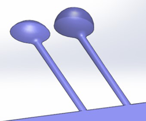
Figure 1. Circuit fabrication. (a) A three-dimensional and side view schematic of the fabrication process. (b) Example circuit printed in a Petri dish overlaid by clear FC40; close-up top view of the circuit.
2. Problem formulation
We will consider a simple circuit (figure 2a-i,ii) that exploits Laplace pressure to drive flow from a drop (the source), through a straight conduit into the rest of the dish (which acts as a sink). The aqueous phase throughout the circuit is bounded by the polystyrene substrate and fluid walls (i.e. an interface between two immiscible liquids). Flows driven by Laplace pressure through conduits entirely bounded by solid walls have been widely studied (Walker & Beebe Reference Walker and Beebe2002; Berthier & Beebe Reference Berthier and Beebe2007; Chen, Eckstein & Lindner Reference Chen, Eckstein and Lindner2009). Major determinants of flow include the pressure of the source drop and conduit geometry, with flows declining as the source drop empties. Whilst these determinants apply to our case, the fluid nature of walls introduces additional complexities. For example, the conduit cross-section inevitably morphs as pressure falls from inlet to outlet (figure 2a-iii). Recently, a simple power law has been proposed to describe height variation of a straight fluid-walled conduit when a constant flow rate is actively perfused through it (Deroy et al. Reference Deroy, Stovall-Kurtz, Nebuloni, Soitu, Cook and Walsh2021); it relates cross-sectional conduit height to the decrease in pressure down the length of the conduit. However, in our case, inlet pressure constantly varies as the source drop empties. Calver et al. (Reference Calver, Gaffney, Walsh, Durham and Oliver2020) presented an asymptotic analysis of this problem approximated using thin-film equations, but their solution lacks experimental validation and our approach simplifies the solution significantly. Considering the micrometric scale of our system, we assume interfacial forces dominate and pressure differences at all points in the system are exclusively defined by the Young–Laplace equation,  $\Delta P=\gamma (1/R_1 +1/R_2)$, where $\Delta P$ is the pressure difference across the interface, $\gamma$ is the interfacial tension of the pair of fluids, and $R_1$ and $R_2$ are two orthogonal radii that describe the curvature of the interfacial surface. In our case, we assume a negligible pressure difference across the sink-FC40 interface as its curvature is extremely small (figure 2b) – an approximation that holds as long as the sink is infinitely larger than the source drop. As pressure decreases from the source to the sink, $h_C$ (central height of the conduit) decreases from a maximum at $h_{in}$ to a minimum at $h_{out}$ (figure 2a-i,ii). When pressures in source, conduit and sink are equal, there is no flow through the circuit (figure 2b-i). However, filling the source drop increases its curvature, and so source pressure; then, the pressure difference between source ( $P_{source}$) and sink ( $P_{sink}$) drives flow (figure 2b-ii), which decreases as the source empties (figure 2b-iii). In contrast to previous work (Walker & Beebe Reference Walker and Beebe2002; Berthier & Beebe Reference Berthier and Beebe2007; Chen et al. Reference Chen, Eckstein and Lindner2009), the conduit cross-section morphs as the source-sink pressure difference varies (figure 2b-iv). Our challenge is to predict the flow rate ( $Q(t)$) through the morphing conduit as pressures change over time.

Figure 2. Circuit geometry and pumping principle. (a) Circuit geometry: (i) top view, (ii) side view, (iii) three-dimensional view of the fluid-walled straight conduit. (b) Flow is driven by changes in Laplace pressure. (i) At equilibrium, all pressures are equal, so there is no flow. (ii) After adding medium to the source, the radius of curvature ( $R_S$) decreases, and the Laplace pressure increases. (iii) As the source empties, its Laplace pressure gradually decreases until equilibrium is reached. (iv) As the fluid walls are free to morph while the pressure diminishes, the conduit height progressively falls. Here, $h_{out}$ remains unchanged, as it equals the constant pressure of the sink, and, hence, is used as a boundary condition.
2.1. Governing equation
Deroy et al. (Reference Deroy, Stovall-Kurtz, Nebuloni, Soitu, Cook and Walsh2021) derived a differential equation describing  $h_C$ variation for fluid-walled conduits with a known half-width ( $a_C$) along its length ( $x$) when flowing a liquid of constant viscosity ( $\mu$) at a constant rate ( $Q$),
$Q$),
 \begin{equation} \frac{{\rm d}h_{C}}{{\rm d} x}=\frac{6.55 \mu a_C Q}{\gamma h_C^3}, \end{equation}
which when integrated gives the semi-analytical solution
 \begin{equation} h_C=\left(\frac{26.08 \mu a_C Q}{\gamma}x + h_{out}^4\right)^{0.25}, \end{equation}
where  $h_{out}$ is the integrating constant and represents the central height of the liquid interface at the conduit outlet ( $x = 0$, figure 2a-ii,iii). The authors also demonstrated that the contribution of $h_{out}$ is small and can be neglected away from the outlet (typically $x/a > 5$) for most practical applications. So for long enough conduits, as considered in this paper, the second term on the right-hand side is neglected. In our model the flow rate is not constant and flow cannot be at steady state. However, we assume that morphing liquid interfaces rapidly accommodate pressure changes (i.e. relaxation time is negligible compared with drainage time) so that (2.2) can model the flow as if at steady state at each time. In particular, the flow at the inlet of a conduit of length ( $L$) is
 \begin{equation} Q=\frac{0.038\gamma}{\mu a_C L}h_{in}^4, \end{equation}
where  $h_{in}$ represents the central height of the conduit cross-section at the inlet and it describes the local pressure ( $P_{in}$). Such pressure can be expressed as $P_{in}=(2 \gamma h_{in})/(a_C^2)$ if $h_{in} \ll a_C$. Therefore, (2.3) becomes
 \begin{equation} Q=\frac{0.0024 a_C^7}{\mu \gamma^3 L}P_{in}^4. \end{equation}
In our case, the flow through the conduit is driven by the pressure of the source drop that is described by considering the geometry of a spherical cap in conjunction with the Young–Laplace equation to give
 \begin{equation} P_{source}=\frac{4\gamma h_{source}}{a_{source}^2+h_{source}^2}, \end{equation}
where  $a_{source}$ and $h_{source}$ are the footprint radius and maximum height of the source drop, respectively. The equation describing the temporal variation of volumetric flow rate can be derived assuming pressure at the conduit inlet equals the pressure in the source drop. With this assumption, (2.4) becomes
 \begin{equation} Q(t)=0.613\frac{\gamma a_C^7}{\mu L} \frac{h_{source}^4(t)}{(a_{source}^2+h_{source}^2(t))^4}= -\frac{{\rm d}V_{source}}{{\rm d}t}. \end{equation}
The volume of a spherical cap can be expressed as
 \begin{equation} V=\frac{\rm \pi}{2}a^2h+\frac{\rm \pi}{6}h^3. \end{equation}
Equation (2.7) can be differentiated and substituted into (2.6) to obtain the governing differential equation
 \begin{equation} \frac{{\rm d}h_{source}}{{\rm d}t}={-}\frac{1.227}{\rm \pi} \frac{\gamma a_C^7}{\mu L} \frac{h_{source}^4(t)}{(a_{source}^2 +h_{source}^2(t))^5}. \end{equation}
This describes the rate of change of the height of the source drop while the drop empties; consequently, the volumetric flow rate through the conduit over time can be found. However, analytical integration of (2.8) yields a complex solution, so a forward Euler scheme has been employed to numerically solve it. Nevertheless, considering comparatively flat source drops, where  $h_{source} \ll a_{source}$, both pressure (2.5) and volume (2.7) equations can be linearized. This approximation simplifies (2.8) to
 \begin{equation} \frac{{\rm d}h_{source}}{{\rm d}t}={-}\frac{1.227}{\rm \pi} \frac{\gamma a_C^7}{\mu L} \frac{h_{source}^4(t)}{a_{source}^{10}}, \end{equation}
to give height of the source drop as
 \begin{equation} h_{source}(t)=\left(\frac{3.681}{\rm \pi}\frac{\gamma}{\mu L}\frac{a_C^7}{a_{source}^{10}}t+\frac{1}{h_0^3}\right)^{-{1}/{3}}, \end{equation}
where  $h_0$ is the height of the source drop at $t=0$. Then, the variation of drop volume over time is
 \begin{equation} V_{source}(t)=\left(\frac{29.45}{{\rm \pi}^4} \frac{\gamma}{\mu L}\frac{a_C^7}{a_{source}^{16}}t+ \frac{1}{V_0^3}\right)^{{-1/3}}, \end{equation}
where  $V_0$ represents the source starting volume. Equation (2.11) represents a semi-analytical solution that predicts the volume decrease of a drop self-emptying into a constant-pressure sink through a fluid-walled conduit whose cross-section can morph according to pressure.
3. Comparison with the numerical solution
Equation (2.8) represents the behaviour of flows driven by Laplace pressure in fluid-walled circuits but its solution is non-trivial and can only be achieved through numerical approximations. Linearization of Laplace pressure and sessile drop volume equations allows derivation of a simplified differential equation (2.9) that holds when  $h_{source} \ll a_{source}$. Figure 3(a) shows normalized trends of Laplace pressure (2.5) and sessile drop volume (2.7), in comparison to the respective linearized trend. Both approximations are good predictors for small height-to-radius ratios; for instance, at $h_{source}/a_{source} = 0.3$, the contact angle ( $\theta$) equals 33.4 $^\circ$ and associated predictive errors of both pressure and volume are below 10 % ( $\sim$9 % for pressure and $\sim$ 2.9 % for volume). However, both pressure and volume equations diverge from linear approximations as $\theta$ approaches 90 $^\circ$ ( $h_{source}/a_{source} \to 1$). Therefore, if initially $h_0/a_{source} = 0.3$, the analytical solution shows good agreement with the numerical one (figure 3(b-i), arrows). Conversely, if $h_0/a_{source}$ is ${\sim }1$ (figure 3(b-ii), arrow heads), the two solutions initially diverge as source pressure and volume are poorly described by the linearized approximations. Nevertheless, as the drop empties, pressure and volume linearize, and solutions converge. In conclusion, we showed the derived solution to be an excellent analytical predictor of Laplace-driven flows if the initial contact angle of the source drop is small (an arbitrary threshold has been chosen at $h_0/a_{source} = 0.35$ corresponding to $\theta \sim 40^\circ$, and $V_0/(a_{source}^3 )=0.55$). For greater contact angles and volumes, prediction is initially poor but quickly improves as $\theta$ falls below the chosen threshold.

Figure 3. Comparing analytical and numerical solutions. (a) Pressure and volume approximations (red) are compared with real trends (black): (i) the Young–Laplace equation ( $P_{max}$: drop pressure if $\theta = 90^\circ$ and $h_{source}/a_{source}=1$); (ii) the sessile drop volume. (b) Analytical and numerical solutions are compared for different initial volumes: (i) for small initial volumes (arrows, $h_{source}/a_{source}=0.3$), (ii) for large starting volumes (arrow heads, $h_{source}/a_{source}=1$).
4. Drainage time
The time needed by a hydraulic system to empty its reservoir is usually known as the drainage time. In our case, it is the time taken for the source drop to empty through the fluid-walled conduit. From the semi-analytical solution (2.11), the drainage time is
 \begin{equation} t_{drain} = \frac{{\rm \pi}^4\mu L a^{16}_{source}}{29.45\gamma a_C^7} \frac{1-D^3}{D^3V^3_0}, \end{equation}
where  $D$ is the fraction of the initial volume left in the source drop ( $0< D<1$) after a time $t=t_{drain}$. Although for a high initial contact angle the error is large, as the contact angle reduces, the analytical solution approaches the numerical solution. This is a result of most of the emptying time being spent at low $h_{source}/a_{source}$ values (figure 3b). Therefore, (4.1) can be applied for all values of $D$ only in the range $0< V_0/(a^3_{source})\leq 0.55$. Outside of this range, as the analytical solution initially diverges from the numerical one, drainage times are computed within a 10 $\%$ error only if $D<0.1$. In particular, for a drop with a 90 $^\circ$ contact angle ( $h_0/a_{source}=1,V_0/a^3_{source}=2.09$), the associated error in predicting the time needed to empty 50 $\%$ of the initial volume ( $D=0.5$) is above 92 $\%$, while to empty 95 $\%$ of the initial volume ( $D=0.05$) the numerical and analytical solution converge to give errors of $\sim$ 7 $\%$.
$\%$.
5. Experimental set-up
All circuits are created on standard clean polystyrene Petri dishes (Thermo ScientificTM NuncTM rectangular dishes single well; for figure 1, 6 cm Corning TCT dishes are used). First, the dish is filled with 5 ml cell medium (Dulbecco's modified eagle medium (DMEM) plus 10  $\%$ fetal bovine serum (FBS) both from Gibco) to wet its surface, the same volume is then carefully removed in order to leave just a thin layer wetting the surface. This layer is then quickly overlaid with $\sim$10 ml silicon oil (Si oil; 5 cSt), tetradecane or FC40 to prevent evaporation. The dish is placed on the platform of a three-dimensional traverse (Hylewicz CNC-Technik). The tip of a blunt needle (70 $\mathrm {\mu }$m inner diameter, iotaSciences Ltd) held by the traverse is lowered into the overlaying silicone oil or tetradecane until $\sim$0.3 mm above the bottom of the dish, and FC40 is jetted out of the needle at $480\ \mathrm {\mu }{\rm l}\ {\rm min}^{-1}$ using a syringe pump (PhD Ultra, Harvard Apparatus) equipped with a 2.5 ml glass syringe (Hamilton). The jet sweeps the DMEM layer off the substrate while the needle is dragged $\sim$0.3 mm above the dish by the traverse. Commands controlling the path followed by the traverse are written using G code. Finally, FC40 used for jetting (immiscible with media, tetradecane and silicone oil) that accumulates in blobs in the silicone oil or tetradecane is gently removed manually using a 1 ml lab pipette (when FC40 is used as overlay there is no need for this). Images of circuits (figure 1) were collected using an Olympus D7100 camera. In figure 1 blue dye (resazurin sodium salt at 4 mg ml $^{-1}$ in distilled water) was added solely to improve visibility. In order to perform flow tests, a syringe pump (PhD Ultra, Harvard Apparatus) is equipped with a $50\ \mathrm {\mu }{\rm l}$ glass syringe (Hamilton) connected to a blunt metal needle (33G blunt NanoFilTM needle, World Precision Instruments) through a Teflon tube. Next, the needle (held by a three-dimensional printed holder) is gently lowered manually until the tip just pierces the overlay-medium interface in the middle of the source drop. Additional medium (DMEM + 10 $\%$ FBS) is now infused to fill the source drop with the desired initial volume, and then the needle is withdrawn. Images of the source drop are recorded using a camera (First Ten Angstrom) (figure 4a,b), and drop heights ( $h_{source}$) determined using FTA32 software (First Ten Angstrom). The outer diameter of the needle (210 $\mathrm {\mu }$m) is used as a reference length scale. The heights of the source drops are measured on each image collected at a different time; then, flow rates are calculated using (2.6) and volumes using (2.7).
6. Results
6.1. Source drops with contact angles smaller than 40 $^\circ$

To validate the proposed semi-analytical models, heights of source drops emptying through conduits of known geometry ( $a_C=0.29$ mm) were recorded every 15 min (figure 4a,b); then, volumes are computed using spherical-cap geometry, and compared with those calculated using (2.11) (figure 4c-i) – using $\gamma _{DMEM_{+10\,\% FBS}:Si\ oil}=11\ {\rm mN}\ {\rm m}^{-1}$ (a value obtained by pendant-drop tensiometry). Silicon oil was chosen as the overlay because its density ( $\rho _{Si\ oil}=913\ {\rm kg}\ {\rm m}^{-3}$) almost matches that of the medium (assumed to be that of water). Consequently, contributions from any hydrostatic forces (not included in (2.11)) will be minimal. Source drops were also initially filled with a small volume ( $V_0 = 1.57\ \mathrm {\mu }{\rm l}$ and $a_{source}=1.44$ mm) to ensure $V_0/a_{source}^3<0.55$ so $\theta _0<40^\circ$. The analytical solution yields volumes and flow rates that match experimentally determined ones (figure 4c-i,ii). Once again, comparison with the numerical solution reveals the capability of the analytical solution to predict the fluid flow. In addition, we find the assumptions used to develop the model to be appropriate given the agreement between the numerical model and the experimental data.

Figure 4. Experimental validation of derived solutions. (a) Cartoon illustrating experimental set-up from the side. (b) Experimental images of two parallel circuits: (i) schematic of the camera view, (ii) the initial state with no flow, (iii–v) after filling source drops, the drop heights decrease as medium is pumped out of the sources. (c) Changes in volume (i) and flow rate (ii) determined experimentally match predicted ones. Error bars indicate standard deviation ( $n=3$).
6.2. Source drops with contact angles greater than 40$^\circ$

Analogous experiments were performed to validate the numerical solution for any initial volume of the source drop. As here there is no requirement that  $V_0/a_{source}^3<0.55$, a value $V_0/a_{source}^3 \sim 1 (\theta _0 \sim 65^\circ )$ was used with $V_0 = 3.3\ \mathrm {\mu }{\rm l}$. Now, numerical curves match the shape of experimental ones, but with a consistent offset (figure 5a). In accord with common practice when dealing with microliter volumes, we have assumed thus far that the effects of gravity are negligible (Saad, Policova & Neumann Reference Saad, Policova and Neumann2011). To investigate whether gravitational effects contribute to the offset, we used tetradecane (figure 5b) and FC40 (figure 5c) as overlays as they have densities significantly lower and higher than the aqueous phase, respectively ( $\rho _{tetradecane} = 762\ {\rm kg}\ {\rm m}^{-3}$, $\rho _{FC40} = 1850\ {\rm kg}\ {\rm m}^{-3}$, with $V_0 = 4.1\ \mathrm {\mu }{\rm l}$). Whilst the trends seen experimentally are consistent with expectations, results are nevertheless complex. Thus, the emptying rate falls as the overlay density increases (figure 5d); the hydrostatic head of dense FC40 slows source emptying more than that of lighter tetradecane (with silicone oil being in the middle). However, the shapes of all experimental curves overlap predicted curves poorly – which suggests that other complicating factors may play additional roles. It is worth noting that there is an error within 2.5 % and 4.5 % between the volume infused by the pump and that calculated using sessile drop geometry from experimental measurements. Such errors can be explained by the presence of small amounts of medium (between 50 and 100 nl) left in the circuit after printing. All predictions are computed using the volume calculated from the geometry, not the ‘programmed’ one infused by the pump.

Figure 5. Comparison of drop volume using overlays with different densities. (a) Silicone oil ( $\theta _0 = 65.9^\circ$, $h_0/a_{source}=0.6$, $\gamma _{DMEM_{+10\,\%FBS}:Si\ oil}=11\ {\rm mN}\ {\rm m}^{-1}$). (b) Tetradecane ( $\theta _0 = 75.1^\circ$ $h_0/a_{source}= 0.77$, $\gamma _{DMEM_{+10\,\%FBS}:Tetradecane}=12.3\ {\rm mN}\ {\rm m}^{-1}$). (c) FC40 ( $\theta _0 = 74.3^\circ$, $h_0/a_{source}=0.75$, $\gamma _{DMEM_{+10\,\%FBS}:FC40}=$ $22.8\ {\rm mN}\ {\rm m}^{-1}$). (d) Comparison of experimental results with different overlays. Data are normalized over the initial volume ( $V_0$) to enhance differences in emptying rates. Experimental data represent the average value of three replicates.
7. Discussion
Our circuit consists of a drop, intrinsically pressurized according to the Young–Laplace equation, connected to a sink through a fluid-walled conduit (figure 2a). The aim is to predict flow rate as a function of time as the source drop empties its volume through the conduit with morphing fluid walls (figure 2b). Flows driven by Laplace pressure through micro-conduits with solid walls that have unchanging boundary conditions have been studied extensively (Walker & Beebe Reference Walker and Beebe2002; Berthier & Beebe Reference Berthier and Beebe2007; Chen et al. Reference Chen, Eckstein and Lindner2009). Here, we build on a power law that describes height changes of cross-sections of a fluid-walled conduit (Deroy et al. Reference Deroy, Stovall-Kurtz, Nebuloni, Soitu, Cook and Walsh2021), develop a semi-analytical solution to predict how the height (2.10) and volume (2.11) of the source drop decrease over time, and validate predictions experimentally (figure 4c-i). Equation (2.11) enables the prediction of volumes, pressures and flow rates at any time. Additionally, it allows quick estimation of drainage time (4.1) within a 10 % error. This solution assumes liquid interface bounding the circuit to morph rapidly in response to pressures changes. Such an assumption enables an approximate calculation of the flow with time; flow rate is constant at all cross-sections of the conduit at any time. This assumption is confirmed by the time scale analysis proposed by Calver et al. (Reference Calver, Gaffney, Walsh, Durham and Oliver2020). Using thin-film asymptotics analysis, they showed that the ratio of the relaxation to drainage time was three orders of magnitude and thereby supporting the quasi steady-state approach taken here. Therefore, we can consider the central height of the liquid interface along the conduit to be fully described by (2.2). As flow rate decreases over time (2.6), so does conduit height but we assume zero time is needed to accommodate the change. The derived model requires knowledge of the footprints of the source and conduit, the initial height of the source drop, the viscosity of the flowing liquid and the interfacial tension. The initial height of the source drop sets the starting pressure and can be easily calculated knowing the volume infused into the source. However, this solution only applies to shallow drops (where  $h_{source} \ll a_{source}$), so we also develop a numerical solution enabling prediction of the variation in the volume of the source irrespective of starting volume. Experiments performed under silicon oil show that this numerical solution predicts the reduction in drop volume reasonably well, but with an offset of $\sim$13 $\%$ (figure 5a). Despite our use of microliter volumes, we hypothesized that the increasing discrepancy between experimental and theoretical results might be due to increasing density differences between the two fluids and the resultant hydrostatic head. For example, overlaying dense FC40 ( $\rho _{FC40} = 1850\ \mathrm {kg}\ \mathrm {m}^{-3}$) instead of silicone oil ( $\rho _{Si\ oil} = 913\ \mathrm {kg}\ \mathrm {m}^{-3}$) should double the emptying rate as the measured tension of the medium-FC40 interface is double compared with the medium-SiOil one ( $\gamma _{DMEM_{+10\,\%FBS}:FC40}=22.8\ {\rm mN}\ {\rm m}^{-1}$ and $\gamma _{DMEM_{+10\,\%FBS}:Si\ oil}=11\ {\rm mN}\ {\rm m}^{-1}$). However, the emptying rate decreases significantly (figure 5d) probably due to the 10-fold difference between the hydrostatic head of FC40 and SiOil. As FC40 is denser than medium, pressure in the underlaying aqueous phase is eased by buoyancy forces. Conversely, lighter tetradecane burdens source drops with extra pressure and so the emptying rate increases (figure 5d). Figure 5 shows increasing divergence between experimental and numerical predictions as the hydrostatic-head component increases in importance ( $\sim$5 % for silicone oil, $\sim$15 % for tetradecane and $\sim$30 % for FC40 when $\theta _0 = 70^\circ$). Nevertheless, experimental and numerical predictions will always converge in long experiments when the no-flow condition is reached. Finally, we also assume a constant value of interfacial tension. However, the culture medium we use is supplemented with fetal bovine serum, and so contains a complex mixture of proteins and surfactants. When using pendant-drop tensiometry to measure the interfacial tension of medium in FC40, we observe a decline in interfacial tension over time. This is caused by the adsorption of suspended proteins on to the interface (Bagnall Reference Bagnall1977; Beverung, Radke & Blanch Reference Beverung, Radke and Blanch1999) and introduces a time-dependent variable not currently included in our semi-analytical or numerical solutions. All overlaying fluids tested show a 40 % reduction in interfacial tension towards a constant equilibrium value (that is used in our model). While most changes in interfacial tension will occur immediately after printing the circuit and before beginning the experiment, we cannot a priori exclude a small contribution due to such a change during the operation of the circuit. Nevertheless, we assume such changes in interfacial tension to be small relative to the larger effects due to density differences. Despite these shortcomings, the use of fluid-walled systems for feeding cells should prove useful to bio-scientists. For example, existing passive pumping systems driven by Laplace pressure generate flows for minutes (Walker & Beebe Reference Walker and Beebe2002; Berthier & Beebe Reference Berthier and Beebe2007), but their micrometric drops were directly exposed to air and so soon evaporate or require a detailed set-up that prevents this from happening. Conversely, our immiscible overlays reduce evaporation so that flows driven by Laplace pressure can be performed for hours; for example, flows have been sustained for 24 h (not shown). As reducing the conduit width by 10 $\%$ doubles emptying time, much longer times are possible. Additionally, immiscible overlays pin the aqueous phase to the substrate, so drastically increasing the difference between advancing and receding contact angles (Walsh et al. Reference Walsh, Feuerborn, Wheeler, Tan, Durham, Foster and Cook2017). These characteristics, together with all benefits introduced by fluid-walled microfluidics (Soitu et al. Reference Soitu, Feuerborn, Deroy, Castrejón-Pita, Cook and Walsh2019), make our system particularly suitable to be widely employed by bio-scientists to automatically perfuse their cultures.
8. Significance and conclusions
We describe a microfluidic technology where liquid interfaces confine an aqueous phase sitting on standard Petri dishes. In applications for bio-scientists it uses culture media overlaid with a bio-inert fluorocarbon (FC40). Interfaces between two liquids – FC40 and the medium – firmly pin the microfluidic circuit to the dish, and allow users to directly access every point in it from above at any time. The FC40 overlay prevents evaporation of the underneath micrometric aqueous phase that will otherwise dry out in minutes, and it increases the amount of volume each circuit can contain as it significantly broadens the difference between receding and advancing contact angle. Here, we derive a simple power law that describes Laplace-pressure-driven automatic flows of cell-culture media through conduits bounded by upper fluid interfaces, and validate this law experimentally. We believe this semi-analytical solution will help many bio-scientists design their microfluidic circuits bounded by liquid interfaces of any kind.
Funding
This work was supported by ‘iotaSciences Ltd’ and ‘Engineering and Physical Sciences Research Council’ - EP/R513295/1 (who both provide financial support to F.N.).
Declaration of interest
Both P.R.C. and E.J.W. hold equity in and have received fees from iotaSciences Ltd.


 Open access