2. Classical nucleation theory

Classical nucleation theory (CNT) (Ward et al. Reference Ward, Johnson, Venter, Ho, Forest and Fraser1983; Kashchiev Reference Kashchiev2000; Brennen Reference Brennen2013) provides the fundamental understanding of bubble nucleation in a metastable liquid, for both homogeneous (bubble forming inside the bulk liquid) and heterogeneous conditions (bubble forming in contact with an extraneous phase, usually a solid with given geometry and chemical properties). Although classical, it is reviewed here to put the new material discussed in the paper in the proper perspective.

For a vapour bubble nucleating on a flat solid surface with prescribed contact angle $\phi$ (and neglecting gravity), CNT models the bubble as a spherical cap of radius $R$ on top of the flat solid surface (figure 1a). The system is described in terms of free energy difference with respect to the pure liquid,

(2.1)\begin{equation} {\rm \Delta} \varOmega (R, \phi ) = -{\rm \Delta} p \,V_V(R, \phi ) + \gamma_{LV} A_{LV}(R, \phi ) + \gamma_{SV} A_{SV}(R, \phi ) + \gamma_{LS} A_{LS}(R, \phi ), \end{equation}

where liquid (outside) and vapour (inside) are assumed to be in their respective bulk states and are separated by sharp interfaces from the neighbouring phases. In the above expression, the subscripts $L$, $V$ and $S$ refer to liquid, vapour and solid phases, respectively, ${\rm \Delta} p = p_V - p_L$ is the vapour–liquid pressure difference (the Laplace pressure), $V_V$ is the bubble volume, $A_{LV}$, $A_{SV}$ and $A_{LS}$ are the liquid–vapour, solid–vapour and liquid–solid interface areas, respectively, with $\gamma _{LV}$, $\gamma _{SV}$ and $\gamma _{LS}$ the corresponding surface energies. The other relevant parameter is the equilibrium (or Young) contact angle $\phi = \cos ^{-1}((\gamma _{SV} - \gamma _{LS})/\gamma _{LV})$ sketched in figure 1(a), which, according to the standard convention, is measured from the liquid–solid interface, i.e. $\phi < {\rm \pi}/2$ means hydrophilic. The contact angle allows the relevant geometric quantities to be re-expressed as $A_{SV} = {\rm \pi}R^2 \sin ^2 \phi$, $A_{LV} = 2 {\rm \pi}R^2 (1+ \cos \phi )$, $A_{LS} = A_w - A_{SV}$ and $V_V (R, \phi ) = V_V (R,{\rm \pi} ) \varPsi (\phi )$, where $A_w$ is the total area of the solid surface and $\varPsi (\phi )=\frac{1}{4} (1+ \cos \phi )^2 (2 - \cos \phi )$, representing a geometric factor that accounts for the contact angle. As $\phi \to 0$ the free energy reduces to the homogeneous case where the work required to form a bubble with radius $R$ is ${\rm \Delta} \varOmega _{hom} = -{\rm \Delta} p \,V_V (R, 0) + \gamma _{LV} A_{LV}(R, 0)$.

Figure 1. (a) Sketch of a vapour bubble on a flat solid surface, illustrating some geometrical parameters. (b) Energy landscapes of a vapour bubble as a function of the radius, at different contact angles $\phi$. The solid line shows the homogeneous case, as a reference. Both energy and radius are rescaled with their critical values, ${\rm \Delta} \varOmega ^*$ and $R^*$, respectively.

It should be noted that the energy required to form a spherical cap at the wall is the fraction $\varPsi (\phi )$ of that required to nucleate a bubble with the same radius in the bulk,

(2.2)\begin{equation} {\rm \Delta} \varOmega (R, \phi ) = {\rm \Delta} \varOmega_{hom} (R ) \varPsi(\phi). \end{equation}

Since the free energy consists of two contributions – a volume term scaling with $R^3$ and a surface term scaling with $R^2$ – a free energy maximum (critical state) is attained at the critical radius

(2.3)\begin{equation} R^*=\frac{2\gamma_{LV}}{{\rm \Delta} p}, \end{equation}

which is intrinsic to the fluid and independent of surface wettability. The corresponding free energy barrier, i.e. the free energy difference between the critical and pure liquid states, is

(2.4)\begin{equation} {\rm \Delta} \varOmega^*= {\rm \Delta} \varOmega (R^*,\phi ) = {\rm \Delta} \varOmega_{hom} ^* \varPsi(\phi ) = \frac{16}{3} {\rm \pi}\frac{\gamma_{LV}^3}{{\rm \Delta} p ^2} \varPsi(\phi). \end{equation}

At variance with the critical radius, which is the same under both homogeneous and heterogeneous conditions, irrespective of the contact angle, the energy barrier ${\rm \Delta} \varOmega ^*$ is lowered by the contact-angle-dependent factor $\varPsi (\phi ) \leq 1$ with respect to nucleation in the bulk. The free energy profiles ${\rm \Delta} \varOmega (R)$ are shown in figure 1(b) for two contact angles, hydrophilic and hydrophobic, respectively, and compared with the homogeneous case. The role of the surface in reducing the free energy barrier below ${\rm \Delta} \varOmega ^*_{hom}$ is apparent, and nucleation over a hydrophobic wall is favoured, as expected.

Together with the energy barrier, the other crucial quantity in nucleation processes is the nucleation rate, i.e. the normalized number of supercritical bubbles formed per unit time. In the heterogeneous context, the nucleation rate is normalized per unit surface (as opposed to unit volume, as used in homogeneous conditions). The classical expression for the nucleation rate is (Blander & Katz Reference Blander and Katz1975; Debenedetti Reference Debenedetti1996)

(2.5)\begin{equation} J_{BK} = n^{2/3}_L \frac{(1+\cos\phi)}{2}\sqrt{\frac{2\gamma_{LV}}{{\rm \pi} m}} \exp\left(- \frac{{\rm \Delta} \varOmega^*}{k_B \theta}\right) , \end{equation}

where $n_L$ is the number density of liquid molecules and $m$ their mass.

2.2. Critical bubble in the microcanonical ensemble

The microcanonical $NVE$ ensemble requires, by definition, mass, $M$ (or equivalently number of particles $N$), volume $V$ and energy $E$ to be constrained. Clearly, when the system is large in comparison with the typical bubble size, the $\mu V \theta$ and the $N V E$ ensembles are equivalent. However, for confined and crowded systems with many bubbles, the nucleation processes can be different. In fact, this difference will turn out to be important to understand the numerical results in § 9, suggesting the need to review $NVE$ nucleation explicitly.

In the $NVE$ ensemble the equations to be solved to determine the critical bubble are more complicated than in the previous case:

(2.6)\begin{equation} \left.\begin{array}{c@{}} R^* = \dfrac{2\gamma_{LV}}{p_V (\rho_V, \theta) - p_L (\rho_L, \theta) }, \quad \mu_V(\rho_V, \theta ) = \mu_L (\rho_L, \theta) , \\ U_L (\rho_L, \theta) + U_V (\rho_V, \theta ) + E_c = E, \quad V_V \rho_V + (V -V_V)\rho_L = M . \end{array}\right\} \end{equation}

The unknowns here are the liquid and vapour densities, the temperature and the bubble radius. In the equation expressing the energy constraint, $E_c$ is the interfacial (capillary) energy, which in the case of a single nucleated bubble is given by $\gamma _{LV} 4 {\rm \pi}R^{*2}$. Here, it is left as an additional parameter for reasons to be discussed in § 9. The equations of state for the internal energy of the liquid and vapour $U_{L/V}$ and the corresponding chemical potentials $\mu _{L/V}$ and pressures $p_{L/V}$ are assumed to be given.

The ‘free energy landscape’, for different levels of confinement, is reported in figure 2. The thermodynamic potential of the $NVE$ ensemble, i.e. the entropy, is plotted as a function of the bubble radius, taken as reaction coordinate for the process (stability corresponds to entropy maximum). The overall picture corresponds quite well to the phenomenology observed in the $\mu V \theta$ system: at extreme confinement the liquid remains stable, similar to what is found in Marti et al. (Reference Marti, Krüger, Fleitmann, Frenz and Rička2012) and Vincent & Marmottant (Reference Vincent and Marmottant2017). When the available volume is large enough, a barrier separates the metastable liquid from the equilibrium state featuring a bubble. The radius of the equilibrium bubble is also reported in figure 2 as a function of confinement. The equilibrium radius increases monotonically, consistently with the familiar result that full vapour is the equilibrium state in the ${\mu V \theta }$ ensemble. The critical radii in the $NVE$ and ${\mu V \theta }$ ensembles are substantially identical as long as the confinement is not extreme, as in the simulations to be discussed in § 9.

Figure 2. Main panel: The $NVE$ CNT for homogeneous fluids, showing entropy profiles ${\rm \Delta} S \,\theta _0/{\rm \Delta} \varOmega ^*$ (normalized with the $\mu V \theta$ free energy (grand potential) barrier ${\rm \Delta} \varOmega ^*$ at $\theta = \theta _0$) versus bubble radius $R$ (normalized with the $\mu V \theta$ critical radius $R^*$) at changing confinement $V/V^*$, where $V^* = \frac 43 {\rm \pi}R^{*3}$ is the critical bubble volume. For volumes below $V/V^* = 481$ no critical bubble exists: confinement is strong enough to stabilize the liquid. Above this limiting confinement, a barrier separates the metastable liquid from the stable configuration featuring a finite size bubble (maximum in the entropy, explicitly appearing in the plot only for relatively small confinement volumes). Please note that with entropy as thermodynamic potential, the sign of stable and unstable extrema are reversed with respect to the more usual cases involving free energies. Inset: Radius of the equilibrium bubble versus confinement (log scale). As the confinement is reduced (available volume increased), the size of the equilibrium bubble grows larger, to eventually grow unbounded for infinite volume to meet the $\mu V \theta$ prediction. Note that the curve in the inset starts at a finite (small) $V/V^*$.

3. Thermodynamics of liquid–vapour systems at solid walls

The purpose of the present section is modelling hydrophilic/hydrophobic walls in the context of a capillary fluid à la van der Waals. In particular, the surface free energy density at the wall is explicitly determined consistently with the thermodynamics of the bulk fluid and the prescribed equilibrium contact angle. To this end, the van der Waals square-gradient approximation of the (Helmholtz) free energy functional (van der Waals Reference van der Waals1979) is extended as

(3.1)\begin{equation} F[\rho,\theta] = \int_{V} f(\rho, \boldsymbol{\nabla}\rho, \theta)\,\textrm{d} V + \oint_{\partial V} f_w (\rho, \theta)\,\textrm{d} S, \end{equation}

where $f = f_b + f_c$, with $f_b$ the free energy density (per unit volume) of the bulk fluid at mass density $\rho$ and temperature $\theta$ and $f_c = (\lambda /2)\boldsymbol {\nabla }\rho \boldsymbol {\cdot } \boldsymbol {\nabla }\rho$ the capillary contribution. As detailed below, in equilibrium, this free energy model describes a smooth density profile transitioning between liquid and vapour on a typical scale $\epsilon$, the thickness of the interface. As discussed in Anderson, McFadden & Wheeler (Reference Anderson, McFadden and Wheeler1998) and Lutsko (Reference Lutsko2011), this corresponds to a gradient approximation of more general, non-local descriptions, like those exploited in DFT (Tarazona & Evans Reference Tarazona and Evans1984). The free energy contribution $f_w$ arises from the fluid–wall interactions and accounts for the wetting properties of the surface. Its explicit expression, provided by Cahn (Reference Cahn1977) in the context of the isothermal phase field model for immiscible liquids, is extended here to the non-isothermal van der Waals square-gradient model relevant for liquid–vapour phase transitions.

It is instrumental to introduce the entropy functional $S$, obtained as the functional derivative of the free energy with respect to the temperature,

(3.2)\begin{align} S[\rho,\theta]&= \int_{V} - \frac{\delta F}{\delta \theta}\,\textrm{d} V = - \int_{V} \frac{\partial f_b}{\partial \theta} \,\textrm{d} V - \oint_{\partial V} \frac{\partial f_w}{\partial \theta}\,\textrm{d} S \nonumber\\ &= \int_{V} s_b(\rho,\theta) \,\textrm{d} V + \oint_{\partial V} s_w(\rho, \theta) \,\textrm{d} S , \end{align}

where the third equality holds for a temperature-independent $\lambda$ (assumed here for the only purpose of simplifying the exposition). The last identity follows from the definition of the bulk entropy density $s_b$ and after the introduction of the surface entropy density $s_w$.

For a closed and isolated thermodynamic system of given energy $E_0$ and mass $M_0$, the constrained entropy functional ($S_c$) reads

(3.3)\begin{equation} S_c = S + l_1 \left(M_0 - \int_{V} \rho\, \textrm{d} V \right) + l_2(E_0 - U), \end{equation}

where $l_1$ and $l_2$ are the Lagrange multipliers enforcing mass and energy constraints. The internal energy $U$ is

(3.4)\begin{align} U& = F + \theta S = \int_{V} ( u_b(\rho,\theta) + u_c (\boldsymbol{\nabla}\rho) ) \, \textrm{d} V + U_w [\rho, \theta ]\nonumber\\ &= \int_{V} \left(u_b(\rho,\theta) +\tfrac12\lambda\boldsymbol{\nabla}\rho\boldsymbol{\cdot}\boldsymbol{\nabla} \rho\right) \textrm{d} V + \oint_{\partial V} (\,f_w + \theta s_w) \, \textrm{d} S , \end{align}

with $u_b = f_b - \theta \partial f_b/\partial \theta$ and $u_c =(\lambda /2) \boldsymbol {\nabla }\rho \boldsymbol {\cdot }\boldsymbol {\nabla }\rho$. By maximizing the constrained entropy,

(3.5)\begin{align} \delta S_c [ \rho,\theta] &= \delta \int_{V}\, (s_b - l_2u (\rho, \boldsymbol{\nabla}\rho,\theta) - l_1 \rho ) \,\textrm{d} V \nonumber\\ &\quad + \delta \oint_{\partial V} [s_w - l_2 (\,f_w + \theta s_w )]\,\textrm{d} S = 0, \end{align}

the Lagrange multipliers are identified as $l_1 = - (\mu ^b_c - \lambda \nabla ^2 \rho )/ \theta$ and $l_2= 1/\theta$, where $\mu ^b_c = \partial f_b/\partial \rho$ is the bulk chemical potential. It follows that, at equilibrium, the temperature and the (generalized) chemical potential $\mu _c$ must be constant:

(3.6)\begin{gather} \theta = \textrm{const.} = \theta_{eq}, \end{gather}

(3.7)\begin{gather}\mu_c = \mu^b_c - \lambda \nabla^2 \rho= \textrm{const.}= \mu^{eq}_c. \end{gather}

The boundary term produces the additional requirement

(3.8)\begin{equation} \left.\left(\lambda\boldsymbol{\nabla}\rho \boldsymbol{\cdot} \hat{\boldsymbol{n}} + \frac{\partial f_w}{\partial \rho}\right) \right\vert_{\partial V} =0 , \end{equation}

where $\hat {\boldsymbol{n}}$ is the outward normal, to be read as a (nonlinear) boundary condition for the density.

The above equilibrium conditions provide the relationship between density distribution and system thermodynamics. It is first illustrated for a flat interface away from solid walls (and constant $\lambda$) to set the stage for the discussion of the boundary condition at the solid surface. For a flat interface the inhomogeneous direction is $\hat {\boldsymbol s}$ (i.e. $\rho = \rho (s)$) and the equilibrium condition (3.7) reads

(3.9)\begin{equation} \mu_c = \mu_c^b(\rho, \theta)-\lambda \frac{\textrm{d}^2\rho}{\textrm{d} s^2} = \mu_{eq}. \end{equation}

After multiplying (3.9) by $\textrm {d}\rho /\textrm {d} s$ and integrating between $\rho _\infty =\rho _V$ (the saturation vapour density) and $\rho$, one has

(3.10)\begin{equation} {w}_b(\rho,\theta) - { w}_b(\rho_V(\theta)) = \frac{\lambda}{2}\left(\frac{\textrm{d}\rho}{\textrm{d} s}\right)^2, \end{equation}

with ${w}_b = f_b - \mu _{eq}\rho$ the bulk Landau free energy density (grand potential). The grand potential of this unbounded inhomogeneous system is defined, as usual, as the Legendre transform of the free energy,

(3.11)\begin{equation} \varOmega = F - \int_{V} \rho \frac{\delta F}{\delta \rho} \, \textrm{d} V = \int_{V} {w} \, \textrm{d} V, \end{equation}

where $w=f_b + (\lambda /2) \boldsymbol {\nabla } \rho \boldsymbol {\cdot } \boldsymbol {\nabla } \rho - \mu _c \rho$ is the grand potential density (it is worth stressing that $w_b$ and $w$ are different, unless the system is homogeneous, the latter including interfacial effects). The surface tension is the excess grand potential density is

(3.12)\begin{align} \gamma_{LV} &= \int_{-\infty}^{s_i} ( {w}[\rho,\theta] - {w}[\rho_V] )\,\textrm{d} s \nonumber\\ & \quad + \int^{\infty}_{s_i} ( {w}[\rho,\theta] - {w}[\rho_L] ) \, \textrm{d} s =\int_{-\infty}^{\infty} ( {w}[\rho,\theta] - {w}[\rho_V] ) \, \textrm{d} s , \end{align}

where $s_i$ denotes the position of the Gibbs dividing surface, and the equilibrium property $w[\rho _V] = w[\rho _L]$ has been used. The definition of ${ w}[\rho ]$, (3.11) and the equilibrium condition (3.9) provide

(3.13)\begin{align} \gamma_{LV} &= \int_{-\infty}^{\infty} \left[ { f}_b + \frac{1}{2} \lambda \left(\frac{\textrm{d} \rho}{\textrm{d} s} \right)^2 - \mu_{eq} \rho - {w}_b(\rho_V) \right] \textrm{d} s \nonumber\\ &= \int_{-\infty}^{\infty} \left[ {w}_b + \frac{1}{2} \lambda \left(\frac{\textrm{d} \rho}{\textrm{d} s} \right)^2 - { w}_b(\rho_V) \right] \textrm{d} s, \end{align}

which, combined with (3.10), yields

(3.14)\begin{equation} \gamma_{LV} = \int_{-\infty}^{+\infty}\lambda \left(\frac{\textrm{d}\rho}{\textrm{d} s}\right)^2\, \textrm{d} s = \int_{\rho_V}^{\rho_L} \sqrt{2\lambda ({w}_b(\rho,\theta) - {w}_b(\rho_V))}\,\textrm{d} \rho.\end{equation}

It should be noted that, besides the capillary coefficient $\lambda$, the surface tension depends only on the bulk grand potential density in the coexistence mass density range $\rho _V(\theta ) \le \rho \le \rho _L(\theta )$.

The model is complete after determining the explicit expression for the fluid–surface interaction term $f_w$. The resulting expression will generalize the one proposed by Cahn (Reference Cahn1977) for two immiscible fluids of equal density that has been exploited in several phase-field-based numerical simulations (see e.g. Jacqmin Reference Jacqmin2000; Yue, Zhou & Feng Reference Yue, Zhou and Feng2010; Sartori et al. Reference Sartori, Quagliati, Varagnolo, Pierno, Mistura, Magaletti and Casciola2015). The starting point to derive the proper expression for $f_w$ is the geometrical relation $\hat {\boldsymbol s}\boldsymbol {\cdot } \hat {\boldsymbol n} = \cos \phi$, involving the (contact) angle between the wall-normal and interface-normal directions (see figure 3), and (3.8), which is rearranged as

(3.15)\begin{equation} \frac{\textrm{d} f_w}{\textrm{d} \rho} + \lambda \frac{\textrm{d} \rho}{\textrm{d} s} \cos \phi = 0 , \end{equation}

using $\boldsymbol {\nabla }\rho = (\textrm {d} \rho /\textrm {d} s ) \hat {\boldsymbol s}$.

Figure 3. Sketch of the capillary forces originating at the triple contact line. The vector normal to the wall is indicated with $\hat {\boldsymbol {n}}$, while $\hat {\boldsymbol {s}}$ indicates the vector normal to the interface, in the direction of the density gradient. The geometrical relation $\hat {\boldsymbol s}\boldsymbol {\cdot }\hat {\boldsymbol n} = \cos \phi$ holds between the vectors and the contact angle $\phi$.

At equilibrium the interface-normal density variation follows from (3.10), allowing one to integrate the above equation as

(3.16)\begin{equation} f_w(\rho,\theta) = -\cos \phi \int_{\rho_V}^\rho \sqrt{2\lambda (w_b (\tilde{\rho},\theta ) - w_b (\rho_V ) )} \,\textrm{d} \tilde{\rho} + f_w (\rho_V ) . \end{equation}

This form of $f_w$ is consistent with the surface free energy of a pure vapour with density $\rho _V$ in contact with the wall, given by the solid–vapour surface tension, $f_w(\rho _V) = \gamma _{SV}$. Similarly, for a pure liquid with density $\rho _L$, (3.16) yields

(3.17)\begin{equation} f_w(\rho_L) = \gamma_{LS} = -\cos \phi \int_{\rho_V}^{\rho_L} \sqrt{2\lambda(w_b(\tilde{\rho},\theta) - w_b(\rho_V))} \,\textrm{d} \tilde{\rho} + \gamma_{SV} = -\gamma_{LV}\cos \phi + \gamma_{SV}, \end{equation}

which is the well-known Young equation for the equilibrium contact angle.

The expression (3.16) for the surface energy differs from the usual recipes found in the literature. Seppecher (Reference Seppecher1996), for example, proposed a linear dependence on the density, while Sibley et al. (Reference Sibley, Nold, Savva and Kalliadasis2013) considered a third-order polynomial (see also Shen et al. Reference Shen, Yamada, Hidaka, Liu, Shiomi, Amberg, Do-Quang, Kohno, Takahashi and Takata2017). The cubic ansatz is particularly tricky, since it turns out to be consistent with the present equation (3.16) for the special case of a quartic, Ginzburg–Landau, double-well potential $\omega _b(\rho ) = \alpha (\rho -\rho _L)^2(\rho -\rho _V)^2$, which is the most common free energy model for the Cahn–Hilliard equation (Anderson et al. Reference Anderson, McFadden and Wheeler1998; Jacqmin Reference Jacqmin2000; Carlson, Do-Quang & Amberg Reference Carlson, Do-Quang and Amberg2010; Magaletti et al. Reference Magaletti, Picano, Chinappi, Marino and Casciola2013), as also noted in Laurila et al. (Reference Laurila, Carlson, Do-Quang, Ala-Nissila and Amberg2012), where the authors comment that for a van der Waals fluid the third-order polynomial is just an approximation. 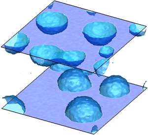Equation (3.16) suggests that $f_w$ cannot in general be assigned independently of fluid bulk free energy $f_b(\rho )$, a prescription that is often ignored in applications. In figure 4 we show the equilibrium configurations of a two-dimensional vapour bubble laying on a flat wall with two different wettabilities. In both cases the contact angle $\phi$ has been imposed through the boundary condition for the density field, (3.8). The critical density isoline forms the prescribed contact angle with the solid wall, as expected.

Figure 4. (a) Adsorption/depletion of the density field occurring in the wall-normal direction, $z$, as a function of the contact angle. In the main panel the bulk liquid density is $\rho _b=0.48$. All the quantities are expressed in Lennard-Jones units, as will be explained in § 9. Hydrophobic walls, $\phi > 90^\circ$, show a reduction of the density close to the wall; the opposite behaviour is provided by hydrophilic walls. The inset shows that this layering effect is amplified when the degree of metastability is increased. (b) Vapour–liquid contact angle for hydrophobic (top) and hydrophilic (bottom) solid surfaces.

The proposed fluid–solid free energy describes density layering at the solid surface for non-neutrally wettable surfaces ($\cos \phi \ne 0$). Layering is a common feature for liquids in contact with solid walls. At nanoscale, oscillations of the density field close to the wall are known to occur, as observed through X-ray scattering experiments (Huisman et al. Reference Huisman, Peters, Zwanenburg, de Vries, Derry, Abernathy and van der Veen1997Reference Ito, Lhuissier, Wildeman and Lohse; Yu et al. Reference Yu, Richter, Datta, Durbin and Dutta2000) or MD simulations (Sikkenk et al. Reference Sikkenk, Indekeu, Van Leeuwen and Vossnack1987). They are well captured by the intrinsically non-local DFT (Tarazona & Evans Reference Tarazona and Evans1984; Tarazona, Marini Bettolo Marconi & Evans Reference Tarazona, Marini Bettolo Marconi and Evans1987; Evans, Stewart & Wilding Reference Evans, Stewart and Wilding2017). The possible effect on nucleation of these near-wall density oscillations cannot be addressed in the present framework, which, due to the intrinsic limitations of purely local theories, should be understood as a coarse-grained description of the actual phenomenology, resulting in a monotonic density layering at the wall. A related approach is described in (Carey & Wemhoff Reference Carey and Wemhoff2005), where the fluid–solid interaction is accounted for through an interaction potential between solid and fluid particles, leading, through a mean-field theory, to a disjoining pressure, which induces a similar monotonic density stratification at the wall.

In the hydrophilic case, the liquid–solid interaction accumulates fluid at the wall, resulting in a local increase of density. Conversely, the lower affinity of hydrophobic walls produces a depletion region with layers of the order of a few nanometres – see figure 4 reporting the density profiles obtained by applying the boundary condition (3.8) for different wetting properties of the surface. This aspect is important for heterogeneous nucleation, since it facilitates the process at hydrophobic walls while discouraging it on hydrophilic surfaces (see the more detailed discussion in § 9).

4. The capillary Navier–Stokes model

Aim of the present section is deriving constitutive relations for stresses and energy fluxes consistent with the Clausius–Duhem formulation of thermodynamic irreversibility (De Groot & Mazur Reference De Groot and Mazur2013) for non-homogeneous, wall-bounded capillary systems – see Magaletti et al. (Reference Magaletti, Gallo, Marino and Casciola2016) for the case of a homogeneous fluid.

The theory explicitly takes into account capillary effects occurring in the fluid, not only at the vapour–liquid interface but also in the stratified layer close to a substrate (typically, a solid wall). Stratification at a substrate is induced by the combination of capillarity (the $\lambda |\boldsymbol {\nabla } \rho |^2$ contribution to the free energy (3.1)) and surface free energy $f_w(\rho ,\theta )$ included in the boundary contribution. Associated with the surface free energy term there is a surface entropy with density $s_w = - \partial f_w/\partial \theta$. In order to account for possible additional entropy production terms arising from the wall potential, the system can be thought of as comprising fluid, solid and a concentrated, zero-thickness layer separating fluid and solid. In total generality the layer may possess a (concentrated) mass density $\rho _w$ (units of mass per unit area) and a velocity $\boldsymbol {v}_w$, hence a kinetic energy density $\frac 12 \rho _L \vert \boldsymbol {v}_w \vert ^2$, and a total surface energy density, the sum of internal, $u_w = f_w + \theta \partial f_w/\partial \theta$, and kinetic energy density. The surface free energy density is assumed to depend on the mass density of the fluid in contact with the layer $\rho$, on the concentrated mass density associated with the layer $\rho _w$ and on temperature. The equations for the layer establish mass, momentum and energy conservation, and will be used in the limit of vanishing layer mass density, $\rho _w$, such that, in the limit, the surface potential recovers the form $f_w(\rho ,\theta )$. In order not to burden the discussion, the governing equations inside the layer will be described in detail in appendix A. Here, only the results of the procedure are reported, consisting of a relaxation condition for the contact angle in the diffuse capillary context.

For a capillary fluid enclosed in a volume ${\mathcal {D}}$, the conservation laws for mass $M$, momentum $\boldsymbol {P}$ and total energy $E$ are (the inclusion of mass forces is straightforward)

(4.1)\begin{equation} \left.\begin{array}{c@{}} \displaystyle\dfrac{\textrm{d} M}{\textrm{d} t} = \dfrac{\textrm{d} }{\textrm{d} t}\int_{\mathcal{D}} \rho \, \textrm{d} V= 0 , \\ \displaystyle\dfrac{\textrm{d} \boldsymbol{P}}{\textrm{d} t} = \dfrac{\textrm{d} }{\textrm{d} t}\int_{\mathcal{D}} \rho\boldsymbol{v} \, \textrm{d} V = \int_{\partial {\mathcal{D}}} \boldsymbol{\varSigma}\boldsymbol{\cdot} \boldsymbol{n} \, \textrm{d} S , \\ \displaystyle\dfrac{\textrm{d} E}{\textrm{d} t} = \dfrac{\textrm{d} }{\textrm{d} t}\int_{\mathcal{D}} e \, \textrm{d} V = \int_{\partial {\mathcal{D}}} (\boldsymbol{\varSigma} \boldsymbol{\cdot} \boldsymbol{v}-\boldsymbol{q})\boldsymbol{\cdot} \boldsymbol{n} \, \textrm{d} S , \end{array}\right\} \end{equation}

where $\boldsymbol {n}$ is the outward unit vector normal to the boundary, $\boldsymbol {v}$ is the fluid velocity, $e=u+\frac 12 \rho \vert \boldsymbol {v}\vert ^2$ is the total energy density, with $u=u_b+u_c$ the internal energy density defined in (3.4), and $\boldsymbol {\varSigma }$ and $\boldsymbol {q}$ the are stress tensor and heat flux, respectively, to be determined in the following. The local form of the conservation laws is obtained by applying Green's theorem, and take the classical form

(4.2)\begin{equation} \left.\begin{array}{c@{}} \displaystyle \dfrac{\partial \rho}{\partial t}+ \boldsymbol{\nabla}\boldsymbol{\cdot}\left( \rho\boldsymbol{v}\right) = 0 , \\ \displaystyle \dfrac{\partial \rho\boldsymbol{v}}{\partial t}+ \boldsymbol{\nabla}\boldsymbol{\cdot}\left( \rho\boldsymbol{v}\otimes\boldsymbol{v}\right) = \boldsymbol{\nabla}\boldsymbol{\cdot}\boldsymbol{\varSigma} ,\\ \displaystyle \dfrac{\partial e}{\partial t}+ \boldsymbol{\nabla}\boldsymbol{\cdot}( \boldsymbol{v} e) = \boldsymbol{\nabla}\boldsymbol{\cdot}( \boldsymbol{\varSigma}\boldsymbol{\cdot}\boldsymbol{v} -\boldsymbol{q}) . \end{array}\right\} \end{equation}

Under the assumption of local equilibrium, the above equations can be manipulated, as usual in the context of non-equilibrium thermodynamics (De Groot & Mazur Reference De Groot and Mazur2013), to obtain an evolution equation for the entropy density. Namely, the internal energy evolution is first derived by subtracting the kinetic energy contribution from the total energy density,

(4.3)\begin{equation} \rho\frac{\textrm{D} \tilde{u}}{D t } - \boldsymbol{\varSigma} \boldsymbol{:} \boldsymbol{\nabla} \boldsymbol{v} + \boldsymbol{\nabla} \boldsymbol{\cdot} \boldsymbol{q} = 0, \end{equation}

where $\textrm {D}/\textrm {D}t = \partial /\partial t + \boldsymbol {v}\boldsymbol {\cdot } \boldsymbol {\nabla }$ is the material derivative and $\tilde {u} = u/\rho$ is the specific internal energy. By definition $\tilde {u} = \tilde {f} + \theta \tilde {s}$, with $\tilde {f} = (\,f_b + (\lambda /2)\vert \boldsymbol {\nabla }\rho \vert ^2)/\rho$ – see (3.1) and comments below – and hence its differential reads

(4.4)\begin{equation} {\mathrm d} \tilde{u} = \dfrac{\partial \tilde{f}}{\partial \rho}{\mathrm d}\rho + \dfrac{\partial \tilde{f}}{\partial \boldsymbol{\nabla}\rho}\boldsymbol{\cdot}{\mathrm d}\boldsymbol{\nabla}\rho + \theta\, {\mathrm d}\tilde{s}. \end{equation}

The partial derivatives of the specific free energy are derived from its definition, (3.1), providing

(4.5)\begin{equation} \rho \frac{\textrm{D} \tilde{u}}{\textrm{D} t} = \frac{1}{\rho}\left(p-\frac{\lambda}{2}\vert\boldsymbol{\nabla}\rho\vert^2\right) \frac{\textrm{D} \rho}{\textrm{D} t} + \lambda\boldsymbol{\nabla}\rho\boldsymbol{\cdot} \frac{\textrm{D} \boldsymbol{\nabla}\rho}{\textrm{D}t} + \rho\theta\frac{\textrm{D} \tilde{s}_b}{\textrm{D} t} , \end{equation}

with $p$ the pressure. The material derivative of the density gradient (second term on the right-hand side of (4.5)) is evaluated from the mass conservation equation (Magaletti et al. Reference Magaletti, Gallo, Marino and Casciola2016),

(4.6)\begin{equation} \lambda \boldsymbol{\nabla}\rho\boldsymbol{\cdot} \frac{\textrm{D} \boldsymbol{\nabla}\rho}{\textrm{D}t} = \boldsymbol{\nabla}\boldsymbol{\cdot}\left(\lambda \boldsymbol{\nabla}\rho \frac{\textrm{D} \rho}{\textrm{D}t}\right) - \lambda \nabla^2 \rho \boldsymbol{\nabla}\rho \frac{\textrm{D} \rho}{\textrm{D}t} - \lambda \boldsymbol{\nabla}\rho \otimes \boldsymbol{\nabla}\rho \boldsymbol{:} \boldsymbol{\nabla}\boldsymbol{v}. \end{equation}

After substitution of (4.5) and (4.6) into (4.3), a few more elementary steps isolate the entropy time derivative as

(4.7)\begin{align} \rho \frac{\textrm{D} \tilde{s}}{\textrm{D} t} &= -\boldsymbol{\nabla}\boldsymbol{\cdot}\left[\frac{1}{\theta} \left(\lambda\boldsymbol{\nabla}\rho \frac{\textrm{D} \rho}{\textrm{D}t} + \boldsymbol{q}\right) \right] - \left[ \lambda \boldsymbol{\nabla}\rho \frac{\textrm{D} \rho}{\textrm{D}t}+ \boldsymbol{q}\right] \boldsymbol{\cdot}\frac{\boldsymbol{\nabla}\theta}{\theta^2} \nonumber\\ &\quad + \left[\boldsymbol{\varSigma} + \left(p - \frac{\lambda}{2}\lvert \boldsymbol{\nabla}\rho\rvert^2 - \lambda \rho\nabla^2 \rho \right) {\boldsymbol{\mathsf{I}}} + \lambda \boldsymbol{\nabla} \rho\otimes\boldsymbol{\nabla}\rho\right]\boldsymbol{:} \frac{\boldsymbol{\nabla}\boldsymbol{v}}{\theta} , \end{align}

where the divergence of the entropy flux (first term on the right-hand side) and two entropy production terms appear. By requiring a positive entropy production (Clausius–Duhem inequality) and by restricting the analysis to linear constitutive prescriptions for stress

(4.8)\begin{align} \boldsymbol{\varSigma} &= \boldsymbol{\varSigma}_{rev} + \boldsymbol{\varSigma}_{v} \nonumber\\ &= \left(-p + \frac{\lambda}{2}\vert\boldsymbol{\nabla}\rho\vert^2 + \lambda\rho\nabla^2\rho\right) {\boldsymbol{\mathsf{I}}} - \lambda\boldsymbol{\nabla}\rho\otimes\boldsymbol{\nabla}\rho + \eta\left[(\boldsymbol{\nabla}\boldsymbol{u} + \boldsymbol{\nabla}\boldsymbol{u}^\textrm{T}) - \frac{2}{3}\boldsymbol{\nabla} \boldsymbol{\cdot}{u}{\boldsymbol{\mathsf{I}}}\right] \end{align}

and energy flux

(4.9)\begin{equation} \boldsymbol{q} = \boldsymbol{q}_c + \boldsymbol{q}_h = - \lambda \boldsymbol{\nabla}\rho\frac{\textrm{D} \rho}{\textrm{D}t} - k \boldsymbol{\nabla}\theta, \end{equation}

capillary effects are explicitly included in the model. The irreversible part of the stress is the classical Newtonian viscous tensor, where $\eta >0$ is the dynamic viscosity. Since viscosity is not expected to play a crucial role in nucleation (e.g. in CNT it is completely neglected), the simplest choice $-2 \eta /3$ is made here for the second viscosity coefficient. A general value can be, however, straightforwardly included in the model as needed, e.g. to describe damping in nonlinear bubble oscillations (Scognamiglio et al. Reference Scognamiglio, Magaletti, Izmaylov, Gallo, Casciola and Noblin2018). Similarly, the classical Fourier's heat flux, with $k>0$ the thermal conductivity, provides the irreversible part of the energy flux. It is worth noting that the capillary (square density gradient) term in the free energy leads to capillary stresses included in the reversible part of the dynamics (no entropy production), as expected from the general thermodynamic definition of surface tension.

The field equations for a capillary fluid, (4.2), (4.8) and (4.9), require an additional boundary condition for the density field. The equilibrium considerations of § 3 suggest the density normal derivative as the appropriate prescription, (3.8). This result can be extended to non-equilibrium conditions through a procedure strictly similar to that just reviewed for the bulk, applied in this case to the layer adjoining the fluid and solid surface. The layer is described in terms of suitable fields defined on the manifold supporting the layer that are energetically, mechanically and kinematically coupled with the neighbouring fluid. By prescribing that each entropy production term is non-negative (Clausius–Duhem inequality combined with Curie principle), linear constitutive laws for the layer stress tensor ${\boldsymbol{\mathsf{Q}}}_{\boldsymbol\pi}$ and for the layer tangential heat flux $\boldsymbol {q}_w$ are derived (see appendix A for derivation details).

The requirement that the entropy production associated with the layer should, in general, be non-negative leads to relaxing the equilibrium wetting condition. In this more general setting, the prescription of the equilibrium (Young) contact angle, (3.8), is replaced by the boundary equation

(4.10)\begin{equation} \dfrac{\textrm{D} \rho}{\textrm{D} t} = - D_w\left( \frac{\partial f_w}{\partial \rho} + \lambda \dfrac{\partial \rho}{\partial n} \right) , \end{equation}

where $D_w$ is a mobility coefficient determining the relaxation time scale. Notice that the surface free energy $f_w$, as an equilibrium property of the system, keeps the form (3.16) obtained in § 3. This equation describes the relaxation of the contact angle towards equilibrium and can be understood as a generalization to the non-isothermal case and to general equations of state for the bulk fluid of the contact angle dynamics proposed in Jacqmin (Reference Jacqmin2000), Carlson, Do-Quang & Amberg (Reference Carlson, Do-Quang and Amberg2009, Reference Carlson, Do-Quang and Amberg2011) and Ren & E (Reference Ren and E2011). In what follows, the boundary term associated with (4.10) will be assumed to provide a negligible contribution to the entropy, implying the equilibrium Young's law (3.15).

5. Equilibrium thermal fluctuations of a wall-bounded capillary fluid

Fluids at a mesoscopic scale are subject to thermal fluctuations that need to be included in the hydrodynamic equations. The purpose of this section is discussing thermal fluctuations for a capillary fluid in contact with a solid surface. What follows falls within the theoretical framework of fluctuating hydrodynamics, first proposed by Landau & Lifshitz (Reference Landau and Lifshitz1980 reprint) and systematically developed since then (Fox & Uhlenbeck Reference Fox and Uhlenbeck1970; Zubarev & Morozov Reference Zubarev and Morozov1983; Español et al. Reference Español, Anero and Zúñiga2009). The theory was retraced and exploited in the context of liquid–vapour systems far from boundaries to address homogeneous bubble nucleation in a recent work (Gallo et al. Reference Gallo, Magaletti and Casciola2018). The extension of this theory to heterogeneous systems bounded by solid walls is presented here. The focus here is on a fluid enclosed between two fixed rigid solid walls to provide the static correlation functions of the fluid-phase fluctuations. In comparison with the unbounded cases, the interaction with the solid influences the fluctuating fluid field through the boundary conditions.

Equilibrium thermal fluctuations were originally described by Einstein (Reference Einstein1956), who provided the static correlation functions as a result of the entropy deviations ${\rm \Delta} S$ from equilibrium, where the entropy $S_{eq}$ is a maximum. For the system described in § 4, the entropy consists of two contributions: the fluid, $S_f$, and the layer entropy, $S_w$, respectively. In § 3 the entropy deviation was expressed as a functional of mass density, $\delta \rho (\boldsymbol x,t)$, velocity, $\delta {\boldsymbol v}(\boldsymbol x,t)$, and temperature, $\delta \theta (\boldsymbol x,t)$, fluctuations (see (3.3)).

Assuming small fluctuations with respect to the mean field, the entropy – a functional of the mass density, velocity and temperature fields – can be Taylor-expanded to second order around equilibrium (second order at least is required, since at equilibrium the first variation vanishes altogether). Explicitly, using the variables $\boldsymbol {U} = (\rho , \boldsymbol {\nabla }\rho , \theta , \boldsymbol {v})^\textrm {T}$, where field derivatives higher than the density gradient will not be needed since the free energy (3.1) is quadratic in the density gradients, the entropy functional is

(5.1)\begin{align} {\rm \Delta} S_c &= S_c -S_{eq} = \int_{V}{\rm \Delta} s_{c f} (\rho, \boldsymbol{\nabla}\rho, \theta, \boldsymbol v)\, \textrm{d} V + \oint_{\partial V}{\rm \Delta} s_{c w} (\rho, \theta, \boldsymbol v)\, \textrm{d} S \nonumber\\ &= \left.\int_{V} \frac{1}{2}\,\sum_{i,j} \frac{\partial^2 {\rm \Delta} s_c }{\partial U_i \partial U_j}\right\vert_{eq} \delta U_i \delta U_j \, \textrm{d} V + \left.\oint_{\partial V} \frac{1}{2}\,\sum_{i,j} \frac{\partial^2 {\rm \Delta} s_{c w} }{\partial U_i \partial U_j}\right\vert_{eq} \delta U_i \delta U_j \, \textrm{d} S \nonumber\\ &= {\rm \Delta} S_{c f} + {\rm \Delta} S_{c w} . \end{align}

Exploiting the well-known relations (the subscript b stands for homogeneous bulk conditions where capillary contributions do not appear)

(5.2)\begin{equation} \left.\begin{array}{c@{}} \displaystyle \mathrm{d} s_b = \dfrac{1}{\theta}\,\mathrm{d} u_b - \dfrac{\mu_b}{\theta}\,\mathrm{d}\rho ,\\ \displaystyle \mathrm{d} u_b = \rho c_{v}\,\mathrm{d}\theta+\left(\mu_b+\theta\left. \dfrac{\partial s_b}{\partial\rho}\right\vert_\theta\right)\, \mathrm{d}\rho, \\ \displaystyle \mathrm{d}\mu_b = \dfrac{c_{T}^{2}}{\rho}\,\mathrm{d}\rho+\left(\dfrac{1}{\rho} \left.\dfrac{\partial p}{\partial\theta}\right\vert_\rho-\dfrac{s_b}{\rho}\right)\, \mathrm{d}\theta , \end{array}\right\} \end{equation}

where $c_{v}$ is the constant-volume specific heat and $c_{T}$ is the isothermal speed of sound, (5.1) can be rearranged as

(5.3)\begin{align} {\rm \Delta} S_c &= -\frac{1}{2} \int_V \left[ \frac{c_{T, eq}^{2}}{\theta_{eq}\rho_{eq}}\delta\rho^{2}-\frac{\lambda}{\theta_{eq}} \delta\rho (\nabla^2\delta\rho ) \right] \textrm{d} V \nonumber\\ &\quad - \frac{1}{2} \int_V \left[ \frac{\rho_{eq}}{\theta_{eq}}\delta\boldsymbol{v}\boldsymbol{\cdot} \delta\boldsymbol{v}+\frac{\rho_{eq}c_{v,eq}}{\theta_{eq}^{2}} \delta\theta^{2}\right] \textrm{d} V \nonumber\\ &\quad - \frac{1}{2} \oint_{\partial V} \frac{1}{\theta_{eq}}\left[ \lambda \delta\left( \frac{\partial \rho}{\partial n}\right)_{eq} \delta\rho + \left.\frac{\partial^2 f_w}{\partial \rho^2}\right\vert_{eq} \delta\rho^2\right] \textrm{d} S - \frac{1}{2} \oint_{\partial V} \frac{1}{\theta_{eq}} \left.\frac{\partial s_w}{\partial \theta}\right\vert_{eq} \delta\theta^2 \, \textrm{d} S . \end{align}

The first two rows are the volume contributions already discussed in

Gallo et al. (Reference Gallo, Magaletti and Casciola2018). The new terms on the third line arise from the solid–liquid interaction due to the layer entropy. The first integral in the third row of (5.3) has two different contributions: the first one arises from the integration by parts of the square gradient, and the second comes from the solid–liquid energy $f_w$. As a consequence of the static boundary condition, (3.8), the whole first integral vanishes (see the comments at the end of § 4 and appendix A):

(5.4)\begin{equation} \oint_{\partial V} \lambda \delta\left( \frac{\partial \rho}{\partial n}\right) \delta\rho + \frac{\partial^2 f_w}{\partial \rho^2} \delta\rho^2 \, \textrm{d} S = \oint_{\partial V} \frac{\delta}{\delta \rho} \left[\left(\lambda\boldsymbol{\nabla}\rho \boldsymbol{\cdot} \hat{\boldsymbol{n}} + \frac{\partial f_w}{\partial \rho}\right)\right] \delta\rho \, \textrm{d} S =0 . \end{equation}

Fluctuating field correlations are most easily obtained after recasting the entropy in a form more appropriate to operational manipulations:

(5.5)\begin{align} {\rm \Delta} S_c & = -\frac{1}{2} \int_{V} \int_{V} \textrm{d} V_{\boldsymbol x} \, \textrm{d} V_{\tilde {\boldsymbol x}} \left\{\delta {\boldsymbol v}({\boldsymbol x}) \frac{\rho_{eq}}{\theta_{eq}} \delta({\boldsymbol x} - {\tilde {\boldsymbol x}} ) \boldsymbol{\cdot} \delta {\boldsymbol v}({\tilde {\boldsymbol x}}) \right. \nonumber\\ &\quad +\delta\rho({\boldsymbol x}) \left[\frac{c_{T,eq}^{2}}{\theta_{eq}\rho_{eq}} \delta({\boldsymbol x} - {\tilde {\boldsymbol x}} ) -\frac{\lambda}{\theta_{eq}} \nabla_{\boldsymbol x}^2 \delta({\boldsymbol x} - {\tilde {\boldsymbol x}} ) \right] \delta\rho({\tilde {\boldsymbol x}}) \nonumber\\ &\quad \left.+ \, \delta \theta({\boldsymbol x}) \frac{\rho_{eq} c_{v,eq}}{\theta_0^2} \delta({\boldsymbol x} - {\tilde {\boldsymbol x}} ) \delta \theta({\tilde {\boldsymbol x}}) \right\} \nonumber\\ &\quad -\frac{1}{2} \oint_{\partial V}\oint_{\partial V} \textrm{d} S_{ {\boldsymbol{ x}}_w} \, \textrm{d} S_{\tilde {\boldsymbol x}_w}\left[ \delta \theta({\boldsymbol x}_w) \left.\frac{\partial s_w}{\partial \theta} \right\vert_{eq}\delta_w({\boldsymbol x}_w - {\tilde {\boldsymbol x}_w} ) \delta \theta({\tilde {\boldsymbol x}_w})\right] . \end{align}

In the above equation, $\delta ({\boldsymbol x} - {\tilde {\boldsymbol x}})$ is the ordinary three-dimensional Dirac delta function and $\delta _w({\boldsymbol x}_w - {\tilde {\boldsymbol x}_w} )$ denotes the Dirac delta function on the manifold,

(5.6)\begin{equation} \oint_{\partial V} f({\tilde {\boldsymbol x}_w}) \delta_w({\boldsymbol x}_w - {\tilde {\boldsymbol x}_w} ) \, \textrm{d} S_{\tilde {\boldsymbol x}_w} := \int_{{\mathcal{S}}} \, \textrm{d} S_{\tilde {\boldsymbol \xi}} \,\, f({\tilde {\boldsymbol \xi}}) \delta_{2D}({\boldsymbol \xi} - {\tilde {\boldsymbol \xi}} ), \end{equation}

where ${\boldsymbol x}_w = {\boldsymbol x}_w ({\boldsymbol \xi }) \in \mathbb {R}^3$, ${\boldsymbol \xi } = (\xi ^1,\xi ^2) \in {\mathcal {S}} \subset \mathbb {R}^2$ is the parametric equation (locally) describing the boundary and $\delta _{2D}$ is the ordinary two-dimensional Dirac delta function. Integration by parts is used twice to move the Laplacian $\nabla ^2$ from the density fluctuation $\delta \rho$ to the Dirac delta function. In a compact operator form, (5.5) reads

(5.7)\begin{equation} {\rm \Delta} S_c = {\rm \Delta} S_{c f} + {\rm \Delta} S_{c w} = -\tfrac{1}{2} \int_{V} {\boldsymbol \varDelta}^{\dagger}\boldsymbol{\mathcal{H}}_{\boldsymbol{f}} \,{\boldsymbol \varDelta} \,\textrm{d} V -\tfrac{1}{2} \oint_{\partial V} {\delta \theta}^{\dagger}{\mathcal{H}}_w \,{\delta\theta} \, \textrm{d} S , \end{equation}

with $\boldsymbol {\varDelta } = (\delta \rho ,\delta \boldsymbol {v},\delta \theta )$ denoting the fluctuating fields, and $\boldsymbol{\mathcal{H}}_{\boldsymbol{f}}$ and ${\mathcal {H}}_w$ are diagonal, positive definite operators, defined as

(5.8)\begin{gather} (\boldsymbol{\mathcal{H}}_{\boldsymbol{f}} {\boldsymbol \varDelta})({\boldsymbol x}) = \int_V {\boldsymbol{\mathsf{H}}}_f({\boldsymbol x}, {\tilde {\boldsymbol x}}) {\boldsymbol\varDelta}({ \tilde{\boldsymbol x}} )\,\textrm{d} V_{ \tilde{\boldsymbol x}} = \int_V \hat{\boldsymbol{\mathsf{H}}}_f({\boldsymbol x}) \delta({\boldsymbol x}-{\tilde {\boldsymbol x}}) {\boldsymbol\varDelta}({ \tilde{\boldsymbol x}} )\,\textrm{d} V_{ \tilde{\boldsymbol x}}, \end{gather}

(5.9)\begin{gather}({\mathcal{H}}_w {\delta \theta})({\boldsymbol x}_w) = \oint_{\partial V} {\boldsymbol{\mathsf{H}}}_w({\boldsymbol x}_w, {\tilde {\boldsymbol x}_w}) {\delta\theta}({\tilde {\boldsymbol x}_w}) \, \textrm{d} S_{\tilde {\boldsymbol x}_w} = \oint_{\partial V} \hat{\boldsymbol{\mathsf{H}}}_w({\boldsymbol x}_w) \delta_w({\boldsymbol x}_w-{\tilde {\boldsymbol x}_w}) {\delta \theta }({\tilde {\boldsymbol x}_w}) \, \textrm{d} S_{\tilde {\boldsymbol x}_w}, \end{gather}

where

(5.10)\begin{equation} \boldsymbol {\hat H}_f = \left( \begin{array}{@{}ccc@{}} \dfrac{c_{T,eq}^{2}}{\theta_{eq}\rho_{eq}}-\dfrac{\lambda}{\theta_{eq}}\nabla_{\boldsymbol x}^2 & 0 & 0 \\ 0 & \dfrac{\rho_{eq}}{\theta_{eq}} {\boldsymbol{\mathsf{I}}} & 0 \\ 0 & 0 & \dfrac{\rho_{eq}c_{v,eq}}{\theta_{eq}^{2}} \end{array} \right) \end{equation}

involves differential operators with ${\boldsymbol{\mathsf{I}}}$ the $3 \times 3$ identity matrix and

(5.11)\begin{equation} \hat{\boldsymbol{\mathsf{H}}}_w = \left.\frac{\partial s_w}{\partial \theta} \right\vert_{eq} . \end{equation}

The probability distribution functional for the fluctuating fields $\boldsymbol {\varDelta }$ (Einstein Reference Einstein1956),

(5.12)\begin{equation} P_{eq}[\boldsymbol{\varDelta}]=\frac{1}{Z}\exp\left({\frac{{\rm \Delta} S_c}{k_{B}}}\right) = \frac{1}{Z_f}\exp\left({\frac{{\rm \Delta} S_{c f}}{k_{B}}}\right) \frac{1}{Z_w}\exp\left({\frac{{\rm \Delta} S_{c w}}{k_{B}}}\right), \end{equation}

can be approximated by exploiting the second-order approximation, (5.7),

(5.13)\begin{equation} P_{eq}[{\boldsymbol \varDelta}]=\frac{1}{Z_f}\exp\left({-\frac{1}{2k_{B}} \int_{V}{\boldsymbol \varDelta}^{\dagger}\boldsymbol{\mathcal{H}}_{\boldsymbol{f}}\,{\boldsymbol \varDelta}\,\textrm{d} V} \right) \frac{1}{Z_w}\exp\left({-\frac{1}{2k_{B}}\oint_{\partial V} \delta\theta^{\dagger}{\mathcal{H}}_w\,\delta\theta\,\textrm{d} S} \right). \end{equation}

Owing to the exponential form of the probability distribution functional, the diagonal nature of the operator $\hat {\boldsymbol{\mathsf{H}}}_f$ together with the local dependence on temperature of the entropy, $P_{eq}$ can be factorized as

(5.14)\begin{equation} P_{eq}[{\boldsymbol \varDelta}] = P_f[\boldsymbol{\varDelta}] P_w[\delta\theta] = P_f[\delta\rho] P_f[\delta\boldsymbol{v}] P_f[\delta\theta] P_w[\delta\theta] , \end{equation}

which implies that the fluctuations of temperature in the fluid and in the layer are statistically independent. Focusing on the fluid domain, the relevant property of the probability distribution functional is the correlation function

(5.15)\begin{equation} {\boldsymbol{\mathsf{C}}}_f(\boldsymbol{x}, \tilde{\boldsymbol{x}} ) = \langle\boldsymbol{\varDelta}(\boldsymbol{x})\otimes \boldsymbol{\varDelta}^{\dagger}( \tilde{\boldsymbol{x}} )\rangle = \frac{1}{Z}\int {\mathcal{D}}\boldsymbol{\varDelta} \boldsymbol{\varDelta}(\boldsymbol{x})\otimes \boldsymbol{\varDelta}^{\dagger}( \tilde{\boldsymbol{x}} ) P_{eq} [\boldsymbol{\varDelta} ], \end{equation}

where the integral over all the possible field fluctuations is understood on the right-hand side (path integral). It can be evaluated in closed form given the quadratic approximation for the entropy, which leads to Gaussian path integrals. The final expression is (see Gallo et al. (Reference Gallo, Magaletti and Casciola2018) for details)

(5.16)\begin{equation} {\boldsymbol{\mathsf{C}}}_f (\boldsymbol{x}, \tilde{\boldsymbol{x}} ) = k_B {\boldsymbol{\mathsf{H}}}_f^{-1} (\boldsymbol{x}, \tilde{\boldsymbol{x}}), \end{equation}

implying the following identity:

(5.17)\begin{equation} \int_V {\boldsymbol{\mathsf{H}}}_f (\boldsymbol{x}, \hat{\boldsymbol x}) {\boldsymbol{\mathsf{C}}}_f (\hat{\boldsymbol x}, \tilde{\boldsymbol{x}} ) \, \textrm{d} V_{\hat{\boldsymbol x}} = {\boldsymbol{\mathsf{I}}} k_B \delta (\boldsymbol{x} - \tilde{\boldsymbol{x}}). \end{equation}

From a practical standpoint, the correlation functions are obtained by solving the equivalent equation

(5.18)\begin{equation} \hat{\boldsymbol{\mathsf{H}}}_f(\boldsymbol{x}) {\boldsymbol{\mathsf{C}}}_f(\boldsymbol{x}, \tilde{\boldsymbol{x}}) = {\boldsymbol{\mathsf{I}}} k_B \delta (\boldsymbol{x} - \tilde{\boldsymbol{x}}) \end{equation}

(recall that ${\boldsymbol{\mathsf{H}}}_f (\boldsymbol { x}, \hat {\boldsymbol x})$ and $\hat {\boldsymbol{\mathsf{H}}}_f(\boldsymbol { x})$ are slightly different objects, (5.8)). The velocity and temperature correlations at equilibrium are straightforwardly obtained as

(5.19)\begin{gather} {\boldsymbol{\mathsf{C}}}_f^{{\delta \boldsymbol{v} \delta \boldsymbol{v}}} (\boldsymbol{x}, \tilde{\boldsymbol{x}}) = \frac{k_B \theta_{eq}} {\rho_{eq}} \delta(\boldsymbol{x} - \tilde{\boldsymbol{x}}) {\boldsymbol{\mathsf{I}}}, \end{gather}

(5.20)\begin{gather}{\boldsymbol{\mathsf{C}}}_f^{\delta \theta \delta \theta}(\boldsymbol{x}, \tilde{\boldsymbol{x}}) = \frac{k_B \theta_{eq}^2} {c_{v,eq}} \delta (\boldsymbol{x} - \tilde{\boldsymbol{x}}), \end{gather}

respectively. The density correlation involves instead a differential operator, calling for the solution of the differential equation

(5.21)\begin{equation} \left(\frac{c_{T,eq}^{2}}{\theta_{eq}\rho_{eq}} -\frac{\lambda}{\theta_{eq}}\nabla_{\boldsymbol x}^2\right) { {\boldsymbol{\mathsf{C}}}_f^{{\delta \rho \delta \rho}}} (\boldsymbol{x}, \tilde{\boldsymbol{x}}) = k_B \delta (\boldsymbol{x} - \tilde{\boldsymbol{x}}), \end{equation}

complemented with the boundary conditions specifying the wall wettability. Since the linearized form of (3.8) reads

(5.22)\begin{equation} \left.\lambda\frac{\partial \delta\rho}{\partial n} + \frac{\partial^2 f_w}{\partial \rho^2}\right\vert_{eq} \delta\rho = 0, \end{equation}

the boundary conditions for the density–density correlation ${\boldsymbol{\mathsf{C}}}_f^{\delta \theta \delta \theta } = \langle \delta \rho (\boldsymbol {x}) \delta \rho (\tilde {\boldsymbol {x}}) \rangle$, i.e. the Green's function in (5.21), is

(5.23)\begin{equation} \left.\lambda\frac{\partial {{\boldsymbol{\mathsf{C}}}_f^{{\delta \rho \delta \rho}}} (\boldsymbol{x}, \tilde{\boldsymbol{x}})}{\partial n_{\boldsymbol x}} + \frac{\partial^2 f_w}{\partial \rho^2}\right\vert_{eq} { {\boldsymbol{\mathsf{C}}}_f^{{\delta \rho \delta \rho}}}(\boldsymbol{x}, \tilde{\boldsymbol{x}}) = 0. \end{equation}

At variance with the unbounded system (Gallo et al. Reference Gallo, Magaletti and Casciola2018), a closed-form solution of (5.21) is not readily available in the presence of the solid wall, because of the inhomogeneity of the coefficients ($C_{T,eq} = C_{T,eq}(\boldsymbol {x})$) in the linear equation for the Green's function, due to the stratification of the equilibrium density at the wall, $\rho _{eq} = \rho _{eq}(\boldsymbol {x})$, which exists whenever the equilibrium contact angle differs from $90^\circ$ (neutral wettability).

6. Fluctuation–dissipation balance for wall-bounded capillary fluids: general theory

In a nutshell, fluctuating hydrodynamics amounts to including suitable stochastic forcing terms into the linearized version of the field equations. The noise is assumed to be generated by a linear operator (noise operator) acting on a zero-mean, delta-correlated-in-time Gaussian process (white noise). The equilibrium solution of the resulting system of SPDEs is a Gaussian field, completely determined by the correlations. After the noise operator is determined in such a way to generate the equilibrium correlations independently defined in terms of the entropy functional, the resulting SPDEs will sample the Gaussian equilibrium probability functional $P_f[\boldsymbol {\varDelta }]$ discussed in the previous section. In other words, once the equilibrium correlation functions of the fluctuating fields are known, the fluctuation–dissipation balance (FDB) provides the explicit form of the stochastic forcing. Eventually, the capillary Navier–Stokes equations (4.2) and (4.8) completed with the additional stochastic contributions (4.9) result in a model that could be dubbed the capillary Landau–Lifshitz–Navier–Stokes (CLLNS) system. The purpose of the present section is to extend this model to the case of a wall-bounded capillary fluid. As will be shown in detail, the FDB can be satisfied keeping the noise in the form of a standard white noise. The noise terms act on momentum and energy and, also in the presence of walls, keeps the divergence form, consistently with the expected conservation properties. Special care is devoted to include the appropriate boundary conditions in the relevant operators, a crucial point in order to avoid the need to modify the structure of the noise.

The three-dimensional CLLNS system augmented with noise is

(6.1)\begin{equation} \left.\begin{array}{c@{}} \dfrac{\partial\rho}{\partial t}+ \boldsymbol{\nabla}\boldsymbol{\cdot}( \rho\boldsymbol{v}) = 0 , \\ \dfrac{\partial\rho\boldsymbol{v}}{\partial t}+ \boldsymbol{\nabla}\boldsymbol{\cdot}( \rho\boldsymbol{v}\otimes\boldsymbol{v}) = \boldsymbol{\nabla}\boldsymbol{\cdot}\boldsymbol{\varSigma} + \boldsymbol{f}_\varSigma ,\\ \dfrac{\partial E}{\partial t}+ \boldsymbol{\nabla}\boldsymbol{\cdot}( \boldsymbol{v} E) = \boldsymbol{\nabla}\boldsymbol{\cdot}( \boldsymbol{v}\boldsymbol{\cdot}\boldsymbol{\varSigma} -\boldsymbol{q} ) + \boldsymbol{v}\boldsymbol{\cdot}\boldsymbol{f}_\varSigma + f_q , \end{array}\right\} \end{equation}

where $E$ is the total energy density, $E = {\mathcal {U}} + \frac 12 \rho \vert \boldsymbol {v}\vert ^2 + \frac 12 \lambda \vert \boldsymbol {\nabla }\rho \vert ^2$, with ${\mathcal {U}}$ the internal energy density. In the momentum and energy equations, respectively, $\boldsymbol \varSigma$ and $\boldsymbol q$ are the classical deterministic stress tensor and energy flux (derived in § 4), respectively. The boundary conditions consist of the no-slip/impermeability condition for velocity, zero heat flux and prescribed wall wettability at the solid surface:

(6.2a–c)\begin{equation} \rho \boldsymbol{v} = 0, \quad \boldsymbol{q}_h \boldsymbol{\cdot} \hat{\boldsymbol{n}} = 0, \quad \lambda\boldsymbol{\nabla}\rho\boldsymbol{\cdot}\hat{\boldsymbol{n}} + \frac{\partial f_w}{\partial \rho} = 0. \end{equation}

The stochastic forces, whose statistical properties are to be inferred from the fluctuation–dissipation theorem, are $\boldsymbol {f}_\varSigma$ and $f_q$. After introducing the equilibrium state $\boldsymbol {U}_{eq} =(\rho _{eq}(\boldsymbol {x}), \boldsymbol {0}, \theta _{eq})$ and denoting the fluctuating fields by $\boldsymbol {\varDelta } = (\delta \rho ,\delta \boldsymbol {v},\delta \theta )$, as previously, the state is described by $\boldsymbol {U} = \boldsymbol {\varDelta } + \boldsymbol {U}_{eq}$. With this notation, equations (6.1) written in a compact form are

(6.3)\begin{equation} \left.\begin{array}{c@{}} \dfrac{\partial \boldsymbol{U}}{\partial t} = {\boldsymbol N}[ \boldsymbol{U} ] + \boldsymbol{f}, \quad \boldsymbol{x}\in {\mathcal{D}}, \\ \boldsymbol B [\boldsymbol U] = 0 \quad \boldsymbol{x} \in \partial {\mathcal{D}} , \end{array}\right\} \end{equation}

with $\boldsymbol B$ the operator that specifies the boundary conditions. Linearization around the equilibrium state $\boldsymbol {U}_{eq}$ leads to

(6.4)\begin{align} \left.\begin{array}{c@{}} \dfrac{\partial\delta\rho}{\partial t} = - \boldsymbol{\nabla}\boldsymbol{\cdot}( \rho_{eq} \delta\boldsymbol{v}) , \\ \dfrac{\partial\rho_{eq}\delta\boldsymbol{v}}{\partial t} = - \rho_{eq} \boldsymbol{\nabla}\left( \dfrac{c_{eq}^2}{\rho_{eq}} - \lambda\nabla^2 \right)\delta\rho + \eta\nabla^2\delta{\boldsymbol v} + \dfrac{1}{3}\eta\boldsymbol{\nabla}\boldsymbol{\nabla}\boldsymbol{\cdot} \delta\boldsymbol v - \boldsymbol{\nabla}(\partial_\theta p\vert_{eq} \delta\theta) + \boldsymbol{f}_\varSigma ,\\ \dfrac{\partial c_{v,eq}\rho_{eq} \delta\theta}{\partial t} = - \theta_{eq} \partial_{\theta}p\vert_{eq}\boldsymbol \nabla \boldsymbol{\cdot} \delta\boldsymbol{v} + k \nabla^2\delta\theta + f_q . \end{array}\right\} \end{align}

The linearized system can be rewritten in conservative (divergence) form with the change of variables ${\boldsymbol \varDelta }' = (\delta \rho , \rho _{eq} \delta \boldsymbol {v}, c_{v,eq}\rho _{eq} \delta \theta ) = (\delta \rho , \delta {\boldsymbol \pi }, \delta \iota )$,

(6.5)\begin{equation} \left.\begin{array}{c@{}} \dfrac{\partial \boldsymbol{\varDelta}'}{\partial t} = \boldsymbol{\mathcal{L}} \boldsymbol{\varDelta}' + \boldsymbol{f}, \quad \boldsymbol{x} \in {\mathcal{D}}, \\ \boldsymbol{\mathcal{B}} \boldsymbol{\varDelta}' = 0, \quad \boldsymbol{x} \in \partial {\mathcal{D}} , \end{array}\right\} \end{equation}

where the (linearized) hydrodynamic operator $\boldsymbol {\mathcal {L}}$ is

(6.6)\begin{equation} \boldsymbol{\mathcal{L}}=\left(\begin{array}{@{}ccc@{}} 0 & - \boldsymbol \nabla \boldsymbol{\cdot} & 0\\ -\rho_{eq}\boldsymbol \nabla \left( \dfrac{c_{T,eq}^2}{\rho_{eq}} - \lambda \nabla^2 \right) & {\eta}\left( \nabla^2 + \dfrac{1}{3} \boldsymbol \nabla \boldsymbol \nabla \boldsymbol{\cdot} \right)\dfrac{1}{\rho_{eq}} & -\boldsymbol \nabla \left(\partial_{\theta}p\vert_{eq} \dfrac{1}{\rho_{eq} c_{v,eq}} \right) \\ 0 & -\theta_{eq} \partial_{\theta}p\vert_{eq} \boldsymbol \nabla \boldsymbol{\cdot} \dfrac{1}{\rho_{eq}} & k \nabla^2 \dfrac{1}{\rho_{eq}c_{v,eq}} \end{array}\right) , \end{equation}

and $\boldsymbol {\mathcal {B}}$ is the (linearized) boundary conditions operator

(6.7a,b)\begin{equation} \left.\lambda\frac{\partial \delta\rho}{\partial n} + \frac{\partial^2 f_w}{\partial \rho^2}\right\vert_{eq} \delta \rho = 0,\quad \delta{\boldsymbol \pi} = \boldsymbol {0} , \quad \lambda \frac{\partial \rho_{eq}}{\partial n} \boldsymbol{\nabla}\boldsymbol{\cdot}\delta {\boldsymbol \pi} + k \frac {\partial}{\partial n} \left( \frac{\delta {\iota}}{c_{v eq}\rho_{eq}} \right)= 0 . \end{equation}

The stochastic contribution can be written through the linear operator $\boldsymbol {\mathcal {K}}$ acting on independent white noise processes ${\boldsymbol \varXi }$, as $\boldsymbol f = \boldsymbol {\mathcal {K}} {\boldsymbol \varXi }$, where

(6.8)\begin{equation} \boldsymbol{\mathcal{K}} = \left(\begin{array}{ccc} 0 & 0 & 0\\ 0 & \boldsymbol{\sigma}_{\boldsymbol\pi} & 0\\ 0 & 0 & \sigma_{\iota} \end{array}\right) . \end{equation}

In three dimensions ${\sigma _{\pi }}$ is a $3 \times 3$ matrix whose components are scalar linear operators to be determined. The vector ${\boldsymbol \varXi } = (\varXi^\rho , {\boldsymbol \varXi }^\pi , \varXi^\iota )^\textrm {T}$ collects the white noise processes for the fluctuating fields, with ${\boldsymbol \varXi }^\pi = ( \varXi^{\pi _x}, \varXi^{\pi _y}, \varXi^{\pi _z} )^\textrm {T}$. The Gaussian process ${\boldsymbol \varXi }$ has zero mean and correlations given by

(6.9)\begin{equation} \langle{\boldsymbol \varXi}( \tilde{\boldsymbol{y}},s) \otimes {\boldsymbol \varXi}^\textrm{T}(\hat{\boldsymbol y},q)\rangle = {\boldsymbol{\mathsf{I}}} \delta(\tilde{\boldsymbol{y}} - \hat{\boldsymbol y}) \delta(s-q) , \end{equation}

with ${{\boldsymbol{\mathsf{I}}}}$ now indicating a $( 5 \times 5 )$ identity matrix in ${\boldsymbol \varXi }$ space, $\tilde {\boldsymbol {y}}$ and $\hat {\boldsymbol y}$ denoting space points, and $s$ and $q$ time instants. It may be worth recalling that spatial and temporal Dirac delta functions carry dimensions of reciprocal space and time, respectively. Hence the noise ${\boldsymbol \varXi }$ has dimensions of reciprocal square root of time per volume.

Introducing the operator ${\boldsymbol{\mathsf{L}}}$, which accounts for the differential operator (6.6) completed with the boundary conditions (6.7a,b), problem (6.5) is compactly rewritten as $\textrm {d} \boldsymbol {\varDelta }'/\textrm {d} t = {\boldsymbol{\mathsf{L}}} \boldsymbol {\varDelta }' + \boldsymbol {f}$ (in other words, the action of the operator $\boldsymbol {\mathcal {L}}'$ is restricted to the subspace of fluctuations that satisfy the boundary conditions). The solution can then be expressed in terms of the propagator

(6.10)\begin{equation} {\mathcal{P}}_t = \exp( {\boldsymbol{\mathsf{L}}} t). \end{equation}

Considering that ${\mathcal {P}}_{t} {\mathcal {P}}_{-t} = {\mathcal {U}}$, with ${\mathcal {U}}$ the relevant identity operator, and using the propagator as functional integrating factor, system (6.5) becomes

(6.11)\begin{equation} \frac{\partial}{\partial t} ({\mathcal{P}}_{-t} \boldsymbol{\varDelta}' ) = {\mathcal{P}}_{-t} \,\, \boldsymbol{f}(t) , \end{equation}

where $\textrm {d} ({\mathcal {P}}_{-t}) / \textrm {d} t = - {\boldsymbol{\mathsf{L}}} {\mathcal {P}}_{-t}$ and the obvious commutation ${\boldsymbol{\mathsf{L}}} {\mathcal {P}}_{-t} = {\mathcal {P}}_{-t} {\boldsymbol{\mathsf{L}}}$ has been used. This equation can be now integrated in time, leading to the so-called mild solution (Da Prato Reference Da Prato2012)

(6.12)\begin{equation} \boldsymbol{\varDelta}'(\boldsymbol{x},t) =\int_{0} ^{t}{\mathcal{P}}_{t-s}\,\,\boldsymbol{f}(s)\,\textrm{d} s + {\mathcal{P}}_{t} \boldsymbol{\varDelta}'_{0} , \end{equation}

where the last term retains memory of the initial conditions and vanishes for large times since ${\boldsymbol{\mathsf{L}}}$ is a dissipative operator. Consistently, the equilibrium correlations take the explicit form

(6.13)\begin{equation} \langle \boldsymbol{\varDelta}'(\tilde{\boldsymbol{x}},t)\otimes \boldsymbol{\varDelta}^{\prime\dagger}(\hat{\boldsymbol x},t)\rangle =\int_{0}^{t}{\mathcal{P}}_{t-s} \, {\boldsymbol{\mathsf{Q}}}\,{\mathcal{P}}_{t-s}^\dagger \, \textrm{d} s , \end{equation}

where the stochastic force correlation

(6.14)\begin{equation} \boldsymbol{\mathcal{Q}} = \langle \, \boldsymbol{f}(\boldsymbol{x}, s)\otimes \,\boldsymbol{f}^\dagger( \tilde{\boldsymbol{x}}, q)\rangle = {\boldsymbol{\mathsf{Q}}}(\boldsymbol{x}, \tilde{\boldsymbol{x}}) \delta(s-q) \end{equation}

is straightforwardly expressed in terms of the noise operator $\boldsymbol{\mathcal{K}}$ and the stochastic process ${\boldsymbol \varXi }$. Note that it should be stressed that the delta correlation in time for the stochastic forces is always adopted in fluctuating hydrodynamics based on the assumption of a clear scale separation between molecular and hydrodynamic time scales (Markovian dynamics) – see e.g. Duque-Zumajo et al. (Reference Duque-Zumajo, de la Torre, Camargo and Español2019) for additional comments.

In view of producing the explicit correlation (6.13), the Hermitian non-singular operator ${\boldsymbol{\mathsf{E}}}^{-1}$ is assumed to exist and is able to factorize ${\boldsymbol{\mathsf{Q}}}$ as

(6.15)\begin{equation} {\boldsymbol{\mathsf{Q}}}=-( {\boldsymbol{\mathsf{L}}} {\boldsymbol{\mathsf{E}}}^{-1} + {\boldsymbol{\mathsf{E}}}^{-1} {\boldsymbol{\mathsf{L}}}^\dagger ). \end{equation}

In this case the integrand in (6.13) would be the $s$ derivative of ${\mathcal {P}}_{t-s}\,{\boldsymbol{\mathsf{E}}}^{-1} \,{\mathcal {P}}_{t-s}^\dagger$, implying that the exact integral

(6.16)\begin{equation} \lim_{t\rightarrow\infty}\langle \boldsymbol{\varDelta}'\otimes \boldsymbol{\varDelta}^{\prime\dagger} \rangle = {\boldsymbol{\mathsf{E}}}^{-1} = {\boldsymbol{\mathsf{C}}}'_f . \end{equation}

Hence the operator ${\boldsymbol{\mathsf{E}}}^{-1}$ does indeed exist and is the correlation matrix ${\boldsymbol{\mathsf{C}}}_f$ (5.16), resulting in

(6.17)\begin{equation} {\boldsymbol{\mathsf{C}}}'_f = \left( \begin{array}{ccc} {\boldsymbol{\mathsf{C}}}_f^{{\delta \rho \delta \rho}}(\boldsymbol{x}, \tilde{\boldsymbol{x}}) & 0 & 0 \\ 0 & {k}_B \theta_{eq} \rho_{eq} \delta (\boldsymbol{x} - \tilde{\boldsymbol{x}}) {\boldsymbol{\mathsf{I}}} & 0 \\ 0 & 0 & {k}_B \theta_{eq}^{2} \rho_{eq} c_{v,eq} \delta (\boldsymbol{x} - \tilde{\boldsymbol{x}}) \end{array} \right), \end{equation}

By combining (6.15) and (6.16) the stochastic force correlation follows:

(6.18)\begin{equation} {\boldsymbol{\mathsf{Q}}} =-( {\boldsymbol{\mathsf{L}}}{\boldsymbol{\mathsf{C}}}'_f + {\boldsymbol{\mathsf{C}}}'_f{\boldsymbol{\mathsf{L}}}^{\dagger}) = ( \boldsymbol{\mathcal{M}} + \boldsymbol{\mathcal{M}}^{\dagger}) = 2 {k}_B \boldsymbol{O}, \end{equation}

where $\boldsymbol {\mathcal {M}} = - {\boldsymbol{\mathsf{L}}} {\boldsymbol{\mathsf{C}}}'_f$ and $\boldsymbol {O}$ is the Onsager matrix. Relationship (6.18) is the form the celebrated FDB takes for the present system highlighting the connection between fluctuation intensity and dissipation mechanisms. The physical interpretation is that, in thermodynamic equilibrium, the response of a system to a perturbation is equivalent to the evolution of a spontaneous fluctuation. One is then enabled to infer non-equilibrium properties of a physical system from equilibrium properties.

7. Fluctuation–dissipation balance: explicit expression for neutrally wettable surfaces

The present section is devoted to obtain the explicit form of the stochastic forces following the general procedure outlined in the previous section. For the sake of simplicity, the contact angle $\phi = {\rm \pi}/2$ is assumed, in order to deal with homogeneous equilibrium fields. In this case the boundary conditions operator $\boldsymbol {\mathcal {B}}$, besides enforcing vanishing velocity ($\delta \boldsymbol{\pi} = \boldsymbol 0$) and zero heat flux at the walls ($\partial \delta \iota /\partial n = 0$), also requires vanishing density normal derivative ($\partial \delta \rho /\partial n = 0$) (see (6.7a,b)). These boundary conditions describe the evolution of a closed and isolated system, in the spirit of the $NVE$ ensemble of statistical mechanics.

Compared with the general case, the above assumptions lead to homogeneous equilibrium fields (no stratification at the wall) with the advantage of facilitating the mathematical treatment. The extension to the case of generically wettable surfaces – albeit of greater complexity from the mathematical point of view – is not expected to alter the structure of stochastic forces. In fact, the wall wettability does not introduce an additional dissipation mechanism, and, as such, does not produce entropy. Hence a general solid–fluid energy is expected not to alter the fluctuation–dissipation balance.

Following the general procedure illustrated in § 6, the operators $\sigma _{\boldsymbol \pi }$ and $\sigma _{\iota }$ can be identified from the FBD (6.18),

(7.1)\begin{equation} \boldsymbol{\mathcal{Q}} = \boldsymbol{\mathcal{K}} \langle {\boldsymbol \varXi} {\boldsymbol \varXi}^{\dagger} \rangle \boldsymbol{\mathcal{K}}^{\dagger} = 2 {k}_B \boldsymbol{O} \delta(s-q) , \end{equation}

leading to

(7.2)\begin{equation} \boldsymbol{\mathcal{K}} \boldsymbol{\mathcal{K}}^{\dagger} = 2 {k}_B \boldsymbol{O} = \boldsymbol{\mathcal{M}} + \boldsymbol{\mathcal{M}}^{\dagger} . \end{equation}

It should be stressed that the operator entering the definition of $\boldsymbol {\mathcal {M}}$ is ${\boldsymbol{\mathsf{L}}}$. In practice, to solve the problem, one may start from the differential operator $\boldsymbol {\mathcal {L}}$, (6.6), and the correlation matrix ${\boldsymbol{\mathsf{C}}}_f$, (5.16). Since the correlation matrix satisfies the boundary conditions, this leads to the same result that the actual operator ${\boldsymbol{\mathsf{L}}}$, i.e. $\boldsymbol {\mathcal {L}}$ completed with boundary conditions, would imply. One finds

(7.3)\begin{equation} \boldsymbol{\mathcal{M}} = \left(\begin{array}{ccc} 0 & m_{12} & 0 \\ m_{21} & \boldsymbol m_{22} & m_{23} \\ 0 & m_{32} & m_{33} \end{array} \right) . \end{equation}

The entries of the matrix $\boldsymbol {\mathcal {M}}$ are

(7.4)\begin{gather} m_{12} = \boldsymbol \nabla \boldsymbol{\cdot} [ \rho_{eq} {k}_B \theta_{eq} \delta ( \boldsymbol x - \hat{\boldsymbol x} ) {\boldsymbol{\mathsf{I}}} ], \end{gather}

(7.5)\begin{gather}m_{21} = \rho_{eq} \boldsymbol \nabla [ {k}_B \theta_{eq} \delta ( \boldsymbol x - \hat{\boldsymbol x} ) ], \end{gather}

(7.6)\begin{gather}m_{23} = \boldsymbol \nabla [ {k}_B \theta_{eq}^ 2 \partial_\theta p\vert_{eq} \delta ( \boldsymbol x - \hat{\boldsymbol x} ) ], \end{gather}

(7.7)\begin{gather}m_{32} = \partial_\theta p\vert_{eq} \boldsymbol \nabla \boldsymbol{\cdot} [ {k}_B \theta_{eq}^ 2 \delta ( \boldsymbol x - \hat{\boldsymbol x} ) {\boldsymbol{\mathsf{I}}} ], \end{gather}

(7.8)\begin{gather}\boldsymbol m_{22} = - \eta ( {\boldsymbol{\mathsf{I}}} \nabla^2 + \tfrac{1}{3} \boldsymbol \nabla \otimes \boldsymbol \nabla ) {k}_B \theta_{eq} \delta ( \boldsymbol x - \hat{\boldsymbol x} ), \end{gather}

(7.9)\begin{gather}m_{33} = - k_0 \nabla^2 {k}_B \theta_{eq}^2 \delta ( \boldsymbol x - \hat{\boldsymbol x} ). \end{gather}

Thus, the sum of $\boldsymbol {\mathcal {M}}$ and its hermitian conjugate $\boldsymbol {\mathcal {M}}^{\dagger}$ provides the explicit expression for the square of the unknown matrix operator $\boldsymbol {\mathcal {K}}$, (6.8), i.e. the explicit form of the FDB,

(7.10)\begin{equation} \boldsymbol{\mathcal{K}} \boldsymbol{\mathcal{K}}^{\dagger} = \boldsymbol{\mathcal{M}} + \boldsymbol{\mathcal{M}}^{\dagger} = \left(\begin{array}{ccc} 0 & 0 & 0 \\ 0 & 2 \boldsymbol m_{22} & 0\\ 0 & 0 & 2 m_{33} \end{array} \right). \end{equation}

In deriving (7.10), one needs to take into account that the differential operators $\boldsymbol {\nabla }$ and $\nabla ^2$ are effectively (and not purely formally) anti- and self-adjoint, respectively, thanks to the boundary conditions ($\boldsymbol {\nabla }^\dagger = - \boldsymbol {\nabla }\boldsymbol {\cdot }$ and $(\nabla ^2)^\dagger = \nabla ^2$; appendix B). After recalling (6.8), determining $\boldsymbol {\mathcal {K}}$ amounts to solving (7.10) component-wise,

(7.11)\begin{gather} \sigma_{\iota} \sigma^{\dagger} _{\iota} = -2 {k}_B \theta_{eq}^2 k \nabla^2 \delta ( \hat{\boldsymbol x} - \tilde{\boldsymbol x} ), \end{gather}

(7.12)\begin{gather}\boldsymbol{\sigma_\pi} \otimes \boldsymbol{\sigma}_{\pi}^{\dagger} = - 2 \eta {k}_B \theta_{eq} ( {\boldsymbol{\mathsf{I}}}\, \nabla^2 + \tfrac{1}{3} \boldsymbol \nabla \otimes \boldsymbol \nabla ) \delta( \hat{\boldsymbol x} - \tilde{\boldsymbol x} ). \end{gather}

The explicit solution for the stochastic forces is

(7.13a,b)\begin{equation} \boldsymbol{f}_\varSigma = \boldsymbol{\nabla}\boldsymbol{\cdot}\boldsymbol{\delta \varSigma}, \quad \boldsymbol{f_q} = \boldsymbol{\nabla}\boldsymbol{\cdot}\boldsymbol {\delta q} , \end{equation}

where $\boldsymbol {\delta \varSigma }$ and $\boldsymbol {\delta q}$ are

(7.14)\begin{gather} \boldsymbol{\delta \varSigma} = \sqrt{2\eta {k}_B\theta_{eq}} \,\tilde{{\boldsymbol \varXi}}^{\boldsymbol\pi} - \tfrac{1}{3}\sqrt{2\eta {k}_B\theta_{eq}} \,\textrm{Tr} (\tilde{{\boldsymbol \varXi}}^{\boldsymbol\pi}){\boldsymbol{\mathsf{I}}}, \end{gather}

(7.15)\begin{gather}\boldsymbol{\delta q} = \sqrt{2k{k}_B\theta_{eq}^2}\,\boldsymbol{{\boldsymbol \varXi}}^{\iota}, \end{gather}

with ${\tilde {{\boldsymbol \varXi }}^{\boldsymbol\pi} } =( {{\boldsymbol \varXi }}^{\boldsymbol\pi} + {{\boldsymbol \varXi }}^{{\boldsymbol\pi} \,\textrm {T}} )/\sqrt {2}$ a stochastic symmetric tensor field, and ${{\boldsymbol \varXi }}^{\iota }$ a stochastic vector, with correlations

(7.16)\begin{gather} \langle{\varXi^\pi}_{\alpha\beta}(\hat{x},\hat{t})\, {\varXi^\pi}_{\gamma\delta}(\tilde{x}, \tilde{t})\rangle = \delta_{\alpha\gamma}\delta_{\beta\delta}\delta(\hat{x}-\tilde{x}) \delta(\hat{t}-\tilde{t}), \end{gather}

(7.17)\begin{gather}\langle{\varXi^{\iota}}_{\alpha}(\hat{x},\hat{t})\, {\varXi^{\iota}}_{\beta}(\tilde{x},\tilde{t})\rangle = \delta_{\alpha\beta}\delta(\hat{x}-\tilde{x}) \delta(\hat{t}-\tilde{t}). \end{gather}

It is immediately shown that expressions (7.14) and (7.15) satisfy (7.11) and (7.12), namely

(7.18)\begin{equation} \langle \sigma_{\iota} \boldsymbol{\varXi}^{\iota} \boldsymbol{\varXi}^{\iota {\dagger}}\sigma^{\dagger} _{\iota} \rangle = \langle {\boldsymbol{\nabla}}_{\hat{\boldsymbol{x}}} \boldsymbol{\cdot} \boldsymbol{\delta q} ( \hat {\boldsymbol x}, t ) \, {\boldsymbol{\nabla}}_{\tilde{\boldsymbol{x}}} \boldsymbol{\cdot} \boldsymbol{\delta q} ( \tilde {\boldsymbol x}, t ) \rangle = -2 {k}_B \theta_{eq}^2 k \nabla^2 \delta ( \hat{\boldsymbol x} - \tilde{\boldsymbol x} ) \end{equation}

and

(7.19)\begin{align} \langle \boldsymbol{\sigma_{\boldsymbol\pi}} {\boldsymbol \varXi}^{\boldsymbol\pi} \otimes {\boldsymbol \varXi}^{{\boldsymbol\pi} {\dagger}} \boldsymbol{\sigma}_{\boldsymbol{\pi}}^{\dagger} \rangle & = \langle {\boldsymbol{\nabla}}_{\hat{\boldsymbol{x}}} \boldsymbol{\cdot} \boldsymbol{\delta \varSigma}( \hat {\boldsymbol x}, t ) \otimes {\boldsymbol{\nabla}}_{\tilde{\boldsymbol{x}}} \boldsymbol{\cdot} \boldsymbol{\delta \varSigma}( \tilde {\boldsymbol x}, t ) \rangle \nonumber\\ &= - 2 \eta {k}_B \theta_{eq} ( {\boldsymbol{\mathsf{I}}} \, \nabla^2 + \tfrac{1}{3} \boldsymbol \nabla \otimes \boldsymbol \nabla ) \delta( \hat{\boldsymbol x} - \tilde{\boldsymbol x} ). \end{align}

The covariance of the stochastic process corresponding to the fluctuating stress is

(7.20)\begin{equation} \langle \boldsymbol{\delta \varSigma}(\hat{x},\hat{t})\otimes \boldsymbol{\delta \varSigma}^\dagger(\tilde{x},\tilde{t})\rangle= {\boldsymbol{\mathsf{Q}}}^\varSigma\delta(\hat{x}-\tilde{x}) \delta(\hat{t}-\tilde{t}), \end{equation}

with

(7.21)\begin{equation} {\boldsymbol{\mathsf{Q}}}^\varSigma_{\alpha\beta\nu\eta}=2{k}_B\theta\eta ( \delta_{\alpha\nu}\delta_{\beta\eta}+\delta_{\alpha\eta}\delta_{\beta\nu}- \tfrac{2}{3}\delta_{\alpha\beta}\delta_{\nu\eta}). \end{equation}

Analogously, the covariance of the fluctuating heat flux is

(7.22)\begin{equation} \langle \boldsymbol{\delta q}(\hat{x},\hat{t}) \otimes\boldsymbol{\delta q}^\dagger(\tilde{x},\tilde{t})\rangle = {\boldsymbol{\mathsf{Q}}}^q\delta(\hat{x}-\tilde{x}) \delta(\hat{t}-\tilde{t}), \end{equation}

with

(7.23)\begin{equation} {\boldsymbol{\mathsf{Q}}}^q_{\alpha\beta}=2{k}_B\theta_{eq}^2 k\delta_{\alpha\beta}. \end{equation}

Several comments are in order: (i) The stochastic forcing terms are in divergence form for momentum and energy (temperature) equations, and absent for mass, consistently with integral conservation principles. (ii) The correlation between the thermodynamic force of different tensor ranks is zero, consistently with the Curie–Prigogine principle, i.e. $(\langle \boldsymbol{\delta} \boldsymbol {q}^\dagger (\tilde {x},\tilde {t})\otimes \boldsymbol{\delta} \boldsymbol {\varSigma }(\hat {x},\hat {t})\rangle =0)$. (iii) The formal expressions of the FDB, (6.18), and of the stochastic forces, (7.13a,b), are exactly the same as obtained in free space, Gallo et al. (Reference Gallo, Magaletti and Casciola2018), i.e. they are independent of the specific boundary conditions, as long as no additional entropy production mechanisms is implied. (iv) The presence of the wall is intrinsic to the functional representation of the operators, hence the statistical properties of the fluctuating fields will be affected by the boundary conditions, as already pointed out when commenting on the density correlation equation, (5.21).

As a final remark before closing the section, the reader should be aware that the FDB, as derived here, is strictly valid in the limit of small fluctuations about the equilibrium state, as follows from the original Landau–Lifshitz approach, which starts from the linearized Navier–Stokes equations. As common, the extension to the nonlinear case is based on the local equilibrium assumption (Bogoliubov Reference Bogoliubov1946; De Zarate & Sengers Reference De Zarate and Sengers2006). The assumption consists in assuming that out-of-equilibrium fluctuation statistics can be obtained from an equilibrium state corresponding to the local hydrodynamic field. A more complete derivation of the nonlinear fluctuating hydrodynamics model for a simple fluid has been provided by Español (Reference Español1998), obtaining the same noise terms as discussed here.

8. The capillary Landau–Lifshitz–Navier–Stokes model

One of the central results of the previous section is that the stochastic terms keep the same form they have for a homogeneous capillary system (the interested reader is referred to Gallo et al. (Reference Gallo, Magaletti and Casciola2017) for further details). The solid wall imposing no-slip conditions and zero heat transfer and the solid–liquid free energy contribution $f_w$ do not affect the FDB (although they do affect the fluctuations). This result is deeply rooted in the van der Waals thermodynamics of non-homogeneous fluid systems, where capillary effects (both the square-gradient volume term and the wall contribution, (3.1)) are included as free energy contributions. As a result, the capillary stresses are generated by the reversible part of the dynamics, without any entropy production. On the other hand, the fluctuation–dissipation balance asserts that only the dissipative part of the dynamics (irreversible) contributes to stochastic fluxes, and thus there are no capillary contributions to the stochastic part of the equations. As a consequence, the form of the stochastic fluxes in both the bounded and unbounded CLLNS model is exactly the same of the simpler classical fluctuating Landau–Lifshitz–Navier–Stokes (LLNS) model (Fox & Uhlenbeck Reference Fox and Uhlenbeck1970).

The full CLLNS model reads

(8.1)\begin{equation} \left.\begin{array}{c@{}} \dfrac{\partial\rho}{\partial t}+ \boldsymbol{\nabla}\boldsymbol{\cdot} (\rho\boldsymbol{v}) = 0 , \\ \dfrac{\partial\rho\boldsymbol{v}}{\partial t}+ \boldsymbol{\nabla}\boldsymbol{\cdot} (\rho\boldsymbol{v}\otimes\boldsymbol{v}) = \boldsymbol{\nabla}\boldsymbol{\cdot}\boldsymbol{\varSigma} + \boldsymbol{\nabla}\boldsymbol{\cdot}\boldsymbol{\delta \varSigma} ,\\ \dfrac{\partial E}{\partial t}+ \boldsymbol{\nabla}\boldsymbol{\cdot} (\boldsymbol{v} E) = \boldsymbol{\nabla}\boldsymbol{\cdot} [ (\boldsymbol{\varSigma} + \boldsymbol{ \delta \varSigma})\boldsymbol{\cdot} \boldsymbol{v} -\boldsymbol{q} + \boldsymbol{\delta q} ], \end{array}\right\} \end{equation}

where the deterministic stress tensor was defined in (4.8) and the deterministic energy flux in (4.9).

The presence of the wall is reflected in the boundary conditions, here the no-slip condition for the fluid velocity at the solid surface and vanishing heat flux, i.e. $\rho \boldsymbol {v} = 0$ and $\boldsymbol {q}_h\boldsymbol {\cdot }\hat {\boldsymbol n} = 0$. The wall wettability is controlled by the condition $\partial \rho / \partial n = g(\theta ,\phi )$, where $g=\cos \phi \sqrt {(2/\lambda) (w_b({\rho },\theta ) - w_b(\rho _V))}$ is positive for hydrophilic walls and negative for hydrophobic ones, (3.16).

8.1. Equation of state

Two additional relations are still needed to close the system of equations (8.1). They are the two equations of state relating thermodynamic pressure and internal energy to density and temperature, $p = p(\rho ,\theta )$ and $u_b = u_b(\rho ,\theta )$. Both follow from the (bulk) free energy density $f_b = f_b(\rho ,\theta )$ specified in (3.1). Here the free energy of a Lennard-Jones fluid (Johnson et al. Reference Johnson, Zollweg and Gubbins1993) will be assumed in order to be able to compare the present results with classical techniques, such as molecular dynamics simulations. Once the appropriate thermodynamic potential is selected, the other thermodynamic properties follow straightforwardly, e.g. the pressure $p = -\rho ^2 \partial (\,f_b/\rho )/\partial \rho$.

For a Lennard-Jones fluid, the relevant expressions are too cumbersome to be repeated here, but it may still be interesting to recall the general aspects of a two-phase, vapour–liquid, system. The phase diagram is reported in figure 5 with binodal and spinodal lines shown in the inset. The binodal, as locus of saturation densities at changing temperature, is obtained from the classical equilibrium conditions stating that identical pressures $p$ and chemical potential $\mu _c$ characterize bulk vapour and liquid. The saturation densities $\rho _{V\, sat}$ and $\rho _{L\, sat}$ are evaluated by (numerically) solving, at given temperature, the nonlinear system of equations

(8.2)\begin{equation} \left.\begin{array}{c@{}} p(\rho_{V\,sat}, \theta) = p(\rho_{L\,sat}, \theta), \\ \mu_c(\rho_{V\,sat}, \theta) = \mu_c(\rho_{L\,sat}, \theta) . \end{array}\right\} \end{equation}

The two spinodals, as locus of the densities ($\rho _{V\, spin}$ and $\rho _{L\, spin}$, respectively) where $\partial p/\partial \rho \vert _\theta = 0$, represent the thermodynamic limit of metastability. All the thermodynamic states placed between the binodal and the spinodal lines are metastable. In these states, nucleation is a thermally activated process requiring an activation energy, as discussed in § 2. The closer the metastable state is to the spinodal, the smaller the activation barrier and the higher the nucleation probability.

Figure 5. Phase diagram for the Lennard-Jones equation of state (Johnson, Zollweg & Gubbins Reference Johnson, Zollweg and Gubbins1993). In the main panel, the isotherm $\theta =1.25$ and the iso-chemical potential $\mu =\mu _{sat}$ with the saturation value are reported with dashed and dash-dotted lines, respectively. The saturation densities are identified as the two points with equal temperature, chemical potential and pressure; the red circle represents the vapour saturation point and the orange circle the liquid one. The other two circles, dark blue and light blue, represent the spinodal points, vapour and liquid, respectively, identified on the isotherm where $\partial p/\partial \rho = 0$. In the inset, the loci of all the saturation and spinodal points at different temperatures are reported in the $\rho$–$\theta$ plane.

9. Numerical results

Heterogeneous vapour bubble nucleation is here simulated by numerically solving the CLLNS system of equations presented in § 8. The configuration consists of a metastable liquid described by the equation of state of a Lennard-Jones fluid (Johnson et al. Reference Johnson, Zollweg and Gubbins1993) which is enclosed in a box with two flat solid surfaces perpendicular to the $z$ direction where no slip, zero heat flux and given wettability are assigned, using periodicity in the $x$–$y$ plane. These boundary conditions globally enforce volume, mass and total energy conservation.

In figure 6 a sketch of the simulation set-up is reported for the reader's convenience. The equations are made dimensionless using the following reference quantities: $\sigma = 3.4 \times 10^{-10}$ m as length, $\epsilon = 1.65 \times 10^{-21}$ J as energy, $m = 6.63 \times 10^{-26}$ kg as mass, $V_r = (\epsilon /m)^{1/2}$ as velocity, $T_r = \sigma /V_r$ as time, $\theta _r = \epsilon /k_B$ as temperature, $\eta _r = \sqrt {m\epsilon }/\sigma ^2$ as shear viscosity, $c_{vr} = mk_B$ as specific heat at constant volume and $k_r = \eta _r c_{vr}$ as thermal conductivity. The dimensionless fields are defined as $\rho ^* = \rho /\rho _r$, $\theta ^* = \theta /\theta _r$ and $\boldsymbol {v}^* = \boldsymbol {v}/V_r$. The dimensionless fluxes, (4.8), (4.9), (7.14) and (7.15), read

(9.1)\begin{align} \boldsymbol{{\varSigma}}^* &= \left( \frac{C}{2}\vert\boldsymbol{\nabla}^*\rho^*\vert^2 + \rho^*\boldsymbol{\nabla}^*\boldsymbol{\cdot} (C\boldsymbol{\nabla}^*\rho^*)\right) {\boldsymbol{\mathsf{I}}} - C\boldsymbol{\nabla}^*\rho^*\otimes\boldsymbol{\nabla}^*\rho^*\nonumber\\ & \quad + \eta^*\left[(\boldsymbol{\nabla}^*\boldsymbol{u}^* + \boldsymbol{\nabla}\boldsymbol{u}^{\textrm{T}*}) - \frac{2}{3}\boldsymbol{\nabla}^*\boldsymbol{\cdot} \boldsymbol{u} ^*{\boldsymbol{\mathsf{I}}}\right], \end{align}

(9.2)\begin{gather} \boldsymbol{q}^* = C \rho^* \boldsymbol{\nabla}^*\rho^*\boldsymbol{ \nabla}^*\boldsymbol{\cdot} \boldsymbol{u}^* - k^* \boldsymbol{\nabla}^*\theta^* , \end{gather}

(9.3)\begin{gather}\boldsymbol{\delta \varSigma}^* = \sqrt{2\eta^*\theta^*} \, \tilde{\boldsymbol{\varXi}}^{\pi*} - \tfrac{1}{3}\sqrt{2\eta^*\theta^*} \,\textrm{Tr}(\tilde{\boldsymbol{\varXi}}^{\pi*}) {\boldsymbol{\mathsf{I}}}, \end{gather}

(9.4)\begin{gather}\boldsymbol{\delta q}^* = \sqrt{2k^*\theta^{*2}}\,\boldsymbol{\varXi}^{\iota*} , \end{gather}

where $C=\lambda \rho _r/\sigma ^2 V_r^2$ is a capillary number. All throughout, the capillary number is fixed at $C=5.244$, in order to reproduce the surface tension expected of a Lennard-Jones fluid (Gallo et al. Reference Gallo, Magaletti and Casciola2018). Hereafter the symbol $^*$ indicating dimensionless quantities is omitted, for the ease of notation. The system volume $V=750 \times 750 \times 500$ has been discretized on a uniform grid, containing $50$ cells in the $z$ direction and $75 \times 75$ in the $x$–$y$ plane. The dimensionless viscosity and thermal conductivity of a Lennard-Jones fluid (Rowley & Painter Reference Rowley and Painter1997) have been used to account for the variability of transport coefficients due to the vapour–liquid density contrast.

Figure 6. Sketch of the simulation set-up.

The system of equations (8.1) has been discretized in the spirit of the method of lines with the numerical scheme proposed by Balboa et al. (Reference Balboa, Bell, Delgado-Buscalioni, Donev, Fai, Griffith and Peskin2012) and recently adopted and validated by these authors in Gallo et al. (Reference Gallo, Magaletti and Casciola2018). When dealing with stochastic equations, particular attention must be paid to the discrete version of the fluctuation–dissipation balance. In particular, the numerical scheme must reproduce the field statistics as predicted by Einstein–Boltzmann theory. In order to cope with this particular requirement, Balboa et al. (Reference Balboa, Bell, Delgado-Buscalioni, Donev, Fai, Griffith and Peskin2012) proposed to exploit a staggered grid to spatially discretize the equations. Special attention is here dedicated to the numerical treatment of the boundary conditions at the wall – see details illustrated in appendix C. The time evolution has been performed by means of a second-order Runge–Kutta scheme (Delong et al. Reference Delong, Griffith, Vanden-Eijnden and Donev2013), with a constant time step ${\rm \Delta} t = 0.1$, which is small enough to accurately solve acoustic and viscous time scales.

Several metastable conditions have been investigated: this section reports on four different sets of simulations at initial temperature $\theta =1.25$ and five different initial bulk densities, $\rho _L = 0.47, 0.475, 0.48, 0.485, 0.4875$, corresponding to a decreasing degree of metastability, $(\mu _c(\rho _L)-\mu _c^{sat})/(\mu _c^{spin}-\mu _c^{sat})$, with $\mu _c^{sat}$ and $\mu _c^{spin}$ the saturation and spinodal chemical potential, respectively (Shen & Debenedetti Reference Shen and Debenedetti2001). The simulations explore the metastable range of density at the selected temperature, $\rho _L\in [\rho _{L\,spin}, \rho _{L\,sat}]=[0.44, 0.51]$. It may be worth stressing that on decreasing the metastability parameter the barrier height for nucleating vapour bubbles increases (e.g. the saturation line is approached). As a main goal, the effect of changing the wall wettability is discussed and the potential effect of liquid stratification (depletion/accumulation) at the wall is investigated.

In order to correctly identify bubbles and evaluate the nucleation rate in the different conditions, it is crucial to properly distinguish vapour bubbles from subcritical embryos. Here the same technique (the string method; E, Ren & Vanden-Eijnden Reference E, Ren and Vanden-Eijnden2002; Bonella, Meloni & Ciccotti Reference Bonella, Meloni and Ciccotti2012) adopted by Gallo et al. (Reference Gallo, Magaletti and Casciola2018) is exploited, with a slight modification to take the wall into account. In a first step, the critical bubble is evaluated at given metastable conditions ($\rho _L$ and $\theta$). A spherical vapour bubble, with the corresponding density profile $\rho _{crit}(r)$ in the radial direction, is found. Then, the critical volume $V_c$ is rescaled to account for the contact angle using the geometrical function $\psi (\phi )$ described in § 2. This procedure provides the estimate of the critical volume to be used as reference size discriminating bubbles from embryos. A few dedicated computations to determine the critical bubble in the presence of the wall, adapting the string method approach to the case of heterogeneous nucleation, showed that the use of the geometric factor is in excellent agreement with the actual critical volume.

In the second step, a clustering algorithm detects the number of critical bubbles in the domain, as follows: (1) A cell flagging procedure selects the vapour cells based on density ($\rho <\rho _{cut}$ identifies vapour). The threshold density, $\rho _{cut}$, is chosen as the density where the critical profile $\rho _{crit}(r)$ exhibits the maximum slope, corresponding to the interface centre. It turned out that, in the range of metastable states analysed here, $\rho _{cut}$ is in the range $0.35\text {--}0.36$. A sensitivity analysis showed small effects of this threshold value on the results. (2) A region growing procedure clusters vapour cells by examining the neighbourhood of flagged cells. The procedure is iterated until all flagged cells are processed. (3) The volume $V_k$ of the $k$th cell aggregate (cluster), the sum of cell volumes belonging to the cluster, is used as order parameter identifying supercritical bubbles when $V_k \ge V_c$.

Before discussing the nucleation rate, snapshots at two different conditions are shown in figures 7 and 8, at $\rho _L=0.475$ and $\rho _L=0.485$, respectively, to illustrate the evolution at different degree of metastability. Starting from a homogeneous liquid mother phase, thermal fluctuations produce regions of low density with a complex shape. Although energy considerations may suggest that vapour bubbles should preferentially form close to the walls, in both cases vapour embryos are observed all over the domain. After reaching the critical size, a complex dynamics is initiated during which collapses and/or coalescence events take place. In the long run, the bubbles surviving in the condition with smaller metastability, figure 8, are all found attached to the wall. At large degree of metastability (small nucleation barrier) several bubbles persist instead in the bulk liquid.

Figure 7. Snapshots during the nucleation process at thermodynamic condition $\rho _L = 0.475$, taken at times $t = 60\,000$, 80  000, 240  000 and 264  000 (a–d, respectively). The vapour bubbles are represented by density isosurfaces. Close to the bottom wall we report a slice representing the density field with the colour scale and where the regions with high density gradients are indicated by the black isolines.

Figure 8. Snapshots during the nucleation process at thermodynamic condition $\rho _L = 0.485$, taken at times $t=180\,000$, 190  000, 280  000 and 360  000 (a–d, respectively).

In general, bubble number and dimensions depend on the initial metastability, as shown in figure 9, reporting the number of bubbles formed at the wall for the two previously mentioned thermodynamic conditions. The time instants singled out in the panels of figures 7 and 8 are indicated with circles and identified by the letters ${a,b,c,d}$ in figure 9. The evolution shows three main stages.

Figure 9. Time evolution of the number of wall-attached supercritical bubbles at two different thermodynamic conditions $\rho _L=0.475$ (a) and $\rho _L=0.485$ (b). In both panels, the insets report a zoom in the time interval where a linear fitting was applied for calculating the nucleation rate.

Initially the bubble number increases almost linearly with time (constant production rate). At the lower degree of metastability ($\rho _L=0.485$) the constant rate regime follows after a relatively long incubation period with almost no bubble. This waiting time is related to the mean first passage time (Kramers Reference Kramers1940) of classical theory, where nucleation is described as Brownian wandering on a free energy landscape, until the walker escapes the barrier to nucleate the bubble. The constant rate stage persists until a maximum number of bubbles accumulates in the domain (configurations denoted by the letter ${b}$). The higher the degree of metastability, the lower is the energy barrier and, as a consequence, the larger is the maximum number of bubbles in the domain.

The second stage consists of the expansion–coalescence dynamics where bubbles increase their size evolving towards equilibrium while partially coalescing with neighbouring ones. During this phase, the newly formed embryos typically collapse, since the liquid gets compressed by the enlarging vapour phase, given the constraints of constant mass and volume. This kind of event occurs more frequently for the more populated condition at larger degree of metastability.

Finally, during the third stage, the evolution slows down while reaching a more stable condition, where a small number of large vapour bubbles are in equilibrium with the surrounding compressed liquid (see configurations $d$ in the figures.

In the present numerical experiments, the nucleation rate $J$ is accessed during the first stage. The nucleation rate expresses the frequency of bubble formation normalized by the system volume (in the context of homogeneous nucleation) or by the solid surface area (in heterogeneous conditions). From an operative standpoint, there are two main procedures to evaluate the bubble formation frequency: (i) When the simulated system is small and only a single nucleation event occurs, as often happens in MD simulations, the waiting time for the appearance of the bubble is measured. A large number of independent simulations are used to properly sample the statistics of the phenomenon, and the inverse of the mean waiting time is used as bubble nucleation frequency (Menzl et al. Reference Menzl, Gonzalez, Geiger, Caupin, Abascal, Valeriani and Dellago2016). (ii) When the simulated system is large and the nucleation of a multitude of bubbles can be sampled within a single simulation, the frequency is evaluated as the slope of the curve expressing the time evolution of the number of bubbles in the system (Yasuoka & Matsumoto Reference Yasuoka and Matsumoto1998; Diemand et al. Reference Diemand, Angélil, Tanaka and Tanaka2014). This linear fitting, expressing the number of bubbles formed per unit time, is performed at the beginning of the nucleation process, and the so-called steady-state rate is measured.

Here the second strategy has been exploited, and the slopes have been evaluated as in the inset of figure 9. The calculated nucleation rates are shown in figure 10(a) in comparison with CNT predictions. It might be worth noting that CNT in the $\mu V \theta$ ensemble (§ 2.1) is here used as a reference theory in the entire range of metastability conditions. The difference between the unknown actual rate and the CNT prediction is expected to vanish asymptotically at larger density, close to saturation. The present results are in line with this expectation, with the convergent trend apparent in the figure. Far from saturation, only homogeneous nucleation has been plentifully analysed, finding that the results spread over approximately eight orders of magnitude, at high temperature, and differ by up to 20 orders from CNT (see Diemand et al. (Reference Diemand, Angélil, Tanaka and Tanaka2014) for a summary of the literature data). To the best of our knowledge, quantitative simulations of heterogeneous bubble nucleation rates are not available for a direct comparison. Only few qualitative attempts can be found in Nagayama, Tsuruta & Cheng (Reference Nagayama, Tsuruta and Cheng2006). The available MD simulations by Novak et al. (Reference Novak, Maginn and McCready2007) have instead been performed in an isothermal–isostress ensemble (${N P_{zz} \theta }$).

Figure 10. Comparison of the nucleation rates between the fluctuating hydrodynamics (FH) numerical results (square symbols) and the classical nucleation theory (CNT) prediction by Blander & Katz (Reference Blander and Katz1975) (triangles) in the ${\mu V T}$ setting. (a) Nucleation rates at different degrees of metastability, and constant contact angle $\phi ={\rm \pi} /2$. (b) Different wall wettabilities at thermodynamic condition $\rho _L= 0.48$.

The standard application of CNT refers to the grand canonical (${\mu V \theta }$) context, where the liquid bulk density remains unaltered along the nucleation process in macroscopic systems. The total mass and energy constraints ($NVE$ ensemble) used in the present simulations might lead to crucial differences, particularly when the system is small or extremely crowded with several bubbles. As shown below, this explains the discrepancy between simulation results and predictions found in figure 10.

By elaborating on the $NVE$ model recalled in § 2.2, a system partially filled with a given quantity of vapour to account for nucleation in the presence of multiple bubbles can be considered. In this case, the critical bubble radius and corresponding energy barrier are found by solving equations (2.6) specialized as

(9.5)\begin{equation} \left.\begin{array}{c@{}} R^* = \dfrac{2\gamma_{LV}}{p_V (\rho_V, \theta) - p_L (\rho_L, \theta) } , \\ \mu_V (\rho_V, \theta ) = \mu_L (\rho_L, \theta) , \\ E = U_L (\rho_L, \theta) + \tilde{U}_V + U_{bubble} (\rho_V, \theta) + \tilde{E}_c + \gamma_{LV} A^* , \\ M = \tilde{M}_V + V^* \rho_V + (V -V^* - \tilde{V}_V)\rho_L . \end{array}\right\} \end{equation}

In the above equations, $R^*$, $A^*$ and $V^*$ are the bubble critical radius, area and volume, respectively. In the case of a neutrally wettable solid wall ($90^{\circ }$ contact angle), for example, $A^* = 2{\rm \pi} R^{* 2}$ and $V^* = \frac 23 {\rm \pi}R^{*3}$. Moreover, $U_{bubble}$ is the internal energy of the critical vapour bubble, evaluated through the equation of state, as $u_b(\rho _V,\theta ) V^*$. All terms highlighted with a tilde are free parameters that allow one to take into account the vapour already formed in the system. Specifically, $\tilde {U}_V$ is the total internal energy of the vapour phase, $\tilde {E}_c$ is the (total) surface energy, $\tilde {M}_V$ is the total mass of vapour and $\tilde {V}_V$ its total volume. In comparing numerical results with the predictions of this extended $NVE$ model, the free parameters are measured from the simulation along the evolution. The time-dependent nucleation rate $J_{NVE}(t)$ is evaluated by solving system (9.5) at each instant. Finally, the number of bubbles is obtained by integrating the nucleation rate,

(9.6)\begin{equation} N_B(t) = 2S \int_{t_0}^t J_{NVE}(\tau)\,\textrm{d}\tau , \end{equation}

where $2S$ is the area of the solid walls and $t_0$ the nucleation waiting time, also extracted from the simulation.

The remarkable agreement shown in figure 11 confirms that the constraints on mass and energy strongly affect the nucleation rate, and fully justifies the order-of-magnitude difference in the rate when fluctuating hydrodynamics results are compared with standard CNT in the ${\mu V\theta }$ setting. The modified $NVE$ description envisaged here hinges on input data from the simulation. As such, it is not a closed model of nucleation. Nevertheless, it enlightens the physical mechanisms operating in the system, also capturing the progressive reduction of nucleation rate, due to the progressive filling of the system with nucleated vapour. On the contrary, the constant rate predicted by the CNT ${\mu V\theta }$ leads to a linearly increasing number of bubbles (blue dashed line in figure 11), out of scale with respect to the simulation results.

Figure 11. Comparison of the number of bubbles predicted by the CNT $NVE$ model proposed in (9.5) (solid black curve) with the FH simulation data (solid red curve). The confidence interval in the simulation results (light red band) corresponds to a change of the threshold density, $\rho _{cut}$, in the bubble tracking procedure in the range 0.32–0.38. The blue dashed line corresponds to the linearly growing number of bubbles predicted by the more common CNT model in the ${\mu V \theta }$ setting.

Wall wettability in the specific thermodynamic condition $\rho _L=0.48$ is investigated by changing the contact angle $\phi$, (3.8). The numerical simulations span a range of hydrophobic ($\phi >90^\circ$) and hydrophilic ($\phi <90^\circ$) conditions. The results shown in figure 10(b) are consistent with the expected behaviour, based on energy barrier considerations: the nucleation rate increases when the contact angle is increased, i.e. the more hydrophobic the surface, the more likely is vapour formation close to the wall. Quantitatively, the CNT prediction shows a more pronounced effect with respect to those observed in the numerical simulations.

For a qualitative illustration, snapshots during nucleation at weakly hydrophilic and weakly hydrophobic walls are reported in figure 12. It is clear that the number of embryos formed at the wall is larger for hydrophobic surfaces. Eventually, figure 13, at moderate and strong hydrophilicity, nucleation is mostly observed in the bulk in the same manner as described for homogeneous nucleation.

Figure 12. Snapshots during the nucleation process at the thermodynamic condition $\rho _L=0.48$, and different wall wettabilities (as marked): (a,b) reports the case of a moderately hydrophilic wall; (c,d) a moderately hydrophobic one. (a,b) $\phi =85^{\circ}$ and (c,d) $\phi =96^{\circ}$.

Figure 13. Snapshots of the bubbles formed at the metastable condition $\rho _L=0.48$ as a function of the contact angle in a range of moderately hydrophilic conditions (as indicated). (a) $\phi =80^{\circ}$, (b) $\phi =70^{\circ}$, (c) $\phi =60^{\circ}$ and (d) $\phi =45^{\circ}$.

In quantitative terms, figure 14 reports the number of vapour bubbles detected in the domain for several hydrophilic wettability levels. Figure 14 (a) and (b) compare the number of wall-attached and the total number of bubbles, respectively. When the contact angle decreases, heterogeneous nucleation events are drastically reduced. The sensitivity of bulk nucleation to contact angle observed in the data can be explained by the enforced mass and volume constraints, which makes pressure and density responsive to the overall volume of vapour phase, which is influenced by the number and size of wall bubbles. Separating surface from bulk nucleation events allows the surface and bulk nucleation rates to be compared. By comparing the slope in the constant-rate regime, the homogeneous nucleation rate is found to be constant within the present statistical accuracy, independently of wall wettability. The heterogeneous (surface) nucleation rate reduces at increasing hydrophilicity and, when $\phi < \phi _{crit}$ with $\phi _{crit} \approx 60^{\circ }$, almost all nucleation events take place in the bulk.

Figure 14. Time evolution of the number of supercritical bubbles at different contact angles $\phi$. (a) The number $N_B$ of bubbles nucleated at the solid wall. (b) The total number $N_B^{TOT}$ of bubbles detected in the entire fluid domain. In the inset, the number of bubbles far from the wall, $N_B^{BULK} = N_B^{TOT} - N_B$, is reported for the reader's convenience.

This behaviour can be explained by the following considerations. (1) From a thermodynamic point of view, the hydrophilic nature of the surfaces involves accumulation of liquid to the wall, strongly preventing the formation of vapour nuclei in these zones. (2) The homogeneous nucleation barriers are comparable to the heterogeneous one close to moderately and strong hydrophilic surfaces, but the number of nucleation sites in the bulk volume is clearly larger than those on the walls. As a consequence, the homogeneous nucleation probability is higher. A similar behaviour was also observed in several MD simulations of heterogeneous nucleation, both on flat solid walls (Nagayama et al. Reference Nagayama, Tsuruta and Cheng2006; Chen et al. Reference Chen, Zou, Wang, Han and Yu2018; Marchio et al. Reference Marchio, Meloni, Giacomello, Valeriani and Casciola2018) and close to structured surfaces (She et al. Reference She, Shedd, Lindeman, Yin and Zhang2016). It may be worth stressing that these results contradict the widespread opinion based on CNT (see § 2) that solid surfaces should always act as bubble catalysts.

One of the major advantages of the mesoscale approach considered here consists in the possibility to follow the complete bubble dynamics, from the inception of phase transition to the late stage of macroscopic bubble evolution. The latter is analysed in the following. The cluster analysis described at the beginning of this section enables tracking of individual bubbles. Figure 15 concerns the volume histories of bubbles that survive for the entire simulations. There, several curves (red and blue lines) feature sudden volume jumps that correspond to coalescence events. One of those, see the event labelled $b$ captured in the snapshots of figure 16, involves the coalescence of two wall-attached bubbles. The growth rate of the resulting bubble increases after coalescence, probably due to the fusion process, which, by decreasing the interfacial curvature, tends to favour the expansion.

Figure 15. Time evolution of the volume of individual vapour bubbles at the specific thermodynamic condition $\rho _L=0.475$ and contact angle $\phi ={\rm \pi} /2$. The sudden volume jumps represent bubble–bubble coalescence events. The letters ${a,b,c,d}$ refer to the time instants of the snapshots reported in figure 16.

Figure 16. Snapshots during the nucleation process at the thermodynamic condition $\rho _L=0.48$ and contact angle $\phi ={\rm \pi} /2$ taken at times $t=90\,000$, 165  000, 235  000 and 258  000 (a–d, respectively). The slices help to recognize the coalescence events.

The analysis is completed by the time evolution of mean temperature and pressure inside the bubbles (figure 17). The saturation pressure and initial temperature are indicated as references. Initially, both temperature and pressures are quite noisy, with a large variance due to the small bubble dimensions. The temperature, which initially fluctuates around the liquid temperature, starts decreasing during the expansion stage. Similarly the pressure, which initially fluctuates around the saturation value, decreases together with the temperature. All the bubbles experience a similar trend, with pressure that differs from the saturation pressure up to $10\,\%$.

Figure 17. (a) Time evolution of the mean temperature inside the individual bubbles of figure 16 (letters ${a,b,c,d}$ respectively). (b) Time evolution of the mean pressure inside the same bubbles. Both the initial temperature and the saturation pressure are reported as a reference.